Chapter 6. The Excel Options Dialog
In this chapter
Introducing the Excel Options Dialog 104
Toggling the New Excel 2007 Features 107
Controlling the Look and Feel of the Worksheet Window 108
In previous versions of Excel, many options were controlled through either Tools, Options or Tools, Customize dialog. Tools, Customize was the important place to turn off the adaptive menus and to customize the toolbars. Tools, Options led to the busiest dialog box in Excel; the Options dialog has 173 settings on 14 tabs. In addition, the Options dialog had six buttons that would take you to further dialogs. It was a challenge to find something specific in the old Options dialog.
Fortunately, Microsoft has completely redesigned the Excel Options dialog for Excel 2007 (as it has the Options dialogs for the rest of Office 2007). Microsoft had the following goals for the Options dialogs for all the Office products:
- Show the most important settings earlier and more clearly so that they can be found. Most of the items you need to change are now found in the Popular, Formulas, Proofing, and Save categories.
- Move the arcane functions to an Advanced category.
- Add ToolTip icons next to many items so you can understand exactly what those settings do.
- Make it clear whether a setting affects all workbooks, the current workbook, or the current worksheet.
Introducing the Excel Options Dialog
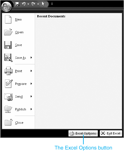
This section shows you how to display Excel options and provides an overview of what you might find on each tab. Later sections of this chapter cover each tab in detail. The entry to the Excel Options dialog is at the bottom of the Office icon menu, near the Exit Excel button, as shown in Figure 6.1.
Figure 6.1. The Excel Options button is on the Office icon menu.
Instead of tabs, the Excel Options dialog uses nine categories of options along the left side, as shown in Figure 6.2. When you choose a category on the left, the settings for that category appear on the right.
Figure 6.2. The Excel Options dialog has nine categories along the left side.
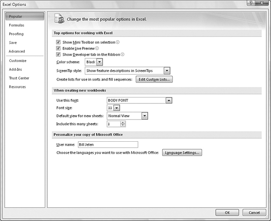
Table 6.1 shows the general types of settings you find in each category.
Table 6.1. Excel Options Dialog Box Settings
Getting Help with a Setting
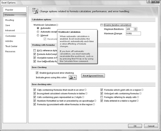
Many settings appear with a small i icon. If you hover the mouse near this icon, Excel displays a super ToolTip for the setting. The ToolTip explains what happens when you choose the setting and also provides some tips about what you need to be aware of when you turn on the setting. For example, the ToolTip in Figure 6.3 shows information about the calculation settings and also explains that you should use the F9 key to invoke a manual calculation.
Figure 6.3. You can see help on any setting by hovering over the i icon.
Toggling the New Excel 2007 Features
Some of the features in Excel 2007 are memory intensive. If your computer is running sluggishly, you can turn off several of these memory-intensive features, which are found in the Popular category of the Excel Options dialog:
- Show Mini Toolbar on Selection—This feature is popular in Word, but it rarely appears in Excel. You actually have to select a few characters from a cell while the cell is in Edit mode. The mini toolbar provides quick access to text formatting tools.
- Enable Live Preview—When you hover over a gallery, the worksheet previews the change before you click the gallery item.
You can also turn off the following features, which are found in the Advanced category:
- Alert the User When a Potentially Time-Consuming Operation Occurs—When this option is set, Excel alerts you when a potentially time-consuming operation occurs. By default, Excel warns you when an operation will affect more than 35,554 cells. You can change the cell threshold, or simply turn this feature off. If you are about to do a subtotals command, you need to invoke the command whether it will take a long time or not.
- Enable Multithreaded Calculations—This option enables multithreaded calculation, which affects you only if your computer has multiple processors (commonly referred to as “dual core”). Excel can now make use of both processors in order to speed up calculation time. Note that the first recalculation of any workbook takes longer than normal because Excel has to build two calculation trees. Subsequent calculations are faster.
- Group Dates in the AutoFilter Menu—This setting causes daily dates to be grouped into months and years for easy selection in the AutoFilter drop-down. Autofilters are discussed in Chapter 13, “Removing Duplicates and Filtering.”
Controlling the Look and Feel of the Worksheet Window
You might want to build a workbook that looks less like Excel because some people are intimidated by Excel. If you are building a workbook that must be distributed to many people who don’t regularly use Excel, having it look less like Excel can improve acceptance of the workbook.
The Excel Options dialog allows you to turn off many screen elements. In the Advanced category, in the Display section, you can turn off the formula bar. This is an applicationwide setting; that is, when you disable this setting, the formula bar is disabled in all workbooks.
The following settings affect the entire workbook:
- Show Horizontal Scroll Bar—You can uncheck this option to hide the scroll bar at the bottom of the screen.
- Show Vertical Scroll Bar—You can uncheck this option to hide the scrollbar at the side of the screen.
- Show Sheet Tabs—You can uncheck this option to prevent someone from seeing all the tabs. You would usually provide a menu sheet with hyperlinks to allow the person to change from sheet to sheet. Note that if someone knows the Ctrl+Page Down and Ctrl+Page Up shortcuts, that person will still be able to navigate to other worksheets in your workbook.
The following items apply only to the current worksheet:
- Show Row and Column Headers—This turns off the A, B, C, and so on column headers and the 1, 2, 3, and so on row numbers.
- Show Gridlines—This turns off the lines between cells.
![]()
To make the window look even less like Excel, you can hide the Ribbon by pressing Ctrl+F1 or remove the ribbon completely, as described in Chapter 38, “A Tour of the Best Add-ins for Excel.”
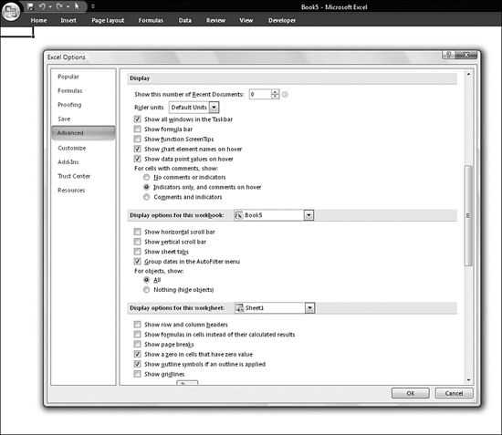
Figure 6.4 shows the Display settings in the Excel Options dialog. Behind the dialog box, you can see the Excel window with all elements removed.
Figure 6.4. You can make Excel look less like Excel by using these options.
Increasing Files in the Recent Documents List
The Office icon menu includes a list of your recently opened files. In previous versions of Excel, the default was to show four files in the list, and it could be increased to up to nine. In Excel 2007, the default is to show nine items in the list, and it can be increased to up to 50. If you increase this setting to 50 files, you can open any of the 50 recently used files simply by selecting it from the list.
To change the setting, you select the Office icon and then choose Excel Options, Advanced. In the Display section, you change Number of Documents in the Recent Documents List to the desired number of documents.
New in 2007: The Recent Documents list now includes files that you open directly from Windows Explorer. In previous versions of Excel, you had to use the Open or Save dialog to add a file to the recently used file list.
![]()
If you share a computer and are concerned about the files in this list, you can spin the option down to 0 and then click OK. This will completely remove the 50 files from the list.
If you routinely open more than 50 documents, yet you have certain favorite documents, you can force those favorites to always be in the Recent Documents list. Here’s how you do it:
- If one of you favorite file is not currently in the list of recent documents, open the file.
- Open the Office icon menu.
- Locate the item in the Recent Documents section. Click the pushpin icon that appears to the right of the filename, as shown in Figure 6.5. The pushpin turns green to indicate that this item is pinned to the menu.
Figure 6.5. You can pin your favorite files to the Recent Documents list.
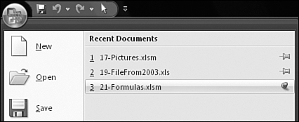
Any item with a pushpin will always appear in the Recent Documents list. Unfortunately, the pinned items do not always appear at the top of the list. The top spots are given to the files that you have had open most recently. If you pin several files to the list and then never open them again, those files will eventually move to the last spots on the list. However, because they are pinned, they will never fall off the end of the list.
To unpin an item from the Recent Documents list, you click the pushpin icon again.
Changing Gridline Color
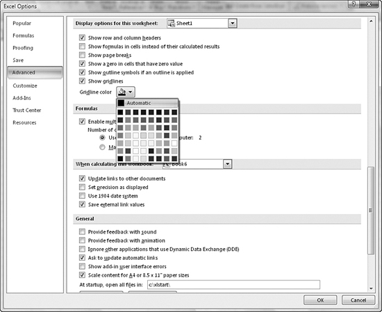
In previous versions of Excel, you had two choices for gridline color: gray and invisible. In Excel 2007, you can make the gridlines any of 56 colors. (It is not clear why Microsoft went back to a 56-color limit instead of 32-bit color scheme for this feature.)
To change the gridline color, you need to open the Excel Options dialog. Then you choose the Advanced category. Next, you scroll down to the Display Options for This Worksheet section. In the Gridline Color drop-down, you choose a color for the gridlines, as shown in Figure 6.6.
Figure 6.6. You can change the gridline color for the current worksheet.
Easing Entry of Numeric Data
A few options make it easier to enter a large range of numeric data. These functions are designed for people using the numeric keypad—which has the 10 digits, the four common operators, a decimal, and the Enter key—to enter numerals.
When you type a number in a cell and press the Enter key, Excel generally moves the cell pointer down one cell. This is fine if you are entering a column of numbers. However, if you would like to enter data in a row-by-row fashion, the default of moving the cell pointer down one row is frustrating.
You can specify that the cell pointer should move right, left, down, or up after pressing the Enter key. To do this, you choose the Office icon menu and then select Excel Options. In the Advanced section, you choose Editing Options. Then you change the setting for After Pressing Enter, Move Selection Direction, change the selection to Right. Note that if you uncheck the After Pressing Enter item, Excel keeps the cell pointer in the current cell when you press Enter.
Immediately below the After Pressing Enter setting, there is an option for automatically inserting a decimal point, assuming n decimal places. If you need to enter a range of figures in dollars and cents, you can use this setting to prevent you from having to type the decimal point. If you enter 123, Excel converts it to 1.23.
Guide to Excel Options
Table 6.2 shows every Excel feature that you can change in the Excel Options dialog. The table shows the feature, the category where it can be modified, the section within the category, and the text of the option.
Table 6.2. Excel Options, by Feature