
Chapter 29. Using Super Formulas in Excel
In this chapter
Using 3D Formulas to Spear Through Many Worksheets 824
Combining Multiple Formulas into One Formula 828
Calculating a Cell Reference in the Formula by Using the INDIRECT Function 830
Assigning a Formula to a Name 833
Replacing Multiple Formulas with One CSE Formula 838
Excel offers an amazing variety of formulas. This chapter covers some of the unorthodox formulas that you can build in Excel. In this chapter, you will learn about the following:
- Using a formula to add the same cell across many sheets
- Using a formula to reference the previous sheet
- Editing multiple formulas into one
- Assigning a formula to a name
- Letting data determine the cell reference to use with the
INDIRECTfunction - Using a dynamic range with an offset
- Transposing relative column references to rows
- Using
Row()orColumn()to return an array of numbers - Replacing thousands of formulas with one Ctrl+Shift+Enter (CSE) formula
- Using one formula to return a whole range of answers
- Doing conditional sums based on two or more conditions
Using 3D Formulas to Spear Through Many Worksheets
It is common to have a workbook composed of identical worksheets for each month or quarter of the year. Every worksheet needs to have the same arrangement of rows.
If you want to total a particular cell across all of the worksheets, you might try to write a formula with one term for each sheet; for example, =Sheet1!A1+Sheet2!A1+Sheet3!A1.... However, Excel supports a special type of formula that will spear through several worksheets to add a particular cell from each worksheet. The syntax of the formula is =SUM(Sheet1:Sheetn!A1).
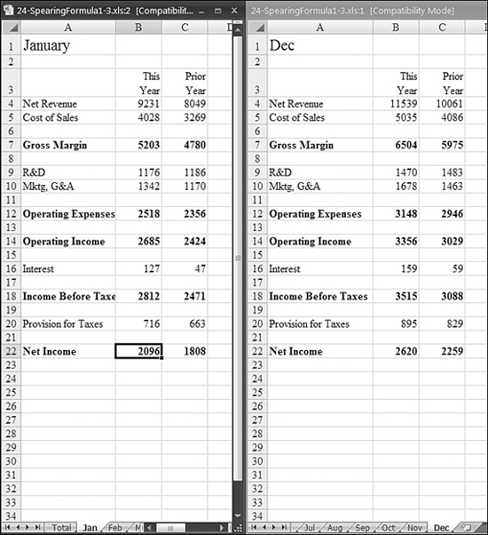
As shown in Figure 29.1, Net Income is in Row 22 on the January worksheet and is in the same row on the December worksheet. You cannot see this in Figure 29.1, but the arrangement of rows is identical on every worksheet.
Figure 29.1. The 12 workbooks, Jan through Dec, contain an identical arrangement of rows and columns.
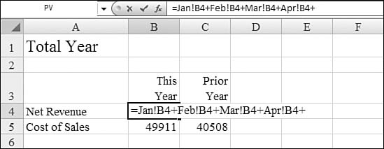
When creating a worksheet, you might be tempted to write a formula like the one in Figure 29.2 that adds up each of the 12 worksheets, but doing so would be rather tedious.
Figure 29.2. Writing a formula to point to all 12 worksheets would be tedious.
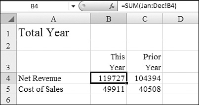
Instead, you can write a formula that totals Cell B4 from each worksheet, Jan through Dec. The syntax of the formula is =SUM(Jan:Dec!B4). After you enter this formula in Cell B4, you can easily copy it to all the other relevant cells in the worksheet, as shown in Figure 29.3.
Figure 29.3. This formula spears through 12 worksheets to total Cell B4 from each worksheet from Jan through Dec.
Referring to the Previous Worksheet
When you have an arrangement of several sequential worksheets, you might wish to keep a running total. This total would be calculated as the total on this sheet plus the running total from the previous sheet.
It is somewhat difficult to build a formula that will always point to the previous sheet. Many try this wrong approach: build a formula on Sheet2 that points to Sheet1. When you make copies of Sheet2, to Sheet3, Sheet4, and so on, the formula continues to always point back to Sheet1. This is rarely what you want.
The solution involves a tiny user-defined function that can be written in Excel’s macro editor.
This specific example shows you how to build a general purpose function that will return a value from a previous worksheet. This function can work in any situation.
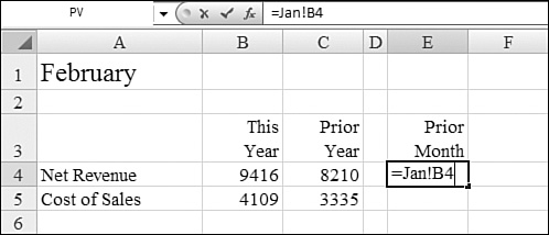
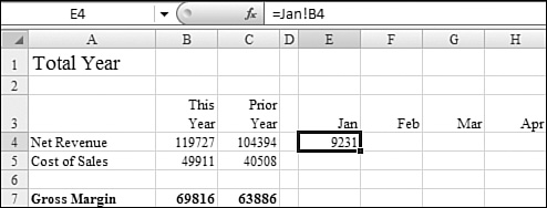
Figure 29.4 shows a formula that returns the value from the previous month. On the Feb worksheet, this would refer to =Jan!B4. You could easily copy this formula to other cells within the Feb worksheet. However, if you copy the formula to Mar or Apr, the formula still points to the Jan worksheet, which is not what you want.
Figure 29.4. You need to rewrite this formula for each of the 11 other months.
Excel offers a very cool solution to this problem. The solution requires a few lines of VBA macro code. Don’t be afraid. I will get you there and back without any problems. Here’s what you do:
- Press Alt+F11 to launch the VBA editor.
- In the VBA editor, choose Insert, Module.
- Type these lines in the blank module:
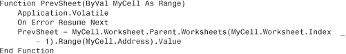
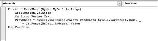
Your screen should look similar to Figure 29.5.
Figure 29.5. The VBA editor screen should look like this.
- Choose File, Close to return to Excel.
To realize the power of this function, you can put the workbook in Group mode and enter the function in 11 worksheets at once:
- Select the Feb worksheet.
- Hold down the Shift key while clicking on the Dec worksheet tab. This highlights all 11 worksheets. Although you are seeing the Feb worksheet, anything you do will also happen to all 11 selected worksheets.
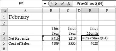
- In Cell E4, enter
=PrevSheet(B4), as shown in Figure 29.6.Figure 29.6. Although you see the Feb worksheet, this formula is also entered on all 10 other sheets in the group.
- Press Enter to accept the formula. The Feb worksheet picks up the value from Jan, but each additional worksheet picks up the value from the previous sheet, as shown in Figure 29.7.
Figure 29.7. One formula using the custom function
PrevSheetsolves the prior month problem seamlessly across all the worksheets.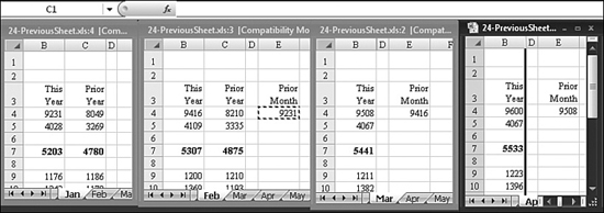
Tip From

To examine worksheets from the same workbook, select View, Window, New Window to create a second window of the workbook. Then select View, Window, Arrange, Vertical, OK to arrange the windows vertically. You now have two views of the same workbook, and you can change the right pane to be a different worksheet. The screenshot in Figure 29.7 reflects four new window commands before the windows are arranged vertically.
- With the worksheets still in Group mode, copy Cell B4 from the Feb worksheet to Cells B5, B7, and so on.
- Right-click any sheet tab and choose ungroup.
Combining Multiple Formulas into One Formula
With more than 350 functions available in Excel, it is possible to perform just about any calculation. Many times, however, it is easier to break the task down into many subformulas as you are trying to solve the problem.
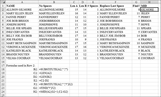
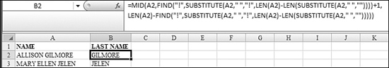
For example, fellow Excel MVP and guru Bob Umlas once taught me that I could use the Substitute function to locate the last space in a word. This is handy for finding the last word in a sentence or name. However, unlike Bob, I always need to build this formula over the course of several columns. It takes me seven columns to do a trick that Bob can do in one. Figure 29.8 shows all the formulas used to replicate the trick.
Figure 29.8. It takes me seven formulas to isolate the last name.
After you have puzzled out a complicated set of interrelated functions to achieve a result, you can begin consolidating the formulas into one monster formula.
There is an easier way to combine many formulas into one formula. In general, follow these steps:
- Examine the final formula. It will reference cells that contain one or more subformulas. Let’s say that one of the subformulas is a cell such as ZZ123.
- Move the cell pointer to the subformula in ZZ123.
- Press F2 to put the formula in edit mode.
- With the mouse, highlight the formula in the formula bar, but do not highlight the equals sign in the subformula.
- Press Ctrl+C to copy this portion of the subformula to the clipboard.
- Go back to the final formula. Press F2 to put the formula in edit mode.
- In the formula bar, using the mouse, highlight the characters that point to the subformula. In this case, it is cell ZZ123.
- Press Ctrl+V to paste the subformula in place of the ZZ123 reference.
- Press Enter to accept this intermediate formula.
- If there are additional references to a cell with a subformula in the final formula, repeat steps 1-10 for the next reference.
I realize this may be difficult to follow in the abstract. If you would like to follow along with a real example, follow these steps:
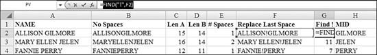
- In Cell H2, the formula has a reference to Cell G2, as shown in Figure 29.9.
Figure 29.9. The goal is to replace G2 in this formula.

- Move the cell pointer to G2.
- In the formula bar, click and drag with the mouse to select all the characters in this formula except the equals sign, as shown in Figure 29.10.
Figure 29.10. Copying characters from the formula bar is different from copying a cell.
- Press Ctrl+C to copy the selected characters to the Clipboard.
- Press Esc to exit Edit mode.
- Move the cell pointer back to Cell H2 and highlight the characters
G2in the formula bar, as shown in Figure 29.11.Figure 29.11. With the formula from Cell G2 on the clipboard, you select G2 in the final formula.
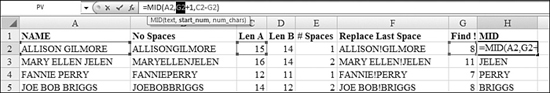
- Press Ctrl+V to replace
G2with the formula from Cell G2, as shown in Figure 29.12Figure 29.12. You can press Ctrl+V to paste the characters from the Cell G2 formula instead of the reference to Cell G2.
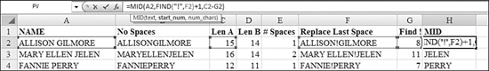
- Repeat this process to replace the other
G2andC2in the Cell H2 formula. Note that pasting the formula from Cell G2 introduces references to Cell F2. - Continue to replace any reference to a column other than Column A. After doing several copy and paste operations in the formula bar, you eventually end up with one monster formula.
- Delete Columns B through G. People will be impressed with how you were able to write such an amazing formula (see Figure 29.13). In fact, someone might even say to you, “Wow! You are as smart as Bob Umlas!”
Figure 29.13. After several iterations of replacing references in the formula, you end up with one monster formula to replace the six subformulas.
Calculating a Cell Reference in the Formula by Using the INDIRECT Function
Usually a formula points to a particular cell or range of cells. Sometimes, though, you want a formula to point to a different cell as the result of a calculation. You can do this by using the INDIRECT function.
In general, this process involves writing a text-based formula that evaluates to a cell address. Although your particular situation will certainly be different, here are some examples of formulas that evaluate to a cell address:
- =CHAR(64+COLUMN(B275)&ROW(ZZ999)—evaluates to B999.
- =“Sheet”&ROW(A1)&"!C2”—evaluates to Sheet1!C2 in the current row, but to Sheet2!C2 when copied down one row, and to Sheet3!C2 when copied down to a third row.
- =CHAR(65+MONTH(A1))&“19”—evaluates to row B19 in January, C19 in February, and so on.
After you have a formula that evaluates to text that looks like a cell reference, you can use that formula as the argument to the INDIRECT() function. Excel will return the value in the cell indicated by the text formula.
One concrete example: if cell Z99 contains the value 1, then the formula of =INDIRECT("Z99") will return a value of 1. A more practical concrete example follows.
Say that in Figure 29.14, you would like to build a table to copy the current-month totals from each worksheet to a summary table on the Total worksheet. Without the INDIRECT function, you would have to separately enter 12 different formulas in Row 4—one for each month (for example, =Jan!$B4 for January, =Feb!$B4 for February, and so on).
Figure 29.14. The first of 12 different formulas required in E4:P4.
You can solve this problem with a single formula that you can copy to the entire total worksheet. Follow these steps:
- You will want to design a text formula in Cell E4 to point to the correct sheet and cell.
- The worksheet has month headings in Row 3, so you can start to build a formula as
=E$3&"!". Note that the$before the3ensures that as the formula is copied to lower rows in the summary table; it will always point to the month heading in Row 3. - The next trick is finding a function that will return the address of Column B for Row 3. To do this, you can use the versatile function called
CELL. TheCELLfunction can return many bits of information about a reference, including the address of the cell. For example,=CELL("address",$B4)returns the text$B$4. - Figure 29.15 shows the intermediate result of entering
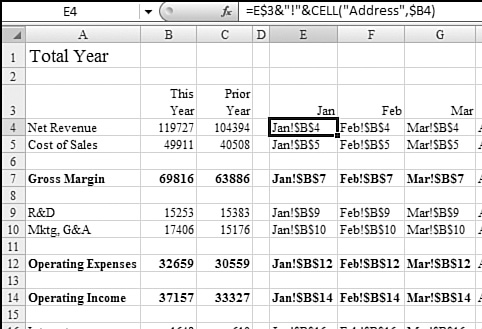
=E$3&"!"&CELL("Address",$B4)into the table.
Figure 29.15. All the formulas in E4:P22 are identical, but they return the reference to the cell from which the result should be copied.
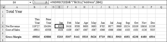
The last step is to wrap the INDIRECT function around the formula in Cell E4. This tells Excel to evaluate the function inside INDIRECT to learn that Excel should return the value from Cell B4 on the Jan worksheet.
The whole trick to being efficient in Excel is being able to write one formula that can be copied to an entire range. Rather than going through the tedium of entering 12 different formulas in Row 4, you can use the INDIRECT function to enter just one formula everywhere in the range (see Figure 29.16).
Figure 29.16. You can wrap the formulas in the INDIRECT function to allow one formula to fill the entire table.
Note
Excel gurus will point out another benefit of the INDIRECT function. If you have a formula such as =SUM(A1:A10), and you insert a new Row 5, the formula normally expands to =SUM(A1:A11). However, there might be a time when you really want to sum only the first 10 records on the sheet. In this case, you can use the formula =SUM(INDIRECT("A1:A10")) to always point to Rows 1 through 10, no matter what rows are inserted or deleted.
Caution
There is an important limitation with INDIRECT functions. If you build an INDIRECT function that points to an external workbook, the formula works only when the external workbook is open.
Using Offset to Refer to a Range That Dynamically Resizes
When you first read the Help topic on the OFFSET function, you might wonder what would be the point of such a function. The OFFSET function allows you to describe a range by specifying five parameters:
- Any cell from which to start.
- The number of rows to move from the original cell in order to get to the upper-left corner of the reference. Positive numbers move down the worksheet, and negative number move up the spreadsheet.
- The number of columns to move from the original cell in order to get to the upper-left corner of the reference. Positive numbers move to the right from the original cell, and negative numbers move to the left.
- The number of rows in the reference.
- The number of columns in the reference.
It would be difficult to imagine why you would ever use =OFFSET(A1,2,3,4,5) to refer to the range D3:H6. However, when you consider that these arguments can be functions that calculate the size of a range, it starts to make sense.
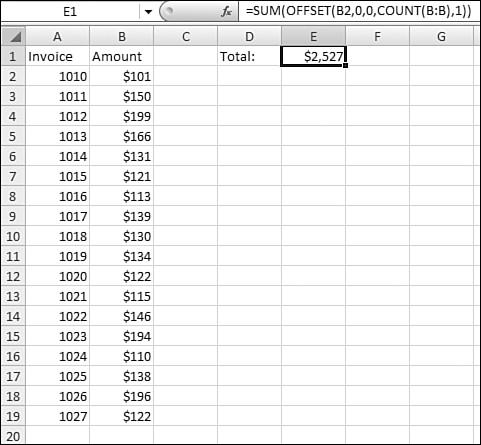
Say that you start entering invoice amounts in Cell B2 and proceed down Column B. In order to write a sum formula that can expand to include any number of entries in Column B, you could count the number of numeric entries in Column B by using =COUNT(B:B). If you then use the COUNT function as the fourth argument in the OFFSET function, you have set up a dynamic formula that will always expand as new items are entered, as shown in Figure 29.17.
Figure 29.17. The OFFSET function allows you to describe a rectangular range that starts a calculated number of rows and columns from a starting point.
Assigning a Formula to a Name
When you set up a named range, the Names box shows that the name has a value like =Sheet1!A1. Because this value contains an equals sign, you know that this value is actually a formula.
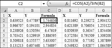
It is possible to assign a very complex formula to a name. Say that you have a workbook with 100 worksheets, with 20 columns of X and Y data in each worksheet, as shown in Figure 29.18. You want to continually update a transformation formula used on all the X and Y points. Every time the formula changes, you have to copy the new formula to all 20 columns on the 20 worksheets.
Figure 29.18. Every time the formula changes, you must copy it to 400 non-adjacent columns.
The technique involves writing a relative formula that will carry out the same transformation as your original formula. Assign this formula to a name. In each of the cells, use =NamedFormula instead of the formula.
The advantage is that you can now edit the formula in the Edit Name box and the new formula will be used throughout the workbook.
The following specific examples walk through the steps for one particular formula.
While you usually write formulas in A1 notation made popular by VisiCalc and Lotus 1-2-3, Microsoft still supports the old R1C1 notation that was used in Microsoft Multimate back in 1982. In the R1C1 notation, a cell such as E2 is referenced as R2C5, meaning Row 2, Column 5. The following tip makes use of R1C1 notation.
You can use an R1C1 version of the INDIRECT function to create a formula to take the cosine of a cell two cells to the left of the formula cell and divide it by the sine of the cell to the left of the formula cell. To do so, you follow these steps:
→ For a complete discussion of R1C1 style references, see “Using R1C1 Style Formulas,” page 987, in Chapter 36.
- To take the cosine of a cell two cells to the left of the current cell, use
=COS(SUM(INDIRECT("RC[-2]",False))). - To take the sin of the cell to the left of the formula cell, use
=SIN(SUM(INDIRECT("RC[-1]",False))). - Use Formulas, Named Cells, Name Manager to open the Name Manager dialog box.
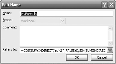
- Use the Name Manager dialog to assign the formula
=COS(SUM(INDIRECT("rc[-2]",FALSE)))/SIN(SUM(INDIRECT("rc[-1]",FALSE)))to a name such as MyFormula, as shown in Figure 29.19.Figure 29.19. You can assign a name to a formula.
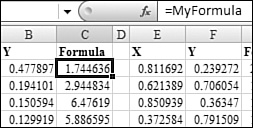
- In each worksheet, replace the current formula with
=MyFormula, as shown in Figure 29.20.Figure 29.20. One last time, you copy the formula name to all 400 non-adjacent columns.
- Change the formula in the Edit Name dialog box and have the new calculation carried out in all 400 non-adjacent columns.
Turning a Range of Formulas on Its Side
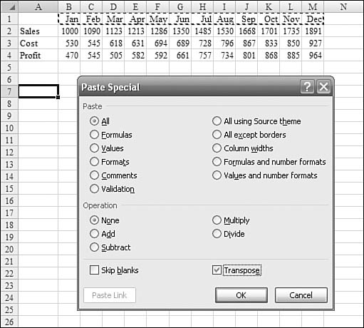
The Transpose option in the Paste Special dialog is great for changing values that span across several columns into values that go down a column. Here’s an example:
- In Figure 29.21, you select B1:M1 and then press Ctrl+C.
Figure 29.21. You can copy a range that spans several columns.
- Select the top left cell where the range should be copied. In this example, select cell A7.
- Select Home, Clipboard, Paste, Paste Special to open the Paste Special dialog.
- Select Transpose in the Paste Special dialog.
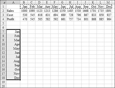
- Click OK. The month names now go down the row, as shown in Figure 29.22.
Figure 29.22. You can use the Paste Special dialog to turn a range on its side.
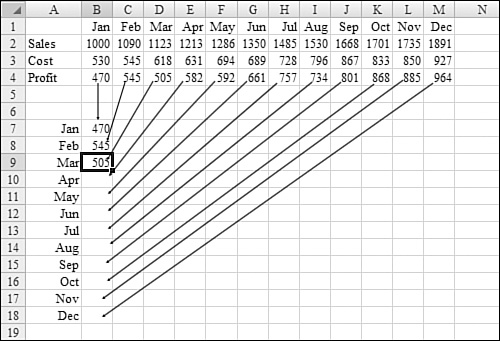
However, there is not a good way to copy the calculation for profit from Row 4 to the new table. You normally have to enter 12 different formulas in the range B7:B17 as shown in Figure 29.23.
Figure 29.23. Transposing with a formula requires a different formula in each cell.
But there are two ways to easily enter a single formula that will turn those results on their side.
First, you can use the OFFSET function you learned about earlier in this chapter. You can set up an OFFSET function that points to $A$4 and offsets by an additional column as you copy the formula down the rows. Try it:
- In Cell B7, enter
=ROW(A1). The result is the number 1. - Copy the formula from Cell B7 down to B7:B18. The result returns a string of integers from 1 through 12, as shown in Figure 29.24
Figure 29.24. You can copy the
=ROW(A1)formula down a column to create a sequence of integers.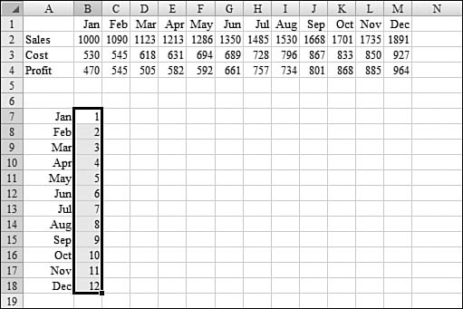
- Use the formula
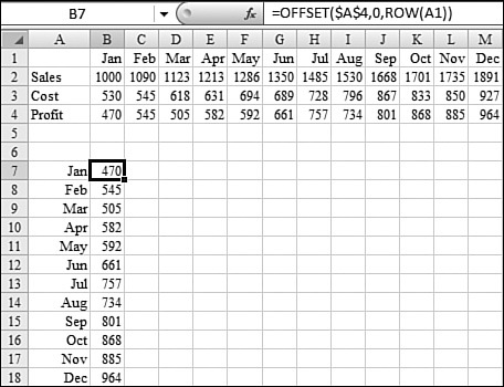
=ROW(A1)as the third argument in theOFFSETfunction. A formula of=OFFSET($A$4,0,ROW(A1))will achieve the perfect result, as shown in Figure 29.25.
Figure 29.25. You can use the ROW(A1) trick as the Column Offset parameter in the OFFSET function to turn a range on its side.
One danger exists with just about every method described in this chapter: They produce results that the average person does not understand. So if you want to end up with straightforward formulas in B7:B18, you can use the following method:
- Enter a formula such as
=B4in Cell B5. - Copy the first formula across Row 5 for each month.
- Highlight the formulas in B5:M5.
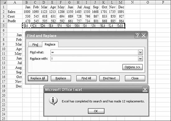
- Use Home, Editing, Find & Select, Replace to display the Find and Replace dialog. In the Find What box, enter an equals sign. In the Replace With box, enter an exclamation point. Click Replace All to change every occurrence of
=to!. This converts the formulas to text, as shown in Figure 29.26.Figure 29.26. Converting the formulas to text allows them to be transposed.
- Copy the range and highlight a new cell (in this example, Cell B7).
- Choose Home, Clipboard, Paste, Paste Special to open the Paste Special dialog and then select Transpose. Because the cells are all text, they transpose perfectly, as shown in Figure 29.27.
Figure 29.27. You change
!back to=to change to formulas.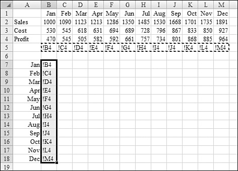
- Use Home, Editing, Find & Select, Replace to display the Find and Replace dialog. Type an exclamation point in Find What and an equals sign in Replace With. Click Replace All to change every
!back to=. It now looks as if you actually typed all 12 formulas individually.
Replacing Multiple Formulas with One Array Formula
There exists a wildly powerful type of formula that most Excel users have never experienced. This formula can do thousands of calculations in a single formula.
The formula is known as an array formula. You must use Ctrl+Shift+Enter when entering an array formula to tell Excel to evaluate the formula as an array.
Here is an example of the power of an array formula.
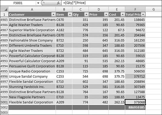
Consider the dataset shown in Figure 29.28. This database has transactional data showing quantity, unit price, and unit cost. The goal is to enter a single formula that will multiply each quantity by each price and sum the result.
Figure 29.28. The goal is to find the result of multiplying quantity by price for all records.
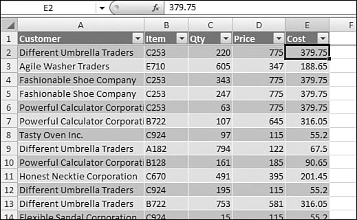
Most people would add a new column with formulas to multiply quantity times price as shown in Figure 29.29. This is easy to do. However, it adds 5,000 new formula cells to your worksheet.
Figure 29.29. The typical approach to summing 5,000 calculations is to add a new column with the calculations and total that column.
It is possible to enter a calculation in one cell that will do the 5,000 calculations and total them. With tables in Excel 2007, you have two choices for writing this formula:
- =SUM(C2:C5000*D2:D5000) is an example of a formula for a range that has not been converted to a table.
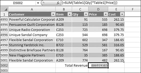
- =SUM(Table1[Qty]*Table1[Price]) is an example of a formula for a range that has been converted to a table
Follow these steps:
- Select a blank cell in the worksheet.
- Type either formula previously shown.
- Hold down Ctrl+Shift+Enter.
As shown in Figure 29.30, Excel will correctly calculate the result.
Figure 29.30. When you press Ctrl+Shift+Enter, Excel understands that this is not a typical formula.
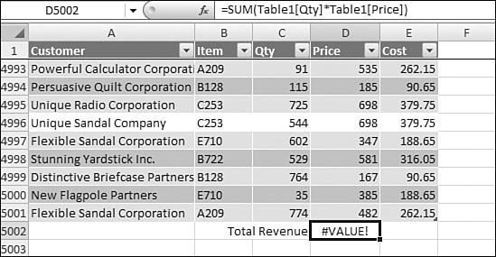
If you fail to use Ctrl+Shift+Enter, Excel will return a #VALUE error, as shown in Figure 29.31.
Figure 29.31. If you don’t press Ctrl+Shift+Enter, the formula returns a #VALUE! error.
Excel in Practice: Copying Array Formulas
There is a difficulty when copying array formulas. In Figure 29.32, the array formula in B5006 needs to be copied to B5006:K5025.
Figure 29.32. You want to copy this formula to the rest of the summary table.
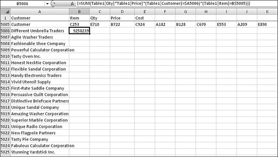
Normally, you would copy Cell B5006 and then paste to Cells B5006:K5025. With array formulas, this leads to an error. If you attempt to do this copy, you are told that you cannot move or change part of an array. The solution is to do the copy in two pieces:
- Copy Cell B5006 to B5007:B5025.
- Copy B5006:B5025 and paste it to C5006:K5006.
Finding Conditional Sums by Using SUMPRODUCT
It is possible to convert the previous array formula to a SUMPRODUCT formula:
![]()
You can then enter this as a regular formula instead of an array.