Chapter 31. Using What If, Scenario Manager, Goal Seek, and Solver
In this chapter
When Dan Bricklin invented VisiCalc in 1979, he was trying to come up with a tool that would let him recalculate his MBA school case studies quickly. Almost three decades later, spreadsheets are still used for the same functionality.
Newer spreadsheet tools such as Goal Seek and Solver allow you to back directly into the assumptions that lead to a solution. This chapter discusses some of Excel 2007’s feaures that are helpful when you are tying to find a specific answer.
Using What-If
Once you have set up a model in Excel, it is very easy to make copies of the model side by side and then change the various input variables to test their impact on the final result. Because this type of analysis answers the question of what happens if a change is made, it is known generically as what-if changes.
What-if analyses are the least formal method in this chapter. You simply copy the input variables and formulas multiple times. You can then vary the input variables until you reach a suitable solution.
For example, Figure 31.1 shows a worksheet to calculate the monthly payment on a new car purchase. In Cells E1, E2, and E3 are the known values: the price, term, and interest rate. Cell E4 calculates the monthly payment, using the =PMT() function.
Figure 31.1. You may not like the answer in Cell E4, but Excel makes the answer easy to find.
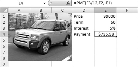
Cells E1:E4 are a self-contained mini-model. You can easily copy these cells several times over and perform what-if analysis on the car payment model.
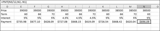
Figure 31.2 shows a basic what-if worksheet. You can use this worksheet to manually plug in different numbers. Columns F and G show the effects of changing the number of months. Columns H:J factor in a lower interest rate. Columns K:M show the effects of finding a lower price. Based on a number of options, Column N starts to hone in on a scenario to get to the $695 target payment: Use 63 months, 5% interest, and a price of $38,500.
Figure 31.2. By making multiple copies of the table, you can create a simple What-If model.
There is nothing magic about what-if analyses. There are no ribbon commands involved. You simply copy the model and plug in a few different numbers. The remaining topics in this chapter are more structured with better features.
Creating a Two-Variable What-If Table
The analysis in Figure 31.2 is fairly ad hoc. It basically enables you to try various combinations until you find one that is close to your target payment. If you have two variables to manipulate, you can use Excel’s fairly powerful Data Table command. To use a data table, follow these steps:
- Enter a formula in the upper-left corner of the table. This formula should point to at least two variable cells.
- Along the left column of the table, enter various values for one of the input values.
- Along the top row of the table, enter various values for the other input variable.
- Select the entire table.
- From the Data ribbon, select Data Tools, What-If Analysis, Data Table.
- In the Data Table dialog box, enter a row input cell and a column input cell.
- Click OK to complete the table.
For example, you can use the Data Table command to try to negotiate on price and term of the loan by following these steps:
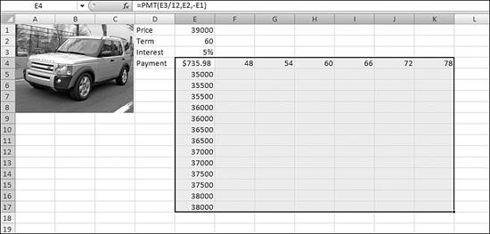
- Use the formula in Cell E4 as the formula in the top-left corner of your table.
- From E5:E17, fill in various possible values for purchase price.
- From F5:K5, fill in various possible values for the term of the loan.
- Select the entire table, E4:K17, as shown in Figure 31.3.
Figure 31.3. Preparing for a two-variable what-if analysis.
- Select Data Table from the Data ribbon to display the Data Table dialog box, as shown in Figure 31.4. The dialog box asks you for a row input cell and a column input cell. The Row Input Cell field offers to take each value from the top row of the table and plug it into a particular cell.
Figure 31.4. Setting up the Table dialog.
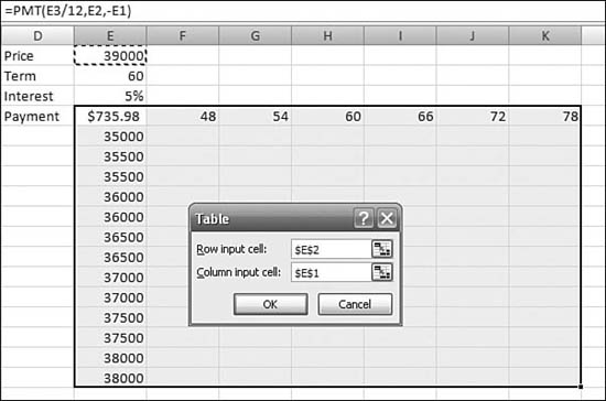
- Because the values in F5:K5 are loan terms, specify E2 for the row input cell.
- Similarly, the Column Input Field offers to take each value from the left column and replace that value in a particular cell. Because these cells contain vehicle prices, choose E1 as the column input cell.
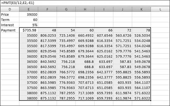
- Click OK. Excel fills in the intersection of each row and column with the monthly payment, based on the price in the left column combined with the loan term in the top row. Figure 31.5 shows the resulting table.
Figure 31.5. Excel performs 78 what-if analyses in one command.
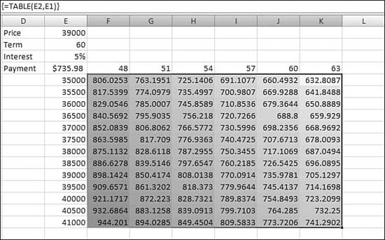
- Reselect just the interior of the table. You can see that Excel represents the table with the
TABLE()array function. Figure 31.6 shows the table with a heat map applied.
Figure 31.6. The values in the table are calculated by a single TABLE() array formula.
→ For more information on data visualizations, see “Creating Heat Maps with Color Scales,” page 158 in Chapter 9.
Note
Note that the values calculated in the table are live formula values. If you change the numbers along the edge of the table, the TABLE() array formula recalculates new loan payment amounts.
Using Scenario Manager
The Data Table command is great for models with two variables that can change. Sometimes, however, you have models with far more variables that can change. In such a case, you should use the Scenario Manager, which allows you to create multiple scenarios, each changing up to 32 variables.
With up to 32 variables changing, it is best to use named ranges for all the input variables before you define your first scenario. One of the results of the Scenario Manager is a summary report. Using named ranges for all the input cells makes the report far easier to understand.
→ To learn how to use named ranges to your advantage, see “Using Named Ranges to Simplify Formulas,” page 846, in Chapter 30.
Generally, Scenario Manager allows you to set up named scenarios such as “Best Case,” “Worst Case,” and “Most likely.” In each scenario you can specify values for up to 32 variables.
You would then have a model that calculates results based on the 32 input variables. For example, you might have a business plan that projects sales for the next 120 months using growth rates in the input variable section of the spreadsheet. The important distinction is that while you may only have 32 input variables, you might base millions of formulas on these 32 input variables.
Use the Scenario Manager dialog box to quickly switch to a different set of input variables. The worksheet can quickly be calculated using Best Case and Worst Case scenarios.
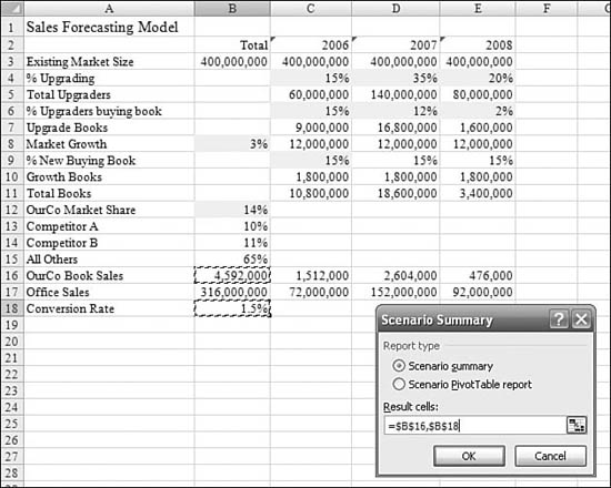
For a specific example, Figure 31.7 shows a sales forecasting model. All the highlighted cells are variables that can change. The model calculates a total forecast in Cell B16 and a ratio in Cell B18. To set up and use scenarios, follow these steps:
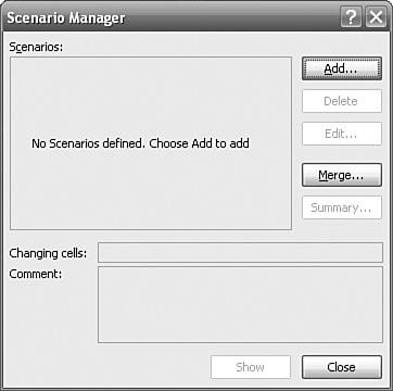
- Select Data, Data Tools, What-If Analysis, Scenario Manager to display the Scenario Manager dialog. Initially, the Scenario Manager indicates that there are no scenarios defined, as shown in Figure 31.8.
Figure 31.7. This forecast model is based on nine variable cells.
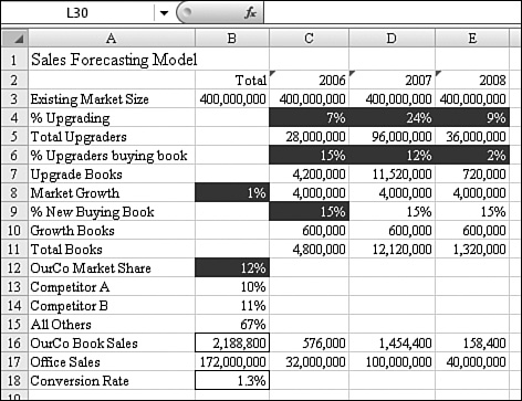
Figure 31.8. The Scenario Manager dialog before you add the first scenario.
- Click the Add button to add the first scenario. The Edit Scenario dialog appears.
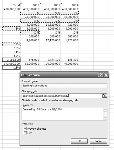
- In the Edit Scenario dialog, choose which cells will be changing. Because the variable cells are not adjacent, select the first contiguous range and then Ctrl+click to add additional ranges, as shown in Figure 31.9.
Figure 31.9. You Ctrl+click to select all the changing cells.
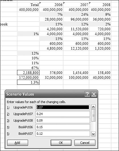
As shown in Figure 31.10, the Scenario Values dialog box appears, in which you can edit the values for each starting cell. It is a little annoying that this dialog can show only five values at a time. If your model contains the maximum of 32 values that can change, you have to scroll several times to see all the values in this dialog.
Figure 31.10. You use the Scenario Values dialog to edit values for a scenario.
- Edit any values in the Scenario Values dialog. If you have additional scenarios to add, click the Add button. When you are done assigning scenarios, click OK.
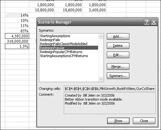
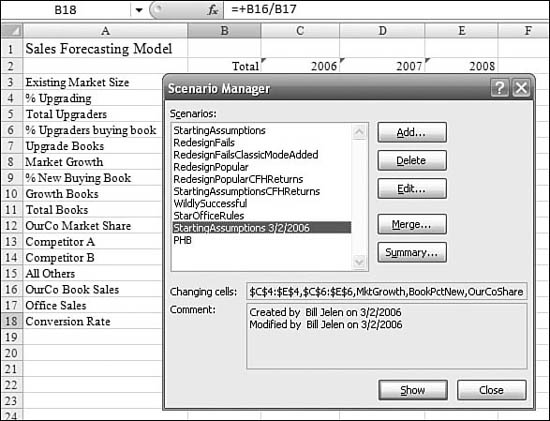
- Try switching between scenarios in the Scenario Manager by either double-clicking a scenario or clicking the scenario and clicking Show, as shown in Figure 31.11. If you are going to add a new scenario similar to one existing scenario, show that scenario before clicking Add.
Figure 31.11. The new scenario is shown behind the dialog box after you double-click a scenario name.
Creating a Scenario Summary Report
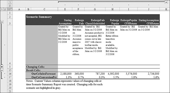
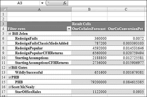
One powerful feature of Excel scenarios is the ability to create a scenario summary report. When you click the Summary button on the Scenario Manager dialog, Excel allows you to choose either a scenario summary report or a pivot table report. In either case, you should select one or more cells that represent the results of the model. For example, Figure 31.12 shows OurCo Book Sales and Conversion Rate selected.
Figure 31.12. You can hold down Ctrl to select more than one result cell.
After specifying the results cells, the scenario summary report is added on a new worksheet in the workbook. This is an amazingly useful report that has a number of useful features.
After the initial creation, the summary is as shown in Figure 31.13. Notice that there are group and outline buttons along both the rows and the columns of the report. The plus sign next to Cell A3 indicates that the comments in Row 4 are currently hidden.
Figure 31.13. The default scenario summary report.
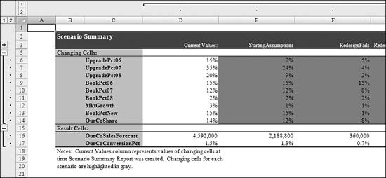
You can use word wrapping in a summary report. For example, Figure 31.13 shows that word wrapping was used to make the headings in Row 3 appear on two lines and that the column widths were adjusted. You will probably always have to make these adjustments to make your summary reports look better.
Figure 31.14. You can adjust word wrapping and column widths.
Tip From
![]()
To force word wrapping in the middle of a cell, you position your mouse cursor at the break point and press Alt+Enter.
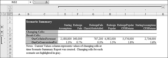
If you click the minus sign next to Row 5, you can hide the assumption cells and just show the results, as shown in Figure 31.15.
Figure 31.15. If your manager’s eyes glaze over with a table of numbers, you can show just the results.
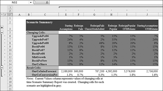
As you create each scenario, the Scenario Manager adds a comment with your name and the date and time. You can also add your own comments. As shown in Figure 31.16, you can click the plus sign next to Row 3 to reveal the comments in the report.
Figure 31.16. You can show comments in a report.
Caution
The scenario summary report is a snapshot in time. If you later change scenarios or add new scenarios, you have to re-create (and re-format) the scenario summary report.
Adding Multiple Scenarios
You might want to share a workbook with others and have them add their own scenarios so that you can get opinions from people in other areas of your company, such as sales, marketing, engineering, and manufacturing. To do this, follow these steps:
- Save the workbook with just the starting scenario.
- Route the workbook to each person. In a hidden field, Excel keeps track of who adds each scenario.
- When you get the routed workbook back, open both the original workbook and the routed workbook.
- Display the Scenario Manager in the original workbook.
- Click the Merge button in order to display the Merge Scenarios dialog, as shown in Figure 31.17.
Figure 31.17. Merging scenarios from a workbook routed to others.
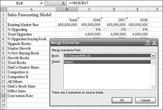
- In the Book drop-down, choose the name of the routed workbook. In Figure 31.17, the dialog shows that two scenarios are available on Sheet 1.
- Excel usually encounters identically named scenarios in the merge process. It differentiates any scenarios with identical names by adding a date or name to the incoming scenarios as shown in Figure 31.18. If these scenarios are truly identical to the scenario that you originally sent out, delete those scenarios.
Figure 31.18. Merged scenarios are added to the bottom of the list.
- In the Scenario Manager, click Summary. The Scenario Summary dialog appears.
- In the Scenario Summary dialog, click Scenario PivotTable report. The initial pivot table appears, as shown in Figure 31.19.
Figure 31.19. The default pivot table shows scenarios from all people on the routing list.
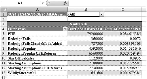
- Drag the field from the Report Filter area to be the first Row Labels field. You can now see scenarios grouped by author. As shown in Figure 31.20, although this is an interesting view, there is not a good way to see the assumptions that each author used to arrive at his or her results.
Figure 31.20. You can move the field from the Report Filter to the first row label in order to compare scenarios by person.
Using Goal Seek
Have you seen the television show The Price Is Right? One of the games on the show is the Hi Lo game. A contestant tries to guess the price of an item, and Bob Barker tells the player that the actual price is higher or lower. The process of honing in on a price of $1.67 might involve guesses of $2, $1, $1.50, $1.75, $1.63, $1.69, $1.66, $1.68, and $1.67. Using the techniques described so far in this chapter, you might find yourself playing this game with Excel to try to narrow in on an answer.
You might have an Excel worksheet set up that calculates a final value using several input variables. How can you solve the formula in reverse? You want to find input variables that will generate a certain answer.
One difficult option is to determine if there is another Excel function that reverses the calculation. For example, =ARCSIN() performs the opposite of =SIN().
Another difficult option is to use algebra to attempt to solve for one of the input variables.
Mostly, though, I find people will simply play the “Hi-Lo” game, successively plugging in higher and lower answers to the input cell until they narrow in to an input variable that produces the desired result.
If you’ve ever found yourself playing the Hi-Lo game, check out the Goal Seek command. This command will, in effect, play the Hi-Lo game at hyperspeed, arriving at an answer within a second.
Consider the car payment example at the beginning of the chapter. You want to find a price that yields a $695 monthly payment. If you do some research, you might find the =PV() function that can solve this. Most people will simply plug in successively higher or lower values for the price in Cell E1 (refer to Figure 31.21).
Figure 31.21. Goal Seek lets you find one value by changing one other cell.
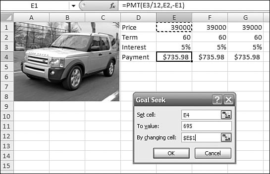
Excel has an option that allows you to quickly hone in on a value. It is called Goal Seek. To use Goal Seek, follow these steps:
- Select the answer cell. In this example, it would be the payment in Cell E4.
- From the Data Tools group of the Data ribbon, select the What If Analysis drop-down and then choose Goal Seek. The Goal Seek dialog appears, as shown in Figure 31.21.
- In the Goal Seek dialog, indicate that you want to set the answer cell to a particular value by changing a particular input cell. In this example, you want to set cell E4 to the value of $695 by changing Cell E1. Excel quickly tries to hone in on a value. When Excel gets to within a penny of the value, the Goal Seek Status dialog appears, as shown in Figure 31.22. This dialog reports that it was trying to reach a target value of $695 and was able to reach that value. Behind the dialog, the worksheet shows the proposed price of $36,828.54 in the worksheet.
Figure 31.22. You can choose to accept the proposed solution or revert to the previous numbers.
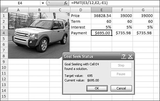
- Either accept this value by clicking OK or revert to the original value by clicking Cancel.
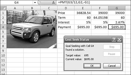
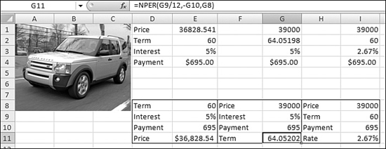
Goal Seek is great for quick calculations. Figure 31.23 shows an example in which two additional Goal Seek operations have been done. One operation set Cell F4 to $695 by changing the term in Cell F2. The next operation set Cell G4 to $695 by changing the interest rate in Cell G3.
Figure 31.23. Three different Goal Seek commands find how to yield a $695 payment by changing either the price, term, or rate.
Is It Cheating to Use Brute Force to Think Less?
Most of the time when you could use Goal Seek, there is a brainier solution. If you have a complex series of formulas set up using just the +, -, *, /, and ^ operators, you could almost certainly get out a pencil and do the algebra required to derive the formula you need.
In the preceding text, Figure 31.23 shows how you can use Goal Seek to figure out how to achieve a certain monthly payment by changing three different cells. Besides Goal Seek, Excel provides a function that can correctly find the term for a given price, interest, and payment: the NPER() function. For example, as shown in Figure 31.24, you can use the NPER() function in Cell G11 to calculate a more exact version than Goal Seek is able to discover. Similarly, in Cell E11 you can use =PV(E9/E12,E8,-E10) to discover the present value (that is, the vehicle price) of a loan. In Cell I11 you can use =RATE(I9,-I10,18)*12 to discover the rate needed to generate a monthly payment of $695 for a certain price and term.
Figure 31.24. Goal Seek prevents you from having to learn functions such as NPER().
Excel might have to go through 100 iterations of a lightning-fast Bob Barker–style Hi Lo game in order to find the solution, but it usually finds that solution within a second or two. This is definitely faster than using paper and pencil to do the algebra or pulling out this book to learn about the NPER() function. If you are a loan officer at a bank, it might be worthwhile for you to learn how to use the NPER() function. However, if you are using this worksheet once every four years to figure out your next car purchase, it is perfectly fine to let Excel sweat through the brute-force calculations with Goal Seek.
Troubleshooting Tip: When Goal Seek Won’t Work
Some problems are not well suited to using Goal Seek. Goal Seek needs a clear mathematical relationship between the starting and ending cells. For example, the model in Figure 31.25 is set up to choose from among 20 different package plans. Each package offers a different number of tickets, meals, and vouchers. Cell E1 chooses a particular plan, and Cell E2 uses the INDEX() function to calculate the number of tickets associated with the plan. Because there is no mathematical sequence to the number of tickets in each plan, Goal Seek will have little chance of succeeding in this situation.
Figure 31.25. Because there is no mathematical order to the number of tickets offered in each plan, Goal Seek has little chance of finding a solution in this case.
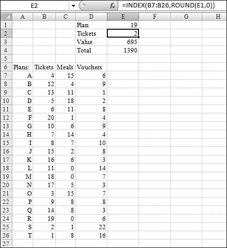
Say that you want to set the Total value in Cell E4 equal to 6950. A quick scan through the list of plans shows that Plan G offers 10 tickets, which would be worth exactly $6,950. However, Excel will have no chance of figuring this out using Goal Seek.
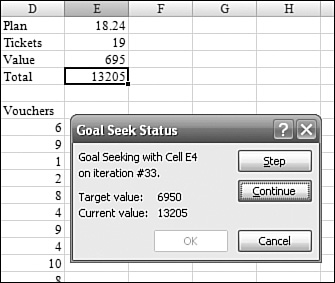
The following steps illustrate how you can watch the Goal Seek process in slow motion to see if Excel is getting closer:
- Start Goal Seek. An answer is not immediately found.
- Click the Pause button on the Goal Seek Status dialog. As shown in Figure 31.26, Excel is on its 33rd attempt at finding a value. In this pass, Excel is trying 18.24 in Cell E1. This is producing a value of 13205 instead of the desired value of 6950.
Figure 31.26. You can click Pause to examine how Excel is trying to solve the problem.
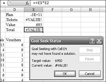
- Click the Step button to proceed to the next guess. On the 34th iteration, Excel tries a plan of 13500743, which produces a
#REF!error. Excel successively tries higher and higher values until, on step 64, it goes back to trying 18.24. Eventually, after 100 iterations, Excel gives up and reports that it cannot find a solution, as shown in Figure 31.27.
Figure 31.27. Goal Seek gives up after 100 iterations.
Using Solver
It is possible to design problems that are far too complex for Goal Seek. These problems may have dozens of independent variables and various constraints. In such a case, you can use the Excel Solver add-in.
Using Solver is a bit tricky. With Solver, you specify a range of cells that can be changed. You are allowed to specify certain constraints on the solution. Finally, you indicate that you want one particular formula cell to either be maximized, minimized, or set to a particular value.
The Solver add-in, which is free with Excel, was written by Frontline Systems. Solver cannot solve some complex modeling systems. In such a case, you can purchase a premium version of Solver that can handle up to 2,000 input variables. To learn more about the premium version of Solver, visit Frontline Systems, at www.Solver.com.
Installing Solver
To install Solver, follow these steps:
- Choose the Windows Icon menu, and then click Excel Options. The Options dialog appears.
- Choose Add-Ins from the menu on the left of the Options dialog.
- At the bottom of the Add-Ins page that appears, choose Excel Add-ins from the Manage drop-down. The Add-Ins dialog appears.
- Click Go.
- In the Add-Ins dialog, make sure that Solver is checked.
Solving a Model Using Solver
To use Solver, your worksheet should contain one or more input variables. The worksheet should contain one or more formulas that result in a solution within a single cell.
For each input variable, there might be certain constraints. For example, you might want to assume that a certain variable must be positive or that it should be in a certain range of values.
When using Solver, you will identify the input range, the output cell, and the constraints. You can ask Solver to minimize or maximize the input cell. Or, you can ask Solver to set the output cell to a particular value.
Solver will rapidly loop through many different input variables, trying to find a combination that meets your goal.
This might be easier to understand with a concrete example. Figure 31.28 shows a worksheet used to model production of widgets. For the sake of this example, say you have a factory that is capable of making widgets. Cell B23 indicates that each worker can make five widgets per hour. Workers who work evenings, nights, or weekends are paid a shift differential. You can choose to keep your factory running for anywhere from 5 shifts a week (Monday through Friday, first shift) up to 21 shifts per week. You can basically sell as many widgets as you produce, provided that the overall cost is less than $2 per widget. You have a skilled workforce of 100 workers available for first shift, 82 workers for second shift, and 75 workers for third shift. How many shifts should the plant be open in order to maximize production? Solver runs circles around Goal Seek in situations that deal with multiple constraints. To find the answer, use Solver as follows:
Figure 31.28. A worksheet to model widget production.
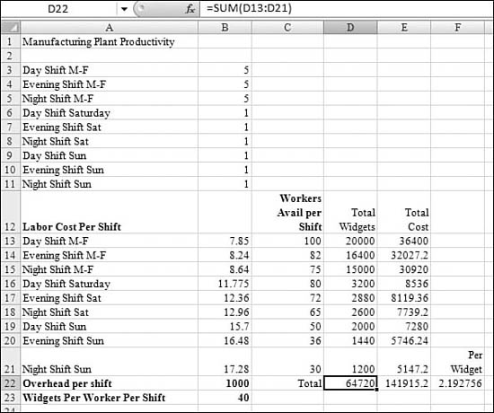
- Note that Cells B3 through B11 define how many shifts the factory will be open. All the remaining cells in the model calculate the total number of widgets produced and the average cost per widget.
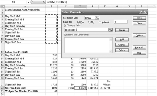
- As with Goal Seek, you start out by telling Solver that you want to set a target cell equal to a maximum, minimum, or certain value by changing other cells. For example, the Solver Parameters dialog shown in Figure 31.29 indicates that the goal is to maximize widget production by altering the number of shifts.
Figure 31.29. Maximizing widget production.
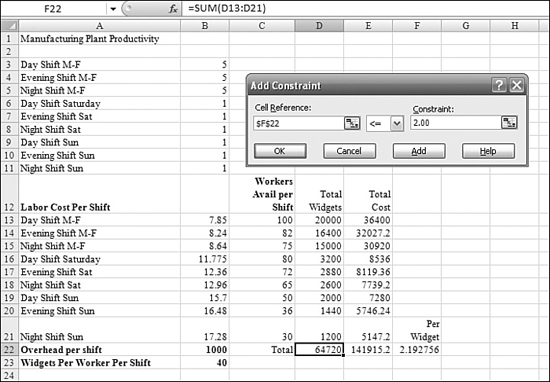
- Enter the first constraint, that the market will only bear a manufacturing cost of $2 per widget. To specify this constraint, click the Add button in the Solver Parameters dialog.
- As shown in Figure 31.30, tell Solver that the manufacturing cost must be less than or equal to $2 per widget.
Figure 31.30. Building the cost constraint.
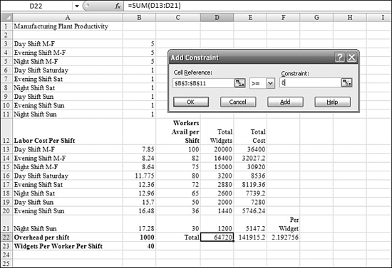
- Tell Solver that there cannot be a negative number of shifts. To do so, you need to add a constraint to indicate for each shift that the shift count must be greater than or equal to zero, as shown in Figure 31.31.
Figure 31.31. Although it is obvious to you, Solver must be told that it cannot have negative numbers of shifts.
- Specify that Cells B3:B5 must be less than or equal to five because you can have only five of each shift during the week.
- In this model, it is not valid to work 0.32 shifts; only integer values can be used in a given range. Therefore, select the value int for the comparison operator to tell Solver that a certain range can accept only integers (see Figure 31.32).
Figure 31.32. You use the integer constraint to prevent fractional answers.
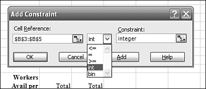
- In this case, the Saturday and Sunday shifts are a special case: The company is either open or not. The only two possible values for each cell is 0 or 1. This is a special constraint called a binary constraint. Select the bin value in the comparison operator to specify that Cells B6 through B11 are limited to binary values.
- After you have entered all the constraints, click OK to return to the Solver Parameters dialog.
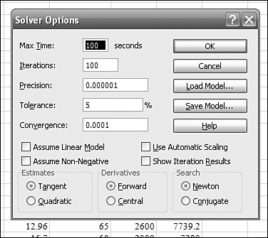
- Click the Options button on the Solver Parameters dialog to open the Solver Options dialog. Figure 31.33 shows that by default, Solver works for no more than 100 seconds. This is designed to prevent Solver from trying for a long time to find a solution.
Figure 31.33. You use the Solver Options dialog to fine-tune the processes used.
- When you have entered all the constraints and parameters, click OK to close the Solver Options dialog and return to the Solver Parameters dialog.
- Click the Solve Model button on the Solver Parameters dialog. Solver begins to iterate through possible solutions. If Solver finds a result, it reports success, as shown in Figure 31.34.
Figure 31.34. Solver reports success.
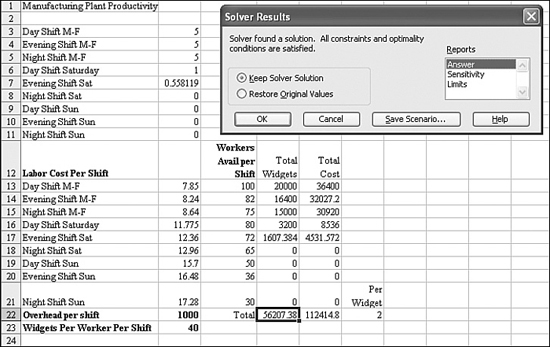
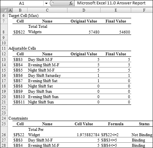
- In the Solver Results dialog, choose the Answer to have Excel provide a new worksheet that compares the original and final values. As shown in Figure 31.35, the answer report is added as a new worksheet. In the answer report, Solver tells you that you can produce 54,600 widgets by operating five of each shift during the week and one Saturday shift. The remaining shifts are not cost-effective to keep the cost per widget in Cell F22 under $2. With this current solution, the cost per widget is $1.97.
Figure 31.35. The day shift workers will be picking up some overtime on Saturdays, thanks to Solver.
You can save each Solver solution as a scenario. All these scenarios later show up in the Scenario Manager.
Excel in Practice: Emergency Room Staffing
During flu season, the hospital emergency room (ER) has an overflow of patients. Here is a line of questioning about the problem.
Q: What is the basic flow when a patient is taken to the ER?
A: The patient is assessed by a nurse. The resident sees the patient. The resident then bounces the plans off an attending.
Q: How long does the resident spend on each patient, total?
A: 15 minutes with the patient, plus 5 minutes of paperwork
Q: How long does the attending spend per patient?
A: 5 minutes with the patient, plus 5 minutes of consultation with the resident
Q: How long does the nurse spend per patient?
A: About 30 minutes
Q: How long is the typical patient in the ER?
A: 1 hour
Q: How many treatment rooms does the ER have?
A: 20 rooms
Q: What is the current staffing per shift?
A: 2 attendings, 10 nurses, and 6 residents
Given all this information, you need to build a Solver model to find a way to get more patients through the ER. To do so, here is how the model works:
- Rows 2 through 4 of the model contain the current staffing levels for residents, attendings, and nurses. These will be the input cells for Solver.
- Row 5 contains a critical constraint: There are 20 treatment rooms. Therefore, no matter how many people you staff, there cannot be more than 20 patients being seen at once.
- Rows 6 through 10 state how many minutes each resource will spend with the patient. These values are fixed in the model. You are not trying to make the doctors spend less time with the patients.
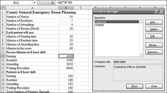
- As shown in Figure 31.36, Row 12 calculates how many minutes of nursing time are available in an 8-hour shift. The formula calculates Cell B2 × 8 hours × 60 minutes per hour. Similar formulas in Rows 13 through 15 calculate how many minutes of each other resource are available per shift.
Figure 31.36. This formula in Cell B12 calculates the number of available nursing minutes per shift.
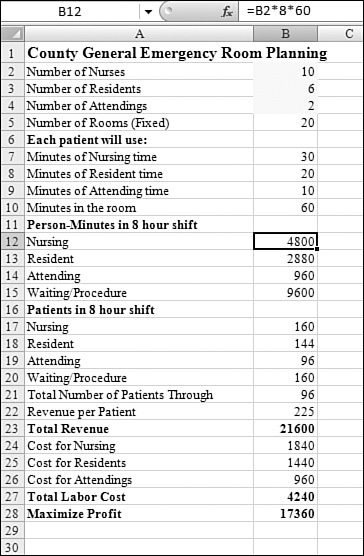
- In Row 17, if a nurse spends 30 minutes per patient, and the 10 nurses have 4,800 minutes available per shift, this means that they could potentially serve 160 patients in one shift. The formula in Cell B17 is B12/7. Similar formulas in Rows 18 through 20 calculate the process capacity for residents, attendings, and the room.
- Row 21 takes the minimum of Rows 17:20. If there is a bottleneck because of staffing, it will slow down all the other areas. At this point, the model is still trying to solve two problems: It is trying to maximize the number of patients seen while trying to make sure that there is not extra staff standing around. On the one hand, you want to maximize throughput and on the other hand, you want to minimize cost. The model takes a radical turn here, in an effort to come down to one number to represent both of these goals.
- Row 22 estimates some amount of revenue per patient.
- Row 23 calculates the total revenue.
- Rows 24 through 26 express the cost per resource per shift. Nursing costs $23 per hour, so you multiply that by 8 hours per shift and by the number of nurses in Cell B2.
- Row 27 calculates the total of the labor cost.
- Cell B28 calculates a hypothetical profit figure by subtracting labor cost from revenue. Even if these numbers aren’t exact, the model can ask Solver to maximize profit. The act of maximizing profit will seek both to get the most patients through subject to constraints and also keep the staff to a minimum.
After converting all of those words to formulas, you can have Solver try to find the optimal staffing. To do so, follow these steps:
- Start Solver.
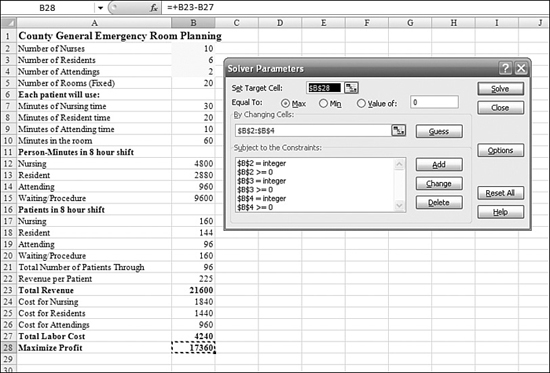
- Ask Solver to produce the maximum value in Cell B28 by changing the staffing levels in B2:B4. There are certain constraints. For example, you can’t have half a doctor cover a shift, so cells B2:B4 must be integers and must be greater than zero. (See Figure 31.37.)
Figure 31.37. Asking Solver to maximize profit while adjusting staffing levels.
In a few seconds, Solver proposes a solution. The answer report suggests that you should increase staffing by adding 1 resident and 2 attendings, as shown in Figure 31.38.
Figure 31.38. The answer report shows the optimal staffing level.
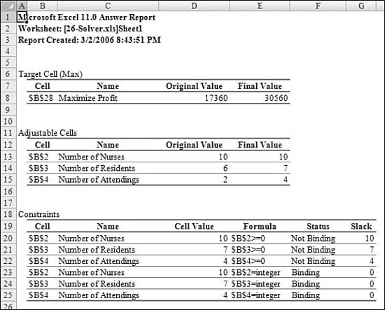
The answer report doesn’t indicate any impact on patients, but if you examine the new answers in the original sheet, as shown in Figure 31.39, you see that the patient throughput has gone from 96 to 160. The model is suggesting that the attendings, and to a lesser degree, the residents, are the bottleneck in the process. Unless you build a new wing, you can’t increase from the 20 existing treatment rooms. However, by adding staff, you can increase throughput in the existing rooms.
Figure 31.39. Patient throughput increases from 96 to 160 in the new model.