
Chapter 33. Printing
In this chapter
Using the Improved Headers and Footers 927
Using the Page Setup and Sheet Options 931
Excel 2007 offers a new Page Layout view, which is light-years ahead of the Page Break Preview mode offered in prior versions of Excel. This new view allows you to type and edit headers and footers right on the worksheet. Excel now offers support for different headers and footers on odd and even pages, and it even allows you to use a different header for the first page than for the rest of the document. Excel 2007 supports the use of color, images, and more in headers and footers.
For those who share a printer, one minor change will be major. In prior versions of Excel, if you printed 20 copies of a one-page document, Excel would send 20 print jobs to the printer. This was a huge problem if your printer sent a banner page before each print job. Finally, in Excel 2007, the software will spool all 20 pages into a single print job, eliminating the 19 extra banner pages.
Most of the major print options for controlling printing are arranged in two groups on the Page Layout ribbon. There is also a new Header & Footer Tools Design ribbon dedicated to editing headers and footers in Page Layout view.
Using Page Layout View
When you open Excel, the default view is called Normal view. In prior versions of Excel, your only choices were Normal view and Page Break Preview mode. Microsoft has added the new Page Layout view, which is perfect when you are preparing a document for printing.
In Excel 2007, the three views are available either on the Workbook Views group of the View ribbon or on the right side of the status bar, as shown in Figure 33.1.
Figure 33.1. Buttons in the status bar make Page Layout view always available.

Note
The worksheet in the figure has been zoomed to 50% in order to show multiple pages. This does not automatically happen when you enter Page Layout view.
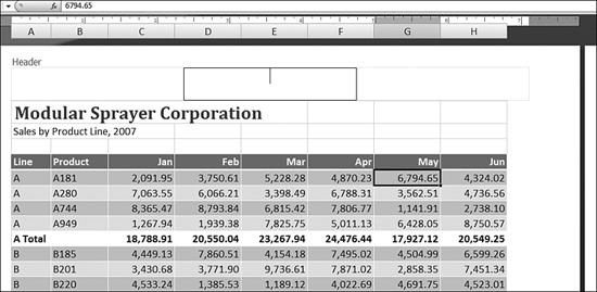
In Page Layout view, you have a fully functioning worksheet. The formula bar works. You can scroll around the worksheet as usual. However, these are the differences you’ll find when you use Page Layout view compared to using Normal view:
- Whitespace appears to show the margins on each page. You have a clear view of any page breaks between columns or rows.
- A ruler appears below the formula bar. You can change margins by dragging the gray areas of the ruler.
- Areas are marked Click to Add Header and Click to Add Footer. Whereas headers and footers are buried in previous versions of Excel, the fact that headers and footers are available is obvious in Page Layout view.
- Areas outside the data area of a worksheet are marked with Click to Add Data. One of the problems with Page Break Preview mode is that areas outside the data area were grayed out. The new Click to Add Data labels invite you to continue adding pages to your worksheet.
- The only disadvantage to Page Layout view is that Excel turns off your Freeze Panes settings in Page Layout view. Excel needs to do this in order to emphasize that Print Titles is different from Freeze Panes. It is a bit disappointing that Excel doesn’t remember the Freeze Panes settings and turn them back on when you return to Normal view. This feature will probably be added to the next version of Excel.
All in all, Page Layout view is an excellent improvement over Page Break Preview mode. It practically makes the ubiquitous Print Preview icon obsolete. Page Break Preview is still available (it is discussed later in this chapter, in the section “Working with Page Breaks”). I recommend that you try out Page Layout view when you are preparing to print.
Using the Improved Headers and Footers
In Page Layout view, Click to Add Header appears above each page. To access the new Header & Footer Tools Design ribbon, you follow these steps:
- Select View, Workbook Views, Page Layout View.
- Click the words Click to Add Header above Row 1. You should see the new Header & Footer Tools Design ribbon. Note that the insertion cursor appears in a box in the center of the header area, as shown in Figure 33.2. There are extremely faint light blue boxes around the left and right sections of the header area. You can click in any of these three boxes to add a header to the left, center, or right section of the header area.
Figure 33.2. There are three faint sections in the header: left, center, and right.
- Add either an auto header or a custom header. Details on both methods are described in the following sections.
- To format a header, you can use all the Font formatting options in the Home ribbon. You should use these formatting tools while the header is displayed.
- To exit Header/Footer mode, click in any cell of the worksheet.
![]()
To directly edit the left or right header, click to the left or right of the words Click to Add Header. When you hover over this section, a gray box appears, encouraging you to click directly in a particular section of the header.
Note
The process for adding footers is identical to the process for adding headers. Throughout the rest of this chapter, many sections describe headers. The identical instructions apply to footers.
Adding an Auto Header
For a quick header or footer, you can click the Auto Header or Auto Footer drop-down in the Header & Footer Tools Design ribbon. The drop-down offers 16 different automatic headers, including various page numbering styles, the system date, your name, the sheet name, and the file path and filename.
As shown in Figure 33.3, some of the Auto Header entries include values separated by commas. These entries put header values into the left, center, and right header sections.
Figure 33.3. To quickly add a header, you can choose from the Auto Header list.

Tip From
![]()
Although you cannot add to the Auto Header list, you can select an automatic header that is close to what you want and then customize it.
Adding a Custom Header
You can type any text you want in the three header and footer areas. One of the automatic headers says “Confidential,” but you can customize this in any way dictated by your company. No matter what type of header you need, you can type it in the header. You click in any header area and type the text that needs to be there. To start a new line, you press Enter.
To include an ampersand in the header or footer, you must use the code &&. For example, to add the header Profit & Loss, you type Profit && Loss.
Excel enables you to add several fields to a header or a footer. These fields automatically update: If you add the current date and time, the header then reflects the date and time whenever the worksheet is printed.
Icons for each field are located in the Header & Footer Elements group of the Header & Footer Tools Design ribbon. To add an element, you click in a header or footer area, position the cursor in the proper place, and click the appropriate icon in the ribbon. As long as the insertion cursor is in the header area, the screen displays the code for that field (for example, &[Date] or &[Time]). When you click in another header section, you see the current value of the autotext field.
Inserting a Picture in a Header
You can add a picture to a header or footer. It can either be a small picture that prints in the header area or a large picture that extends below the header area and acts as a watermark behind the worksheet.
To add a picture to a header, you follow these steps:
- Select View, Page Layout View.
- Click in the header area of the document.
- From the Header & Footer Tools Design ribbon, select Header & Footer Elements, Picture. Excel displays the Insert Picture dialog.
- Browse to the proper folder. Select a picture and click Insert. Excel adds the text &[Picture] to the header. You can’t actually see how large the picture will be until you click outside the header.
- Click in the spreadsheet.
- If you discover that the picture is too large, click in the header area.
- From the Header & Footer Tools Design ribbon, select Header & Footer Elements, Format Picture. The Format Picture dialog appears.
- In the Format Picture dialog, use the Size section to reduce the scale of the picture. If you use the spin button to change the height in the Scale section, the width is automatically changed as well, in order to keep the scale proportional.
- If you want your picture to appear as a watermark behind the spreadsheet, you lighten the picture. To do so, click the Picture tab of the Format Picture dialog. Change the Color drop-down to Washout.
- None of the picture items in the header feature Live Preview. To preview your picture, close the dialog box and then click outside the header. If the picture is not the way you want it, repeat steps 6 through 10 as necessary.
Using Different Headers and Footers in the Same Document
Excel 2007 allows four different header and footer scenarios:
- The same header/footer on all pages
- One header/footer on page 1 and a different header/footer on all other pages
- One header/footer on all odd pages and a different header/footer on all even pages.
- One header/footer on page 1, a second header footer on even pages, and a third header/footer on all odd pages from 3 on
Excel manages these scenarios by storing three headers for each worksheet. The first header is variously called the odd page header or the header. As you check and uncheck the options check boxes, the contents of each header remain constant, even though they might be used on different pages. Table 33.1 shows the details of each header option.
Table 33.1. Header Options

If you simply add a header in Page Layout view, it is known as the odd page header. In the default configuration, Excel displays the odd page header on all pages of the printout.
Excel has two other sets of headers that are initially hidden. One set is called the first page header. If you select Different First Page from the Options group on the Header & Footer Tools Design ribbon, Excel displays the first page header above page 1 and uses the odd page header everywhere else.
Tip From
![]()
To minimize confusion, it is best to check the Options section check boxes Different First Page and Different Odd & Even before entering headers.
Scaling Headers and Footers
Settings in the Page Layout ribbon allow you to force a worksheet to fit a certain number of pages. If the scaling options require a 75% scale on Sheet1 and a 95% scale on Sheet2, your headings are scaled as well. This causes your page numbers to appear at a different point size in various sections of the report.
Excel offers an option to force all headers and footers to print at 100% scale, regardless of the zoom for the sheet. To select this option, from the Header & Footer Tools Design ribbon, you select Options and uncheck Scale with Document.
Using the Page Setup and Sheet Options
Most of the page setup options are now in the Page Layout ribbon. The Page Setup, Scale to Fit, and Sheet Options groups reflect most of the items that used to be in the Page Setup dialog in prior versions of Excel.
Figure 33.4. Page setup options are controlled from the Page Layout ribbon.

Caution
The Background icon is out of place in the Page Setup group of the Page Layout ribbon. While every other setting in this group affects the printed page, the Background icon is only for the background on the displayed page. If you want to have a printed watermark appear behind your spreadsheet, you should use a large picture in the header, as described in the section “Inserting a Picture in a Header,” earlier in this chapter.
Adjusting Worksheet Margins
There are three methods for adjusting worksheet margins:
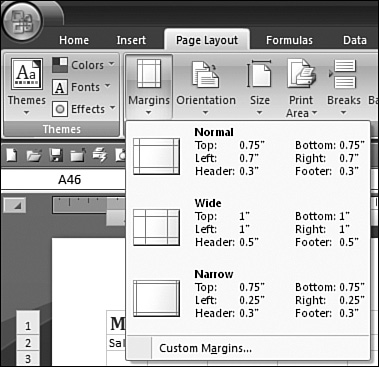
- Choose Page Layout, Margins—This drop-down offers three settings: Normal, Wide, and Narrow. To apply one of these standard setups, you simply choose from the Margins drop-down, as shown in Figure 33.5.
Figure 33.5. New in Excel 2007, you can choose a quick setting for margins.
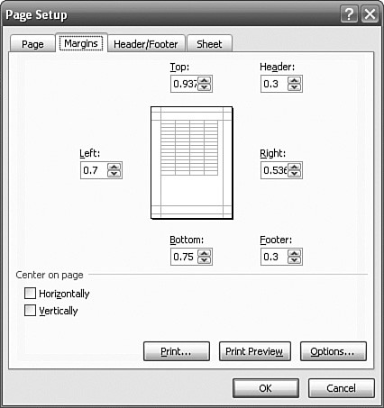
- Choose Page Layout, Page Setup, Margins, Custom Margins—You can now adjust the margins at the top, left, right, and bottom, as well as the margins for the footer and header. As shown in Figure 33.6, the dialog you use for this is the same as in legacy versions of Excel.
Figure 33.6. For control over each margin, you use the Margins tab of the Page Setup dialog.
- Choose View, Workbook Views, Page Layout View—When you do this, gray margins appear on each edge of the ruler. You can drag the gray margins in or out to decrease/increase the margins.
Adjusting Worksheet Orientation
Changing a report to print sideways (that is, landscape) now takes just a couple mouse clicks. From the Page Layout ribbon, you can select Page Setup to see the Orientation drop-down, which offers Portrait and Landscape options, as shown in Figure 33.7.
Figure 33.7. You can make a report print sideways by choosing Landscape.

Setting Worksheet Paper Size
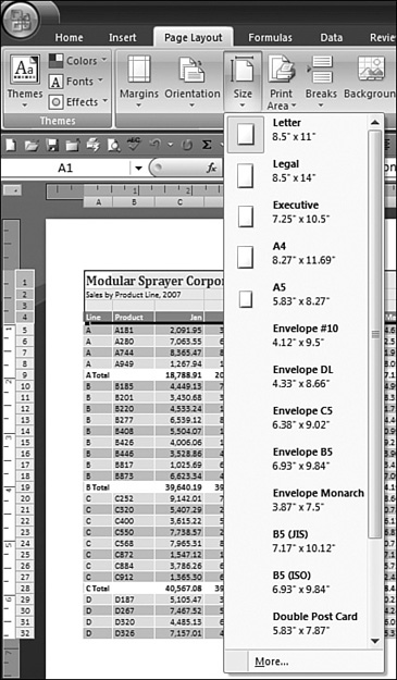
A multitude of standard paper sizes are now available from the Size drop-down in the Page Layout ribbon, as shown in Figure 33.8. You can choose one of the standard sizes or select the More menu option to specify a new size.
Figure 33.8. You can select a built-in paper size or click More to specify a custom size.
Tip From
![]()
Some paper sizes, such as 11"×17", are available only if your selected printer offers that size. If your default printer cannot print large-format paper, you should change the printer selection in the Print dialog and then return to the Page Setup dialog to select the larger-format paper.
Setting the Print Area
By default, Excel does print all the nonblank cells on a worksheet. Sometimes, you have a nicely formatted table of data to print, with some work cells in an out-of-the way location. To prevent the work cells from being printed, you follow these steps:
- Select the range of cells to be included in the print range. This might be a range of cells such as A1:Z99, or you might want to print everything in certain columns. In the latter case, your selection might be columns C:X.
- From the Page Layout ribbon, select Page Setup, Print Area, Set Print Area.
To later clear the print area and print everything on the worksheet, you can use the Clear Print Area option from the Set Print Area drop-down.
Occasionally, you will want to ignore the print areas and print everything on the worksheet. In this case, you can use the Print icon and check the box Ignore Print Areas, as shown in Figure 33.9.
Figure 33.9. To override the print area, you can choose Ignore Print Areas.

Adding Print Titles
For reports that will span more than one page, you may want the headings from the report to print at the top of each page. Although the Print Titles icon has been promoted to a large icon on the Page Layout ribbon, this command leads back to the somewhat confusing Page Layout dialog. In Figure 33.10, for example, the report is two pages wide and several pages tall. When you get to the printed page 2, there the printed report has no title or column headings. You would probably want to have the titles and column headings repeat at the top of each row.
Figure 33.10. You can use the Page Setup dialog to specify print titles to repeat on each page.
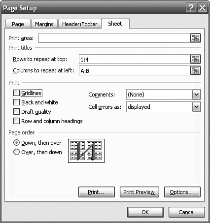
Also in Figure 33.10, the product line information from Columns A and B is considered row labels. It would be ideal if the row labels could repeat at the left side of the pages. To assign print titles, you follow these steps:
- From the Page Layout ribbon, select Page Setup, Print Titles. The Page Setup dialog appears, open to the Sheet tab.
- In the Rows to Repeat at Top box, enter the rows that should print at the top of the page. You can specify either a single row (for example, 1:1, 2:2) or a range of rows (for example, 1:4, 2:5).
- If you want columns to print at the left side of each page, enter columns in the Columns to Repeat at Left box. You can specify either a single column (for example, A:A, B:B) or multiple columns (for example, A:C, C:D).
- Click OK to return to the worksheet.
Scaling Options
You will often have worksheets in Excel that are just a few columns too wide or a few rows too long to fit on a page. Excel has had scaling options for a long time, but it is not clear on the Page Layout ribbon how the scaling options work.
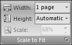
The Scale to Fit group on the Page Layout ribbon provides options for width, height, and a percentage scale. In most cases, you will either change height, width, or both to achieve the desired effect.
If your worksheet is a few columns too wide, you change the Width drop-down to specify that the worksheet should fit on one page. If you have a report that is just a bit too tall, you change the Height drop-down to specify that the worksheet should be one page tall. As shown in Figure 33.11, when you select either of these options, the Scale option is grayed out, but it still shows the scaling percentage used to make the report fit.
Figure 33.11. After you choose Scale to Fit 1 Page wide, the Scale option is grayed out but shows the actual percentage scaling used.
Tip From
![]()
If you plan on printing multiple worksheets in order to produce a printed report, you should pay attention to the scaling percentage. If Sheet1 is scaled to 77% and Sheet2 is scaled to 82%, the characters on some pages of your report will appear larger than others. You can manually set Sheet2 to 82% scaling in order to match the other worksheet.
Printing Gridlines and Headings
To print the gridlines on a worksheet, from the Page Layout ribbon, you select Sheet Options, Gridlines, Print.
You can also print the A-B-C column headings and 1-2-3 row headings. To do this, from the Page Layout ribbon, you select Sheet Options, Headings, Print. This option is great when you are printing formulas and you need to see the cell address of each cell.
Working with Page Breaks
There are two varieties of page breaks: automatic and manual.
An automatic page break occurs when Excel reaches the bottom or right margin of a physical page. These page breaks automatically change as you add rows, delete rows, or even change the height of certain rows on the page.
Initially, automatic page breaks are not shown in the worksheet. After you go to Print Preview and return to Normal view, automatic page breaks are shown in the document, using a thin dashed line. Automatic page breaks are also evident in Page Layout view and Page Break Preview mode.
Tip From
![]()
Print Preview is practically obsolete now that the Page Layout view has been added. To access the old Print Preview, you click the Office icon and then choose Print, Print Preview.
You can manually insert page breaks at rows or columns where you want to start a new page. You might want to insert a manual page break, for example, at the start of a new section in a report. A manual page break does not automatically change in response to changes in the worksheet rows.
Manually Adding Page Breaks
To manually add a page break at a certain row, you follow these steps:
- Select an entire row by clicking the row number that should be the first row on the new page. Alternatively, select Cell A in that row.
- From the Page Layout ribbon, select Page Setup, Breaks, Insert Page Break.
To manually add a page break at a certain column, you follow these steps:
- Select an entire column by clicking the number above the column that should be the first column on the new page. Alternatively, select Row 1 in that column.
- From the Page Layout ribbon, select Page Setup, Breaks, Insert Page Break.
Caution
If you insert a page break while the cell pointer is outside Row 1 or Column A, Excel simultaneously inserts a row page break and a column page break. This is rarely what you want. Make sure to select a cell in column A to insert a row break or to select a cell in row 1 to insert a column break.
Manual Versus Automatic Page Breaks
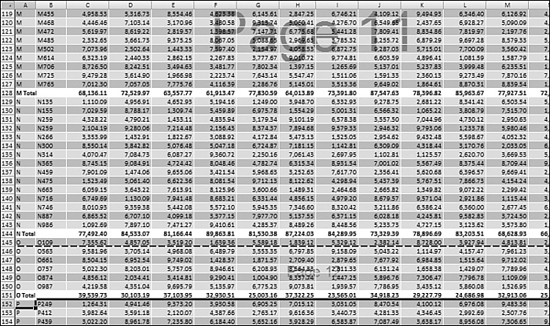
In Normal view, there is a subtle visual difference between manual and automatic page breaks. For example, in Figure 33.12, an automatic page break occurs after Row 145, and a manual page break has been inserted after Row 151. The dashed line used to indicate a manual page break is more pronounced than the line used to indicate an automatic page break.
Figure 33.12. In Normal view, the page break indicator is bolder for manual page breaks.

To see a better view of page breaks, you can select View, Page Break Preview to switch to Page Break Preview mode, as shown in Figure 33.13. In this mode, automatic page breaks are shown as dotted blue lines. Manual page breaks are shown as solid lines.
Figure 33.13. In Page Break Preview mode, automatic page breaks are shown using a dotted line and manual page breaks using a solid line.
Using Page Break Preview to Make Changes
An advantage of Page Break Preview mode is that while you are in this mode, you can move a page break by dragging the line associated with the page break. If you drag an automatic page break to expand the number of rows or columns on a page, Excel automatically changes the Scale percentage for all pages.
Removing Manual Page Breaks
To remove a manual page break for a row, you follow these steps:
- Position the cursor in the row below the page break.
- From the Page Layout ribbon, select Page Setup, Breaks, Remove Page Break.
To remove a manual page break for a column, you follow these steps:
- Position the cursor in the column to the right of the page break.
- From the Page Layout ribbon, select Page Setup, Breaks, Remove Page Break.
To remove all manual page breaks, from the Page Layout ribbon, you select Page Setup, Breaks, Reset All Page Breaks.
Printing
There are two methods for printing. You can click the Quick Print icon to send one copy of the active sheet to the currently selected printer. For additional control over the printer, number of copies, or the worksheet to print, you can use the Print dialog box.
Choosing Quick Print
To send a copy of the worksheet to the active printer, you can click the Office icon and then choose Print, Quick Print. The Quick Print icon is usually available in your Quick Access toolbar, unless someone has customized the toolbar and removed the icon. See Chapter 2 for information on customizing the toolbar.
Controlling Print Options by Using the Print Dialog Box
To access additional printing options, you can use the Print dialog box, shown in Figure 33.14. To open this dialog, you select the Office icon and then choose Print.
Figure 33.14. Additional printing options can be controlled in the Print dialog.
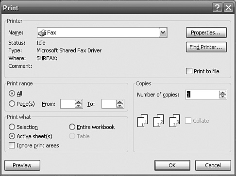
In the Print dialog, the Name drop-down lists all the available printers. To print to a different printer, you select a printer from this drop-down.
By default, Excel prints the entire print range. To print specific pages, you use the From and To spin buttons. To print more than one copy of the document, you can change the Copies spin button. If you select more than one copy, you can select the Collate check box. If Collate is turned on, Excel prints pages 1, 2, 3, 1, 2, 3, 1, 2, 3, and so on. If Collate is turned off, Excel prints pages 1, 1, 1, 2, 2, 2, 3, 3, 3, and so on.
The Print What section of the Print dialog offers five choices:
- Selection—You should choose this option to override the print area and print only the selected range of data.
- Active Sheet(s)—This is the default. When it is selected, Excel prints the print area on each selected sheet.
- Entire Workbook—When this option is selected, Excel prints the print area on all visible sheets in the workbook.
- Table—When this option is selected, Excel prints the current table.
- Ignore Print Areas—This check box works in conjunction with Active Sheet(s) and Entire Workbook. If your print area is set up to define a subset of the worksheet as the print area, choosing Ignore Print Area causes the entire workbook to be printed.
Controlling Printer Options
Depending on your printer model, there may be additional print settings available. Although Excel does not control these values, there is a button that allows you to access your printer’s options panel. To use this button, you follow these steps:
- Select the Office icon and then choose Print. The Print dialog appears.
- In the Print dialog, near the Printer Name drop-down, click choose the Properties button. The Printer Options dialog for your particular printer appears. This dialog varies, depending on your printer. Its available settings might include color adjustments, toner usage, and more.