
Basic Design Theory
Abstract
The performance—thrust or power, fuel consumption, temperatures, shaft speeds, etc.—of a gas turbine engine is crucially dependent upon its inlet and exit conditions. The full range of inlet conditions that a given gas turbine engine application could encounter is encompassed in the operational envelope. This comprises an environmental envelope, defining ambient pressure, temperature, and humidity; installation pressure losses; and a flight envelope for aircraft engines. The environmental envelope for an engine defines the range of ambient pressure (or pressure altitude), ambient temperature, and humidity throughout which it must operate satisfactorily.
Keywords
Basic design theory; operational envelope; design point; performance; inlet and exit conditions; gas properties; thermodynamics
“Never mistake motion for action.”
—Ernest Hemingway
At some point, a gas turbine operations or repair and overhaul engineer has to consider the design of the gas turbine package in his or her care. This may be for:
Regardless of the reason for a look at the gas turbine system design, it is useful to know the terminology and basic theory behind the OEM’s design. What follows is a summary of an OEM’s basic theory and terminology in the design areas of:
After these sections, there are two case studies and a Mach number/altitude chart developed by an aircraft engine designer.
The very basic thermodynamic laws and cycle diagrams used by operational engineers with little or no design (retrofit or otherwise) or specification responsibility are in the chapter on gas turbine cycles.
Operational Envelope1
The performance—thrust or power, fuel consumption, temperatures, shaft speeds, etc.—of a gas turbine engine is crucially dependent upon its inlet and exit conditions. The most important items are pressure and temperature, which are determined by the combination of ambient values and any changes due to flight speed, or pressure loss imposed by the installation.
The full range of inlet conditions that a given gas turbine engine application could encounter is encompassed in the operational envelope. This comprises:
• An environmental envelope, defining ambient pressure, temperature, and humidity
The Environmental Envelope
The environmental envelope for an engine defines the range of ambient pressure (or pressure altitude), ambient temperature, and humidity throughout which it must operate satisfactorily. These atmospheric conditions local to the engine have a considerable effect upon its performance.
International Standards
The International Standard Atmosphere (ISA) defines standard day ambient temperature and pressure up to an altitude of 30,500 m (100,066 ft). The term ISA conditions alone would imply zero relative humidity.
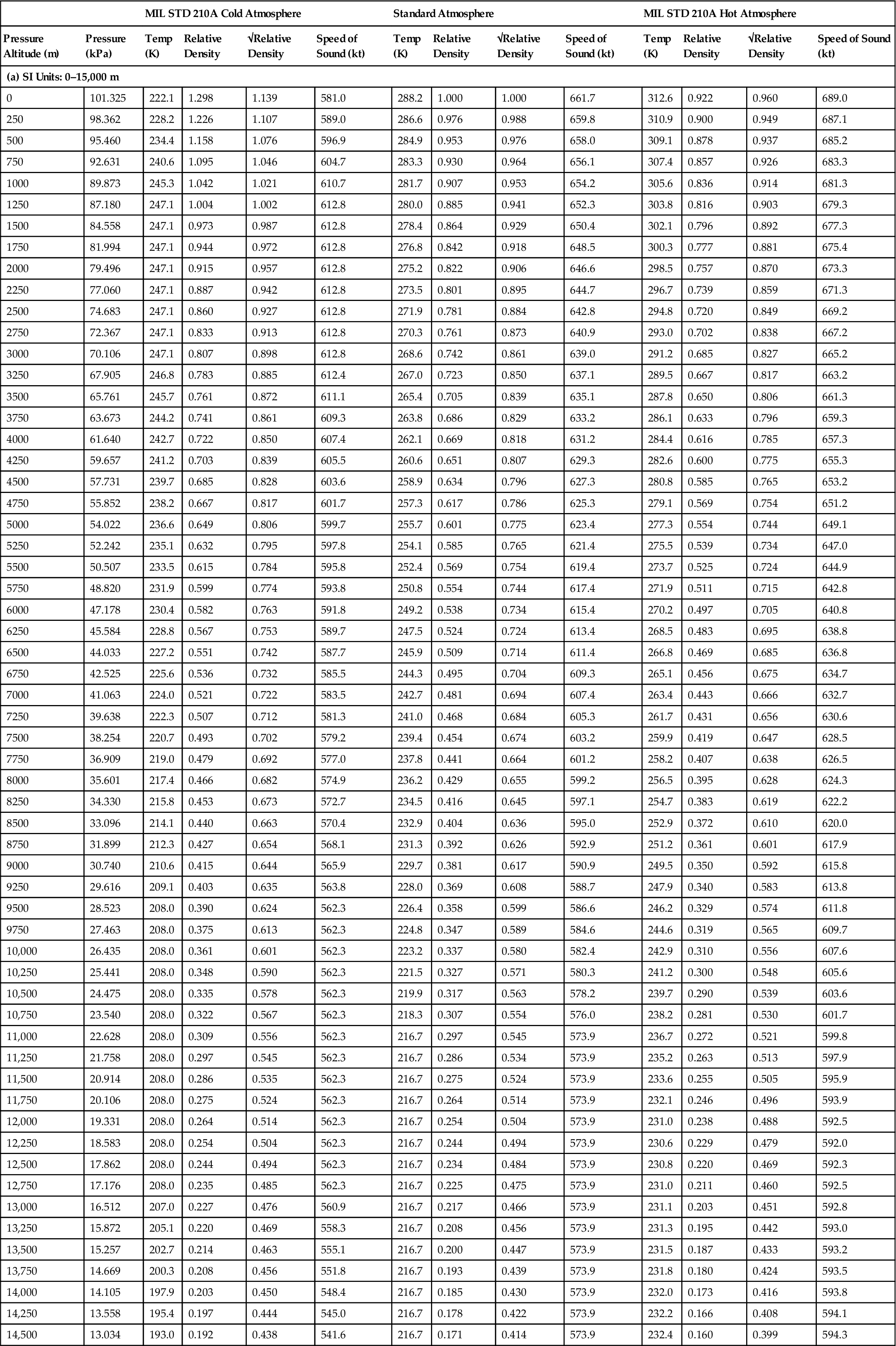
US Military Standard 210 (MIL 210) is the most commonly used standard for defining likely extremes of ambient temperature versus altitude. This is primarily an aerospace standard, and is also widely used for land-based applications though with the hot and cold day temperature ranges extended. Table 19–1 shows the ambient pressure and temperature relationships of MIL 210 and ISA.
TABLE 19–1
Ambient Conditions Versus Pressure Altitude
| MIL STD 210A Cold Atmosphere | Standard Atmosphere | MIL STD 210A Hot Atmosphere | |||||||||||
| Pressure Altitude (m) | Pressure (kPa) | Temp (K) | Relative Density | √Relative Density | Speed of Sound (kt) | Temp (K) | Relative Density | √Relative Density | Speed of Sound (kt) | Temp (K) | Relative Density | √Relative Density | Speed of Sound (kt) |
| (a) SI Units: 0–15,000 m | |||||||||||||
| 0 | 101.325 | 222.1 | 1.298 | 1.139 | 581.0 | 288.2 | 1.000 | 1.000 | 661.7 | 312.6 | 0.922 | 0.960 | 689.0 |
| 250 | 98.362 | 228.2 | 1.226 | 1.107 | 589.0 | 286.6 | 0.976 | 0.988 | 659.8 | 310.9 | 0.900 | 0.949 | 687.1 |
| 500 | 95.460 | 234.4 | 1.158 | 1.076 | 596.9 | 284.9 | 0.953 | 0.976 | 658.0 | 309.1 | 0.878 | 0.937 | 685.2 |
| 750 | 92.631 | 240.6 | 1.095 | 1.046 | 604.7 | 283.3 | 0.930 | 0.964 | 656.1 | 307.4 | 0.857 | 0.926 | 683.3 |
| 1000 | 89.873 | 245.3 | 1.042 | 1.021 | 610.7 | 281.7 | 0.907 | 0.953 | 654.2 | 305.6 | 0.836 | 0.914 | 681.3 |
| 1250 | 87.180 | 247.1 | 1.004 | 1.002 | 612.8 | 280.0 | 0.885 | 0.941 | 652.3 | 303.8 | 0.816 | 0.903 | 679.3 |
| 1500 | 84.558 | 247.1 | 0.973 | 0.987 | 612.8 | 278.4 | 0.864 | 0.929 | 650.4 | 302.1 | 0.796 | 0.892 | 677.3 |
| 1750 | 81.994 | 247.1 | 0.944 | 0.972 | 612.8 | 276.8 | 0.842 | 0.918 | 648.5 | 300.3 | 0.777 | 0.881 | 675.4 |
| 2000 | 79.496 | 247.1 | 0.915 | 0.957 | 612.8 | 275.2 | 0.822 | 0.906 | 646.6 | 298.5 | 0.757 | 0.870 | 673.3 |
| 2250 | 77.060 | 247.1 | 0.887 | 0.942 | 612.8 | 273.5 | 0.801 | 0.895 | 644.7 | 296.7 | 0.739 | 0.859 | 671.3 |
| 2500 | 74.683 | 247.1 | 0.860 | 0.927 | 612.8 | 271.9 | 0.781 | 0.884 | 642.8 | 294.8 | 0.720 | 0.849 | 669.2 |
| 2750 | 72.367 | 247.1 | 0.833 | 0.913 | 612.8 | 270.3 | 0.761 | 0.873 | 640.9 | 293.0 | 0.702 | 0.838 | 667.2 |
| 3000 | 70.106 | 247.1 | 0.807 | 0.898 | 612.8 | 268.6 | 0.742 | 0.861 | 639.0 | 291.2 | 0.685 | 0.827 | 665.2 |
| 3250 | 67.905 | 246.8 | 0.783 | 0.885 | 612.4 | 267.0 | 0.723 | 0.850 | 637.1 | 289.5 | 0.667 | 0.817 | 663.2 |
| 3500 | 65.761 | 245.7 | 0.761 | 0.872 | 611.1 | 265.4 | 0.705 | 0.839 | 635.1 | 287.8 | 0.650 | 0.806 | 661.3 |
| 3750 | 63.673 | 244.2 | 0.741 | 0.861 | 609.3 | 263.8 | 0.686 | 0.829 | 633.2 | 286.1 | 0.633 | 0.796 | 659.3 |
| 4000 | 61.640 | 242.7 | 0.722 | 0.850 | 607.4 | 262.1 | 0.669 | 0.818 | 631.2 | 284.4 | 0.616 | 0.785 | 657.3 |
| 4250 | 59.657 | 241.2 | 0.703 | 0.839 | 605.5 | 260.6 | 0.651 | 0.807 | 629.3 | 282.6 | 0.600 | 0.775 | 655.3 |
| 4500 | 57.731 | 239.7 | 0.685 | 0.828 | 603.6 | 258.9 | 0.634 | 0.796 | 627.3 | 280.8 | 0.585 | 0.765 | 653.2 |
| 4750 | 55.852 | 238.2 | 0.667 | 0.817 | 601.7 | 257.3 | 0.617 | 0.786 | 625.3 | 279.1 | 0.569 | 0.754 | 651.2 |
| 5000 | 54.022 | 236.6 | 0.649 | 0.806 | 599.7 | 255.7 | 0.601 | 0.775 | 623.4 | 277.3 | 0.554 | 0.744 | 649.1 |
| 5250 | 52.242 | 235.1 | 0.632 | 0.795 | 597.8 | 254.1 | 0.585 | 0.765 | 621.4 | 275.5 | 0.539 | 0.734 | 647.0 |
| 5500 | 50.507 | 233.5 | 0.615 | 0.784 | 595.8 | 252.4 | 0.569 | 0.754 | 619.4 | 273.7 | 0.525 | 0.724 | 644.9 |
| 5750 | 48.820 | 231.9 | 0.599 | 0.774 | 593.8 | 250.8 | 0.554 | 0.744 | 617.4 | 271.9 | 0.511 | 0.715 | 642.8 |
| 6000 | 47.178 | 230.4 | 0.582 | 0.763 | 591.8 | 249.2 | 0.538 | 0.734 | 615.4 | 270.2 | 0.497 | 0.705 | 640.8 |
| 6250 | 45.584 | 228.8 | 0.567 | 0.753 | 589.7 | 247.5 | 0.524 | 0.724 | 613.4 | 268.5 | 0.483 | 0.695 | 638.8 |
| 6500 | 44.033 | 227.2 | 0.551 | 0.742 | 587.7 | 245.9 | 0.509 | 0.714 | 611.4 | 266.8 | 0.469 | 0.685 | 636.8 |
| 6750 | 42.525 | 225.6 | 0.536 | 0.732 | 585.5 | 244.3 | 0.495 | 0.704 | 609.3 | 265.1 | 0.456 | 0.675 | 634.7 |
| 7000 | 41.063 | 224.0 | 0.521 | 0.722 | 583.5 | 242.7 | 0.481 | 0.694 | 607.4 | 263.4 | 0.443 | 0.666 | 632.7 |
| 7250 | 39.638 | 222.3 | 0.507 | 0.712 | 581.3 | 241.0 | 0.468 | 0.684 | 605.3 | 261.7 | 0.431 | 0.656 | 630.6 |
| 7500 | 38.254 | 220.7 | 0.493 | 0.702 | 579.2 | 239.4 | 0.454 | 0.674 | 603.2 | 259.9 | 0.419 | 0.647 | 628.5 |
| 7750 | 36.909 | 219.0 | 0.479 | 0.692 | 577.0 | 237.8 | 0.441 | 0.664 | 601.2 | 258.2 | 0.407 | 0.638 | 626.5 |
| 8000 | 35.601 | 217.4 | 0.466 | 0.682 | 574.9 | 236.2 | 0.429 | 0.655 | 599.2 | 256.5 | 0.395 | 0.628 | 624.3 |
| 8250 | 34.330 | 215.8 | 0.453 | 0.673 | 572.7 | 234.5 | 0.416 | 0.645 | 597.1 | 254.7 | 0.383 | 0.619 | 622.2 |
| 8500 | 33.096 | 214.1 | 0.440 | 0.663 | 570.4 | 232.9 | 0.404 | 0.636 | 595.0 | 252.9 | 0.372 | 0.610 | 620.0 |
| 8750 | 31.899 | 212.3 | 0.427 | 0.654 | 568.1 | 231.3 | 0.392 | 0.626 | 592.9 | 251.2 | 0.361 | 0.601 | 617.9 |
| 9000 | 30.740 | 210.6 | 0.415 | 0.644 | 565.9 | 229.7 | 0.381 | 0.617 | 590.9 | 249.5 | 0.350 | 0.592 | 615.8 |
| 9250 | 29.616 | 209.1 | 0.403 | 0.635 | 563.8 | 228.0 | 0.369 | 0.608 | 588.7 | 247.9 | 0.340 | 0.583 | 613.8 |
| 9500 | 28.523 | 208.0 | 0.390 | 0.624 | 562.3 | 226.4 | 0.358 | 0.599 | 586.6 | 246.2 | 0.329 | 0.574 | 611.8 |
| 9750 | 27.463 | 208.0 | 0.375 | 0.613 | 562.3 | 224.8 | 0.347 | 0.589 | 584.6 | 244.6 | 0.319 | 0.565 | 609.7 |
| 10,000 | 26.435 | 208.0 | 0.361 | 0.601 | 562.3 | 223.2 | 0.337 | 0.580 | 582.4 | 242.9 | 0.310 | 0.556 | 607.6 |
| 10,250 | 25.441 | 208.0 | 0.348 | 0.590 | 562.3 | 221.5 | 0.327 | 0.571 | 580.3 | 241.2 | 0.300 | 0.548 | 605.6 |
| 10,500 | 24.475 | 208.0 | 0.335 | 0.578 | 562.3 | 219.9 | 0.317 | 0.563 | 578.2 | 239.7 | 0.290 | 0.539 | 603.6 |
| 10,750 | 23.540 | 208.0 | 0.322 | 0.567 | 562.3 | 218.3 | 0.307 | 0.554 | 576.0 | 238.2 | 0.281 | 0.530 | 601.7 |
| 11,000 | 22.628 | 208.0 | 0.309 | 0.556 | 562.3 | 216.7 | 0.297 | 0.545 | 573.9 | 236.7 | 0.272 | 0.521 | 599.8 |
| 11,250 | 21.758 | 208.0 | 0.297 | 0.545 | 562.3 | 216.7 | 0.286 | 0.534 | 573.9 | 235.2 | 0.263 | 0.513 | 597.9 |
| 11,500 | 20.914 | 208.0 | 0.286 | 0.535 | 562.3 | 216.7 | 0.275 | 0.524 | 573.9 | 233.6 | 0.255 | 0.505 | 595.9 |
| 11,750 | 20.106 | 208.0 | 0.275 | 0.524 | 562.3 | 216.7 | 0.264 | 0.514 | 573.9 | 232.1 | 0.246 | 0.496 | 593.9 |
| 12,000 | 19.331 | 208.0 | 0.264 | 0.514 | 562.3 | 216.7 | 0.254 | 0.504 | 573.9 | 231.0 | 0.238 | 0.488 | 592.5 |
| 12,250 | 18.583 | 208.0 | 0.254 | 0.504 | 562.3 | 216.7 | 0.244 | 0.494 | 573.9 | 230.6 | 0.229 | 0.479 | 592.0 |
| 12,500 | 17.862 | 208.0 | 0.244 | 0.494 | 562.3 | 216.7 | 0.234 | 0.484 | 573.9 | 230.8 | 0.220 | 0.469 | 592.3 |
| 12,750 | 17.176 | 208.0 | 0.235 | 0.485 | 562.3 | 216.7 | 0.225 | 0.475 | 573.9 | 231.0 | 0.211 | 0.460 | 592.5 |
| 13,000 | 16.512 | 207.0 | 0.227 | 0.476 | 560.9 | 216.7 | 0.217 | 0.466 | 573.9 | 231.1 | 0.203 | 0.451 | 592.8 |
| 13,250 | 15.872 | 205.1 | 0.220 | 0.469 | 558.3 | 216.7 | 0.208 | 0.456 | 573.9 | 231.3 | 0.195 | 0.442 | 593.0 |
| 13,500 | 15.257 | 202.7 | 0.214 | 0.463 | 555.1 | 216.7 | 0.200 | 0.447 | 573.9 | 231.5 | 0.187 | 0.433 | 593.2 |
| 13,750 | 14.669 | 200.3 | 0.208 | 0.456 | 551.8 | 216.7 | 0.193 | 0.439 | 573.9 | 231.8 | 0.180 | 0.424 | 593.5 |
| 14,000 | 14.105 | 197.9 | 0.203 | 0.450 | 548.4 | 216.7 | 0.185 | 0.430 | 573.9 | 232.0 | 0.173 | 0.416 | 593.8 |
| 14,250 | 13.558 | 195.4 | 0.197 | 0.444 | 545.0 | 216.7 | 0.178 | 0.422 | 573.9 | 232.2 | 0.166 | 0.408 | 594.1 |
| 14,500 | 13.034 | 193.0 | 0.192 | 0.438 | 541.6 | 216.7 | 0.171 | 0.414 | 573.9 | 232.4 | 0.160 | 0.399 | 594.3 |
| 14,750 | 12.530 | 190.7 | 0.187 | 0.432 | 538.4 | 216.7 | 0.164 | 0.406 | 573.9 | 232.6 | 0.153 | 0.391 | 594.6 |
| 15,000 | 12.045 | 188.7 | 0.182 | 0.426 | 535.6 | 216.7 | 0.158 | 0.398 | 573.9 | 232.8 | 0.147 | 0.384 | 594.9 |
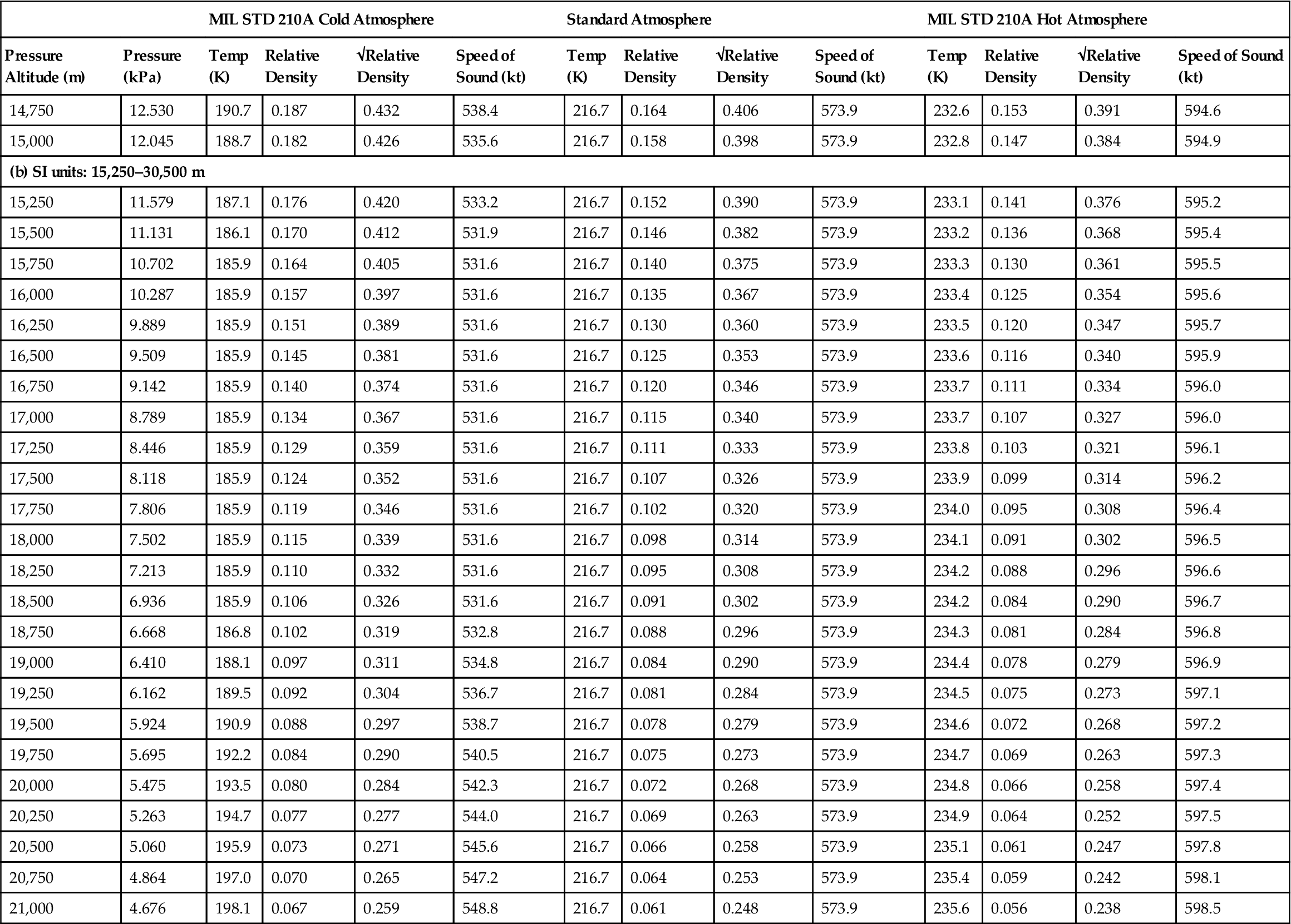
| (b) SI units: 15,250–30,500 m | |||||||||||||
| 15,250 | 11.579 | 187.1 | 0.176 | 0.420 | 533.2 | 216.7 | 0.152 | 0.390 | 573.9 | 233.1 | 0.141 | 0.376 | 595.2 |
| 15,500 | 11.131 | 186.1 | 0.170 | 0.412 | 531.9 | 216.7 | 0.146 | 0.382 | 573.9 | 233.2 | 0.136 | 0.368 | 595.4 |
| 15,750 | 10.702 | 185.9 | 0.164 | 0.405 | 531.6 | 216.7 | 0.140 | 0.375 | 573.9 | 233.3 | 0.130 | 0.361 | 595.5 |
| 16,000 | 10.287 | 185.9 | 0.157 | 0.397 | 531.6 | 216.7 | 0.135 | 0.367 | 573.9 | 233.4 | 0.125 | 0.354 | 595.6 |
| 16,250 | 9.889 | 185.9 | 0.151 | 0.389 | 531.6 | 216.7 | 0.130 | 0.360 | 573.9 | 233.5 | 0.120 | 0.347 | 595.7 |
| 16,500 | 9.509 | 185.9 | 0.145 | 0.381 | 531.6 | 216.7 | 0.125 | 0.353 | 573.9 | 233.6 | 0.116 | 0.340 | 595.9 |
| 16,750 | 9.142 | 185.9 | 0.140 | 0.374 | 531.6 | 216.7 | 0.120 | 0.346 | 573.9 | 233.7 | 0.111 | 0.334 | 596.0 |
| 17,000 | 8.789 | 185.9 | 0.134 | 0.367 | 531.6 | 216.7 | 0.115 | 0.340 | 573.9 | 233.7 | 0.107 | 0.327 | 596.0 |
| 17,250 | 8.446 | 185.9 | 0.129 | 0.359 | 531.6 | 216.7 | 0.111 | 0.333 | 573.9 | 233.8 | 0.103 | 0.321 | 596.1 |
| 17,500 | 8.118 | 185.9 | 0.124 | 0.352 | 531.6 | 216.7 | 0.107 | 0.326 | 573.9 | 233.9 | 0.099 | 0.314 | 596.2 |
| 17,750 | 7.806 | 185.9 | 0.119 | 0.346 | 531.6 | 216.7 | 0.102 | 0.320 | 573.9 | 234.0 | 0.095 | 0.308 | 596.4 |
| 18,000 | 7.502 | 185.9 | 0.115 | 0.339 | 531.6 | 216.7 | 0.098 | 0.314 | 573.9 | 234.1 | 0.091 | 0.302 | 596.5 |
| 18,250 | 7.213 | 185.9 | 0.110 | 0.332 | 531.6 | 216.7 | 0.095 | 0.308 | 573.9 | 234.2 | 0.088 | 0.296 | 596.6 |
| 18,500 | 6.936 | 185.9 | 0.106 | 0.326 | 531.6 | 216.7 | 0.091 | 0.302 | 573.9 | 234.2 | 0.084 | 0.290 | 596.7 |
| 18,750 | 6.668 | 186.8 | 0.102 | 0.319 | 532.8 | 216.7 | 0.088 | 0.296 | 573.9 | 234.3 | 0.081 | 0.284 | 596.8 |
| 19,000 | 6.410 | 188.1 | 0.097 | 0.311 | 534.8 | 216.7 | 0.084 | 0.290 | 573.9 | 234.4 | 0.078 | 0.279 | 596.9 |
| 19,250 | 6.162 | 189.5 | 0.092 | 0.304 | 536.7 | 216.7 | 0.081 | 0.284 | 573.9 | 234.5 | 0.075 | 0.273 | 597.1 |
| 19,500 | 5.924 | 190.9 | 0.088 | 0.297 | 538.7 | 216.7 | 0.078 | 0.279 | 573.9 | 234.6 | 0.072 | 0.268 | 597.2 |
| 19,750 | 5.695 | 192.2 | 0.084 | 0.290 | 540.5 | 216.7 | 0.075 | 0.273 | 573.9 | 234.7 | 0.069 | 0.263 | 597.3 |
| 20,000 | 5.475 | 193.5 | 0.080 | 0.284 | 542.3 | 216.7 | 0.072 | 0.268 | 573.9 | 234.8 | 0.066 | 0.258 | 597.4 |
| 20,250 | 5.263 | 194.7 | 0.077 | 0.277 | 544.0 | 216.7 | 0.069 | 0.263 | 573.9 | 234.9 | 0.064 | 0.252 | 597.5 |
| 20,500 | 5.060 | 195.9 | 0.073 | 0.271 | 545.6 | 216.7 | 0.066 | 0.258 | 573.9 | 235.1 | 0.061 | 0.247 | 597.8 |
| 20,750 | 4.864 | 197.0 | 0.070 | 0.265 | 547.2 | 216.7 | 0.064 | 0.253 | 573.9 | 235.4 | 0.059 | 0.242 | 598.1 |
| 21,000 | 4.676 | 198.1 | 0.067 | 0.259 | 548.8 | 216.7 | 0.061 | 0.248 | 573.9 | 235.6 | 0.056 | 0.238 | 598.5 |
Notes: The source for this chart provides data for up to 100,200 m pressure altitude.
To convert kt to m/s multiply by 0.5144.
To convert kt to km/h multiply by 1.8520.
To convert K to °C subtract 273.15.
To convert K to °R multiply by 1.8.
To convert K to °F multiply by 1.8 and subtract 459.67.
Density at ISA sea level static = 1.2250 kg/m3.
Standard practice is to interpolate linearly between altitudes listed.
(Source: Rolls Royce.)
For land-based engines, performance data are frequently quoted at the single point ISO conditions, as stipulated by the International Organization for Standardization (ISO). These are:
Ambient Pressure and Pressure Altitude
Pressure altitude, or geo-potential altitude, at a point in the atmosphere is defined by the level of ambient pressure, as per the International Standard Atmosphere. Pressure altitude is therefore not set by the elevation of the point in question above sea level. For example, due to prevailing weather conditions a ship at sea may encounter a low ambient pressure of, say, 97.8 kPa, and hence its pressure altitude would be 300 m.
Table 19–1 includes the ISA definition of pressure altitude versus ambient pressure, and Figure 19–1 shows the relationship graphically. It will be observed that pressure falls exponentially from its sea level value of 101.325 kPa (14.696 psia) to 1.08 kPa (0.16 psia) at 30,500 m (100,066 ft).
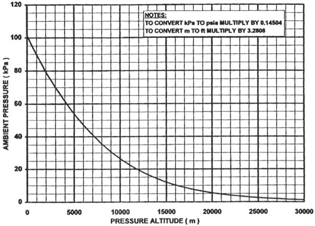
The highest value of ambient pressure for which an engine would be designed is 108 kPa (15.7 psia). This would be due to local conditions and is commensurate with a pressure altitude of –600 m (–1968 ft).
Ambient Temperature
Table 19–1 also presents the ISA standard day ambient temperature, together with MIL 210 cold and hot day temperature, versus pressure altitude. Figure 19–2 shows these three lines of ambient temperature plotted versus pressure altitude.
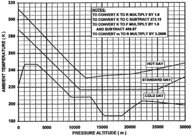
Standard day temperature falls at the rate of approximately 6°C per 1000 m (2°C for 1000 ft) until a pressure altitude of 11,000 m (36,089 ft), after which it stays constant until 25,000 m (82,000 ft). This altitude of 11,000 m is referred to as the tropopause; the region below this is the troposphere, and that above it is the stratosphere. Above 25,000 m standard day temperature rises again.
The minimum MIL 210 cold day temperature of 185.9 K (–87.3°C) occurs between 15,545 m (51,000 ft) and 18,595 m (61,000 ft). The maximum MIL 210 hot day temperature is 312.6 K (39.5°C) at sea level.
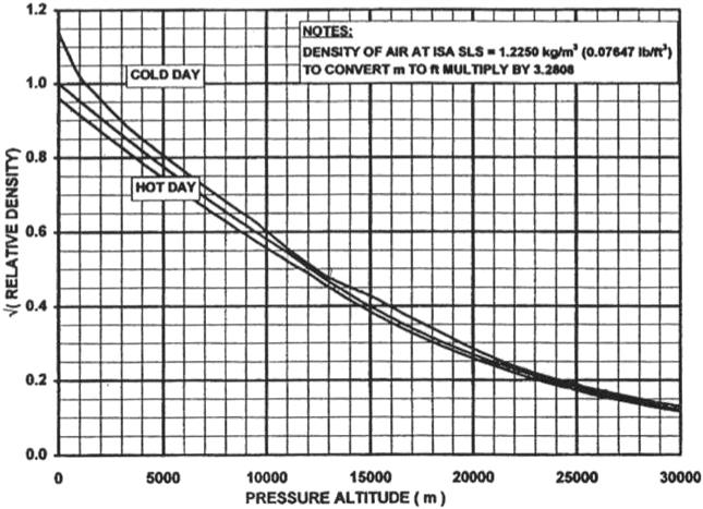
Relative Density and the Speed of Sound
Relative density is the atmospheric density divided by that for an ISA standard day at sea level. Table 19–1 includes relative density, the square root of relative density, and the speed of sound for cold, hot and standard days. Figures 19–3 through 19–5 present this data graphically. These parameters are important in understanding the interrelationships between the different definitions of flight speed.
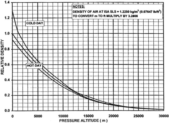

Density falls with pressure altitude such that at 30,500 m (100,066 ft) it is only 1.3% of its sISA sea level value. The maximum speed of sound of 689.0 kt (1276 km/h, 792.8 mph) occurs on a hot day at sea level. The minimum value is 531.6 kt (984.3 km/h, 611.6 mph), occurring between 15,545 m (51,000 ft) and 18,595 m (61,000 ft).
Specific and Relative Humidity
Atmospheric specific humidity is variously defined either as:
The former definition is used exclusively herein; for most practical purposes the difference is small anyway. Relative humidity is specific humidity divided by the saturated value for the prevailing ambient pressure and temperature.
Humidity has the least powerful effect upon engine performance of the three ambient parameters. Its effect is not negligible, however, in that it changes the inlet air’s molecular weight, and hence basic properties of specific heat and gas constant. In addition, condensation may occasionally have gross effects on temperature. Wherever possible humidity effects should be considered, particularly for hot days with high levels of relative humidity.
For most gas turbine performance purposes, specific humidity is negligible below 0°C, and also above 40°C. The latter is because the highest temperatures only occur in desert conditions, where water is scarce. MIL 210 gives 35°C as the highest ambient temperature at which to consider 100% relative humidity.
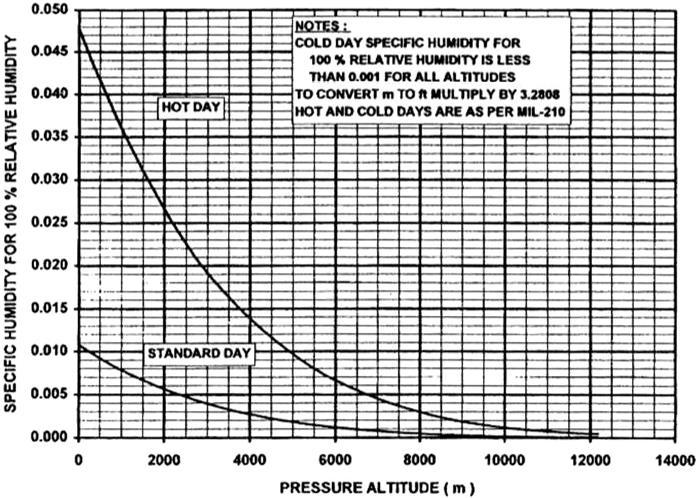
Figure 19–6 presents specific humidity for 100% relative humidity versus pressure altitude for cold, standard, and hot days. For MIL 210 cold days specific humidity is almost zero for all altitudes. The maximum specific humidity will never exceed 4.8%, which would occur on a MIL 210 hot day at sea level. In the troposphere (i.e., below 11,000 m) specific humidity for 100% relative humidity falls with pressure altitude, due to the falling ambient temperature. Above that, in the stratosphere, water vapor content is negligible, almost all having condensed out at the colder temperatures below.
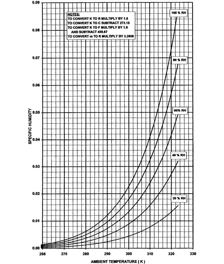
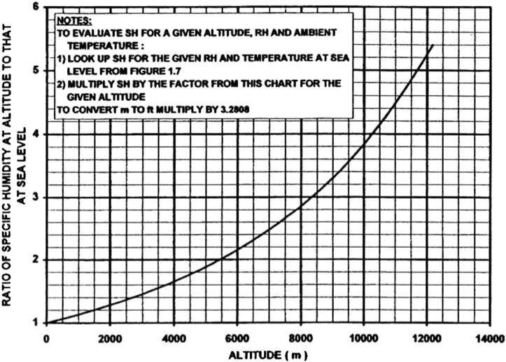
Figures 19–7 and 19–8 facilitate conversion of specific and relative humidities. Figure 19–7 presents specific humidity versus ambient temperature and relative humidity at sea level. For other altitudes Figure 19–8 presents factors to be applied to the specific humidity obtained from Figure 19–7. For a given relative humidity specific humidity is higher at altitude because whereas water vapor pressure is dependent only on temperature, air pressure is significantly lower.
Industrial Gas Turbines
The environmental envelope for industrial gas turbines, both for power generation and mechanical drive applications, is normally taken from Table 19–1 up to a pressure altitude of around 4500 m (or 15,000 ft). Hot and cold day ambient temperatures beyond those of MIL 210 are often used, ±50°C being typical at sea level. For specific fixed locations, altitude is known, and S curves are available defining the annual distribution of ambient temperature: these allow lifing assessments and rating selection. (The name derives from the characteristic shape of the curve, which plots the percentage of time for which a particular temperature level would be exceeded.)
The range of specific humidities for an industrial gas turbine would be commensurate with 0–100% relative humidity over most of the ambient temperature range, with some alleviation at the hot and cold extremes.
Automotive Gas Turbines
Most comments are as per industrial engines, except that narrowing down the range of ambient conditions for a specific application based on a fixed location is not appropriate.
Marine Gas Turbines
The range of pressure altitudes at sea is governed by weather conditions only, as the element of elevation that significantly affects all other gas turbine types is absent. The practice of the US Navy, the most prolific user of marine gas turbines, is to take the likely range of ambient pressure as 87–108 kPa (12.6–15.7 psia). This corresponds to a pressure altitude variation of –600–1800 m (–1968–5905 ft).
At sea, free stream air temperature (i.e., that not affected by solar heating of the ship’s decks) matches sea surface temperature, day or night. Owing to the vast thermal inertia of the sea there is a significant reduction in the range of ambient temperature that marine gas turbines encounter when on the open sea relative to land based or aircraft gas turbines. However, ships must also be able to operate close to land, including polar ice fields and the Persian Gulf. Consequently for operability (if not lifing) purposes, a wide range of ambient temperature would normally be considered for a marine engine. The most commonly used ambient temperature range is that of the US Navy, which is –40–50°C. US Navy ratings are proven at 38°C, giving some margin on engine life.
The relative humidity range encountered by a marine gas turbine would be unlikely to include zero, due to the proximity of water. In practice values above 80% are typical. The upper limit would be commensurate with 100% relative humidity over most of the ambient temperature range, again with some alleviation at the hot and cold extremes.
Aircraft Engines
The environmental envelope for aircraft engines is normally taken from Table 19–1 up to the altitude ceiling for the aircraft. The specific humidity range is that corresponding to zero to 100% relative humidity as per Figure 19–6.
Installation Pressure Losses
Engine performance levels quoted at ISO conditions do not include installation ducting pressure losses. This level of performance is termed uninstalled and would normally be between inlet and exit planes consistent with the engine manufacturer’s supply. Examples might include from the flange at entry to the first compressor casing to the engine exhaust duct exit flange, or to the propelling nozzle exit plane for thrust engines. When installation pressure losses, together with other installation effects, are included the resultant level of performance is termed installed.
For industrial, automotive, and marine engines installation pressure losses are normally imposed by plant intake and exhaust ducting. For aircraft engines there is usually a flight intake upstream of the engine inlet flange, which is an integral part of the airframe as opposed to the engine; however, for high bypass ratio turbofans there is not normally an installation exhaust duct. An additional item for aircraft engines is intake ram recovery factor. This is the fraction of the free stream dynamic pressure recovered by the installation or flight intake as total pressure at the engine intake front face.
Pressure losses due to installation ducting should never be approximated as a change of pressure altitude reflecting the lower inlet pressure at the engine intake flange. While intake losses do indeed lower inlet pressure, exhaust losses raise engine exhaust plane pressure. Artificially changing ambient pressure clearly cannot simulate both effects at once.
For industrial, automotive, and marine engines installation pressure losses are most commonly expressed as mm H2O, where 100 mm H2O is approximately 1% total pressure loss at sea level (0.981 kPa, 0.142 psi). For aircraft applications installation losses are more usually expressed as a percentage loss in total pressure (%ΔP/P).
Industrial Engines
Overall installation inlet pressure loss due to physical ducting, filters and silencers is typically 100 mm H2O at high power. Installation exhaust loss is typically 100–300 mm H2O (0.981 kPa, 0.142 psi to 2.942 kPa, 0.427 psi); the higher values occur where there is a steam plant downstream of the gas turbine.
Automotive Engines
In this instance both installation inlet and exhaust loss are typically 100 mm H2O (0.981 kPa, 0.142 psi).
Marine Engines
Installation intake and exhaust loss values at rated power may be up to 300 mm H2O (2.942 kPa, 0.427 psi) and 500 mm H2O (4.904 kPa, 0.711 psi), respectively, dependent upon ship design. Standard values used by the US Navy are 100 mm H2O (0.981 kPa, 0.142 psi) and 150 mm H2O (1.471 kPa, 0.213 psi).
Aircraft Engines
For a pod mounted turbofan cruising at 0.8 Mach number, the total pressure loss from free stream to the flight intake/engine intake interface due to incomplete ram recovery and the installation intake may be as low as 0.5% ΔP/P, whereas for a ramjet operating at Mach 3 the loss may be nearer 15%. For a helicopter engine buried behind filters the installation intake total pressure loss may be up to 2%, and there may also be an installation exhaust pressure loss due to exhaust signature suppression devices.
The Flight Envelope
Typical Flight Envelopes for Major Aircraft Types
Aircraft engines must operate at a range of forward speeds in addition to the environmental envelope. The range of flight Mach numbers for a given altitude is defined by the flight envelope. Figure 19–9 presents typical flight envelopes for the seven major types of aircraft.
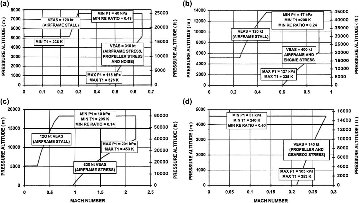
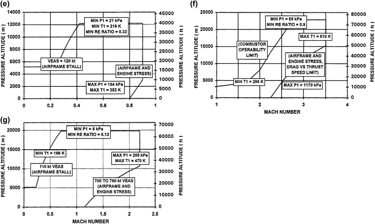
(e) Subsonic airbreathing missile, drone, or RPV. (f) Supersonic airbreathing missile. (g) Advanced military fighter. (Source: Rolls Royce.)
Notes: APUs have lower intake RAM recovery than propulsion engines.
Pressures shown are free stream, i.e., 100% RAM recovery.
To convert temperatures in K to R multiply by 1.8.
To convert temperatures in K to C subtract 273.15.
To convert temperatures in K to F multiply by 1.8 and subtract 459.67.
To convert pressures in kPa to psia multiply by 0.145038
To convert speeds in kt to km/h m/s miles/h ft/s multiply by 1.8520, 0.5144, 1.1508, 1.6878.
Maximum temperatures shown are for MIL STD 210 Hot day.
Minimum temperatures shown are for MIL STD 210 Cold day.
Minimum Reynolds’ Number ratios shown are for MIL STD 210 Hot day.
Unducted fans would have similar flight envelope to commercial turbofans.
“RPV”= Remotely Piloted Vehicle.
All numbers shown are indicative, for guidance only.
For each flight envelope the minimum and maximum free stream temperatures and pressures the engine would experience are shown, together with basic reasons for the shape of the envelope. Where auxiliary power units are employed the same free stream conditions are experienced as for the propulsion unit. The intake ram recovery is often lower, however, due both to placement at the rear of the fuselage and drag constraints on the intake design.
Free Stream Total Pressure and Temperature
The free stream total pressure (P0) is a function of both pressure altitude and flight Mach number. Free stream total temperature (T0) is a function also of ambient temperature and flight Mach number. Both inlet pressure and temperature are fundamental to engine performance. They are often used to refer engine parameters to ISA sea level static conditions, via quasi dimensionless parameter groups. To do this the following ratios are defined:
Definitions of Flight Speed
Traditionally aircraft speed has been measured using a pitot-static head located on a long tube projecting forward from the wing or fuselage nose. The difference between total and static pressure is used to evaluate velocity, which is shown on a visual display unit or gauge in the cockpit. The device is normally calibrated at sea level, which has given rise to a number of definitions of flight speed:
• Indicated air speed (VIAS) is the speed indicated in the cockpit based upon the above calibration.
• Calibrated air speed (VCAS) is approximately equal to VIAS with the only difference being a small adjustment to allow for aircraft disturbance of the static pressure field around the pitot-static probe.
• Equivalent air speed (VEAS) results from correcting VCAS for the lower ambient pressure at altitude versus that embedded in the probe calibration conducted at sea level, i.e., for a given Mach number the dynamic head is smaller at altitude. When at sea level VEAS is equal to VCAS.
• True air speed (VTAS) is the actual speed of the aircraft relative to the air. It is evaluated by multiplying VEAS by the square root of relative density as presented in Figure 19–4. This correction is due to the fact that the density of air at sea level is embedded in the probe calibration that provides VIAS. Both density and velocity make up dynamic pressure.
• Mach number (M) is the ratio of true air speed to the local speed of sound.
VEAS and VCAS are functions of pressure altitude and Mach number only. The difference between VEAS and VCAS is termed the scale altitude effect (SAE), and is independent of ambient temperature. Conversely, VTAS is a function of ambient temperature and Mach number, which is independent of pressure altitude.
To a pilot both Mach number and ground air speed are important. The former dictates critical aircraft aerodynamic conditions such as shock or stall, whereas the latter is vital for navigation. For gas turbine engineers Mach number is of paramount importance in determining inlet total conditions from ambient static. Often, however, when analyzing engine performance data from flight tests only VCAS or VEAS are available.
Properties and Charts for Dry Air, Combustion Products, and Other Working Fluids2
The properties of the working fluid in a gas turbine engine have a powerful impact upon its performance. It is essential that these gas properties are accounted rigorously in calculations, or that any inaccuracy due to simplifying assumptions is quantified and understood. This chapter describes at an engineering level the fundamental gas properties of concern, and their various interrelationships. It also provides a comprehensive database for use in calculations for:
Description of Fundamental Gas Properties
Equation of State for a Perfect Gas
A perfect gas adheres to Formula F19.1. All gases employed as the working fluid in gas turbine engines, except for water vapor, may be considered as perfect gases without compromising calculation accuracy. When the mass fraction of water vapor is less than 10%, which is usually the case when it results from the combination of ambient humidity and products of combustion, then for performance calculations the gas mixture may still be considered perfect. When water vapor content exceeds 10% the assumption of a perfect gas is no longer valid and for rigorous calculations steam tables must be employed in parallel, for that fraction of the mixture.
A physical description of a perfect gas is that its enthalpy is only a function of temperature and not pressure, as there are no intermolecular forces to absorb or release energy when density changes.
Molecular Weight and the Mole
The molecular weight for a pure gas is defined in the Periodic Table. For mixtures of gases, such as air, the molecular weight may be found by averaging the constituents on a molar (volumetric) basis. This is because a mole contains a fixed number of molecules, as described.
A mole is the quantity of a substance such that the mass is equal to the molecular weight in grams. For any perfect gas 1 mole occupies a volume of 22.4 liters at 0°C, 101.325 kPa. A mole contains the Avogadro’s number of molecules, 6.023 × 10²³.
Specific Heat at Constant Pressure (CP) and at Constant Volume (CV)
These are the amounts of energy required to raise the temperature of 1 kilogram of the gas by 1°C, at constant pressure and volume, respectively. For gas turbine engines, with a steady flow of gas (as opposed to piston engines where it is intermittent) only the specific heat at constant pressure, CP, is used directly. This is referred to hereafter simply as specific heat.
For the gases of interest specific heat is a function of only gas composition and static temperature. For performance calculations total temperature can normally be used up to Mach numbers of 0.4 with negligible loss in accuracy, since dynamic temperature remains a low proportion of the total.
Gas Constant (R)
The gas constant appears extensively in formulae relating pressure and temperature changes, and is numerically equal to the difference between CP and CV. The gas constant for an individual gas is the universal gas constant divided by the molecular weight, and has units of J/kg K. The universal gas constant has a value of 8314.3 J/mol K.
Ratio of Specific Heats, Gamma (γ) (Formulae F19.6–F19.8)
This is the ratio of the specific heat at constant pressure to that at constant volume. Again, it is a function of gas composition and static temperature, but total temperature may be used when the Mach number is less than 0.4. Gamma appears extensively in the “perfect gas” formulae relating pressure and temperature changes and component efficiencies.
Dynamic Viscosity (VIS) and Reynolds Number (RE) (Formulae F19.9)
Dynamic viscosity is used to calculate the Reynolds number, which reflects the ratio of momentum to viscous forces present in a fluid. The Reynolds number is used in many performance calculations, such as for disc windage, and has a second-order effect on component efficiencies. Dynamic viscosity is a measure of the viscous forces and is a function of gas composition and static temperature. As viscosity has only a second-order effect on an engine cycle, total temperature may be used up to a Mach number of 0.6. The effect of fuel air ratio (gas composition) is negligible for practical purposes.
The units of viscosity of N s/m2 are derived from N/(m/s)/m; force per unit gradient of velocity. Gas velocity varies in a direction perpendicular to the flow in the boundary layers on all gas washed surfaces.
Description of Key Thermodynamic Parameters
The key thermodynamic parameters most widely used in gas turbine performance calculations are described below. Their interrelationships are dependent upon the values of the fundamental gas properties described above.
Total or Stagnation Temperature (T) (Formula F19.10)
Total temperature is the temperature resulting from bringing a gas stream to rest with no work or heat transfer. Note that here “at rest” means relative to the engine, which may have a flight velocity relative to the Earth. The difference between the total and static temperatures at a given point is called the dynamic temperature. The ratio of total to static temperature is a function of only gamma and Mach number, as per Formula F19.10.
In general for gas turbine performance calculations total temperature is used through the engine, evaluated at engine entry from the ambient static temperature and any ram effect. At locations between engine components total temperature is a valid measure of energy changes. In addition, this aids comparison between predictions and test data, as it is only practical to measure total temperature. For most component design purposes, however, static conditions are also relevant, as for example the Mach number is often high (1.0 and greater) at entry to a compressor stator or turbine rotor blade.
Total temperature is constant for flow along ducts where there is no work or heat transfer, such as intake and exhaust systems. Total and static temperature diverge much less rapidly versus Mach number than do total and static pressure, as described below.
Total or Stagnation Pressure (P) (Formulae F19.11, F19.12, and F19.13)
Total pressure is that which would result from bringing a gas stream to rest without any work or heat transfer, and without any change in entropy. Total pressure is therefore an idealized property.
The difference between total and static pressure at a point is called either the dynamic pressure, dynamic head, or velocity head (Formulae F19.12 and F19.13). The term head relates back to hydraulic engineering. The ratio of total to static pressure, as for temperature, is a function of only gamma and Mach number. Most performance calculations are conducted using total pressure, that at engine inlet again resulting from ambient static plus intake ram recovery.
Total pressure is not constant for flow through ducts, being reduced by wall friction and changes in flow direction, which produce turbulent losses. Both these effects act on the dynamic head; the pressure loss in a duct of given geometry and inlet swirl angle is almost always a fixed number of inlet dynamic heads. For this reason for performance calculations both the total and static pressure must often be evaluated at entry to ducts. Again, for component design purposes both the total and static values are of interest.
Total and static pressure diverge much more rapidly versus Mach number than do total and static temperature. Calculation of pressure ratio from temperature ratio is far more sensitive to errors in the assumption of the mean gamma than the reverse calculation.
Specific Enthalpy (H) (Formulae F19.14, F19.15)
This is the energy per kilogram of gas relative to a stipulated zero datum. Changes in enthalpy, rather than absolute values, are important for gas turbine performance. Total or static enthalpy may be calculated, depending on which of the respective temperatures is used. Total enthalpy, like total temperature, is most common in performance calculations.
Specific Entropy (S)
Traditionally the property entropy has been shrouded in mystery, primarily due to being less tangible than the other properties discussed in this section. Entropy relates to other thermodynamic properties relevant to gas turbine performance, and thereby helps overcome these difficulties.
During compression or expansion the increase in entropy is a measure of the thermal energy lost to friction, which becomes unavailable as useful work.
Composition of Dry Air and Combustion Products
Dry Air
Dry air comprises the elements in Table 19–2.
TABLE 19–2
| By Mole or Volume (%) | By Mass (%) | |
| Nitrogen (N2) | 78.08 | 75.52 |
| Oxygen (O2) | 20.95 | 23.14 |
| Argon (Ar) | 0.93 | 1.28 |
| Carbon dioxide | 0.03 | 0.05 |
| Neon | 0.002 | 0.001 |
(Source: Rolls Royce.)
There are also trace amounts of helium, methane, krypton, hydrogen, nitrous oxide, and xenon. These are negligible for gas turbine performance purposes.
Combustion Products
When a hydrocarbon fuel is burned in air, combustion products change the composition significantly. Atmospheric oxygen is consumed to oxidize the hydrogen and carbon, creating water and carbon dioxide, respectively. The degree of change in air composition depends both on fuel air ratio and fuel chemistry. The fuel air ratio such that all the oxygen is consumed is termed stoichiometric.
Distilled liquid fuels such as kerosene or diesel each have relatively fixed chemistry. Properties of their combustion products can be evaluated versus fuel air ratio and temperature using unique formulae, with the fuel chemistry inbuilt. In contrast, the chemistry of natural gas varies considerably. All natural gases have a high proportion of light hydrocarbons, often with other gases such as nitrogen, carbon dioxide, or hydrogen. Because the composition of natural gas combustion products varies, along with the fuel chemistry, unique formulae for their gas properties do not exist, hence the calculation is more complex.
The Use of CP and Gamma, or Specific Enthalpy and Entropy, in Calculations
Either CP and gamma, or specific enthalpy and entropy, are used extensively in performance calculations. The manner of their use is described below in order of increasing accuracy and calculation complexity. This list covers all gas turbine components except for the combustor.
Constant, Standard Values for CP and Gamma
This normally uses the following approximations:
• Cold end gas properties: CP = 1004.7J/kg K, gamma = 1.4
• Hot end gas properties: CP = 1156.9J/kg K, gamma = 1.33
• Component performance: Formulae use values of CP and gamma as above
This is the least accurate method, giving errors of up to 5% in leading performance parameters. It should only be used in illustrative calculations for teaching purposes, or for crude “ballpark” estimates.
Values for CP and Gamma Based on Mean Temperature
For formulae using CP and gamma it is most accurate to base these values on the mean temperature within each component, i.e., the arithmetic mean of the inlet and exit values. It is less accurate to evaluate CP and gamma at inlet and exit, and then take a mean value for each.
For dry air and combustion products of kerosene or diesel the formulae given for CP as a function of temperature and fuel air ratio give accuracies of within 1.5% for leading performance parameters. The largest errors occur at the highest pressure ratios.
Specific Enthalpy and Entropy—Dry Air, and Diesel or Kerosene
For fully rigorous calculations changes in enthalpy and entropy across components must be accurately evaluated. This improves accuracy to be within 0.25% for leading parameters at all pressure ratios. Here polynomials of specific enthalpy and entropy are utilized, obtained by integration of the standard polynomials for specific heat. In these methods, a formula for specific heat is therefore still required.
The use of specific enthalpy and entropy for performance calculations is now almost mandatory for computer “library” routines in large companies.
Specific Enthalpy and Entropy—Natural Gas
For the combustion products of natural gas it is logical to use specific enthalpy and entropy only if CP is evaluated accurately.
Database for Fundamental and Thermodynamic Gas Properties
Molecular Weight and Gas Constant
Data for gases of interest are listed in Table 19–3.
TABLE 19–3
Molecular Weight and Gas Constants
| Molecular Weight | Gas Constant (J/kg K) | |
| Dry air | 28.964 | 287.05 |
| Oxygen | 31.999 | 259.83 |
| Water | 18.015 | 461.51 |
| Carbon dioxide | 44.010 | 188.92 |
| Nitrogen | 28.013 | 296.80 |
| Argon | 39.948 | 208.13 |
| Hydrogen | 2.016 | 4124.16 |
| Neon | 20.183 | 411.95 |
| Helium | 4.003 | 2077.02 |
Note: The universal gas constant is 8314.3 J/mol K.
(Source: Rolls Royce.)
Figure 19–10 shows the gas constant resulting from the combustion of leading fuel types in air plotted versus fuel air ratio. It is not possible to provide all encompassing data for natural gas due to the wide variety of blends that occur. For indicative purposes combustion of a sample natural gas has been used. The following are apparent:
• For kerosene, molecular weight and gas constant are not changed noticeably from the values for dry air up to stoichiometric fuel to air ratio.
• For diesel molecular weight and hence gas constant change minimally, in a linear fashion versus fuel to air ratio. For performance calculations there is negligible loss in accuracy by ignoring these small changes and using data for kerosene.
• For the sample natural gas molecular weight and gas constant vary linearly with fuel air ratio from the values for dry air to 27.975 and 297.15 J/kg K, respectively, at a fuel to air ratio of 0.05. A significant loss of accuracy will occur if this change is not accounted.
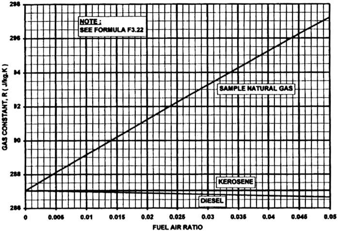
The effect of gas fuel is more powerful than that of liquid fuels, primarily due to the constituent hydrocarbons being lighter (i.e., containing less carbon and more hydrogen); this results in a higher proportion of water vapor after combustion, which has a significantly lower molecular weight than the other constituents.
Specific Heat and Gamma
Figures 19–11 and 19–12 present specific heat and gamma respectively for dry air and combustion products versus static temperature and fuel air ratio for kerosene or diesel fuels.
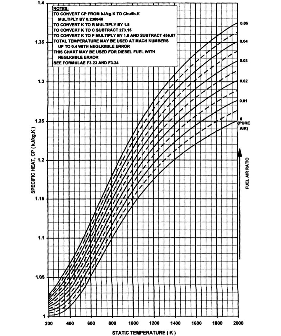
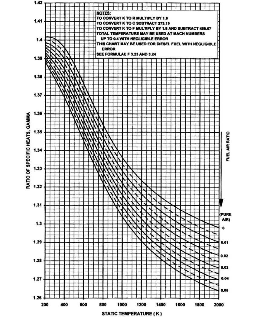
Figure 19–13 shows the ratio of specific heat following the combustion of the sample natural gas to that for kerosene, versus fuel to air ratio. This plot is sensibly independent of temperature. As stated earlier, specific heat is noticeably higher following the combustion of natural gas due to the higher resultant water content, which significantly impacts engine performance.
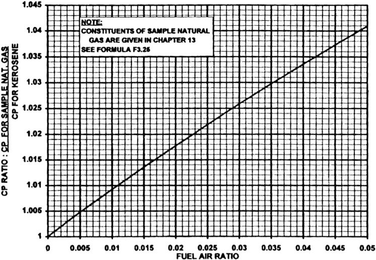
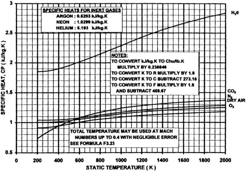
Figure 19–14 shows specific heat respectively versus temperature for the individual gases present in air and combustion products. The higher value for water vapor is immediately apparent. For inert gases such as helium, argon, and neon, specific heat and gamma do not change with temperature.
Temperature Entropy Diagram for Dry Air
Most heat engine cycles are taught at university level via schematic illustration on a temperature–entropy (T–S) diagram. This approach becomes laborious to extend to “real” engine effects such as internal bleeds and cooling flows, but remains a useful indication of the overall thermodynamics of a known engine cycle. Figure 19–15 presents an actual temperature–entropy diagram for dry air, complete with numbers, showing lines of constant pressure. Such a diagram is rare in the open literature.
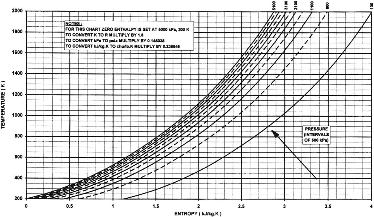
• Raising temperature at constant pressure (e.g., by adding heat in a combustor) raises entropy.
• Reducing temperature at constant pressure (e.g., by removing heat in an intercooler) lowers entropy.
• Compression from a lower to a higher constant pressure line (i.e., by adding work) produces minimum change in temperature (i.e., requires minimum energy input) if entropy does not increase. Isentropic compression is an idealized process.
• In reality entropy does increase during compression, hence extra energy must be provided, beyond the ideal work required for the pressure change. This extra energy is converted to heat.
• Expansion from a higher to a lower constant pressure line produces maximum change in temperature (i.e., produces maximum work) if entropy does not increase. Isentropic expansion is also an idealized process.
• In reality entropy does increase during expansion, hence less work output is obtained than the ideal work produced pressure change. This “lost” energy is retained as heat.
Entropy may be defined as thermal energy not available for doing work. In real compressors and turbines some energy goes into raising entropy, as some pressure is lost to real effects such as friction. The ideal work would be required or produced if entropy did not change, i.e., the process were isentropic. Isentropic efficiency is defined as the appropriate ratio of actual and ideal work, and is always less than 100%. (The term adiabatic efficiency is also commonly used, but is strictly incorrect. It only excludes heat transfer but not friction, and an isentropic process would have neither.)
Gas turbine cycles utilize the above processes, and rely on one other vital, fundamental thermodynamic effect:
Work input, approximately proportional to temperature rise, for a given compression ratio from low temperature is significantly lower than the work output from the same expansion ratio from higher temperature.
This is because on the T–S diagram lines of constant pressure diverge with increasing temperature and entropy.
This can be seen by considering a sample compression, heating, and expansion between two lines of constant pressure, using Figure 19–15. At an entropy value of 1.5 kJ/kg K the temperature rise required to go from 100 to 5100 kPa is 500 K. If fuel is now burned at this pressure level such that entropy increases to 2.75 kJ/kg K, and temperature to 1850 K, an expansion back to 100 kPa will achieve a temperature drop of around 1000 K. This clearly illustrates the rationale behind the Brayton cycle.
Schematic T–S Diagrams for Major Engine Cycles
Figures 19–16 through 19–21 show the key cycles of interest to gas turbine engineers.
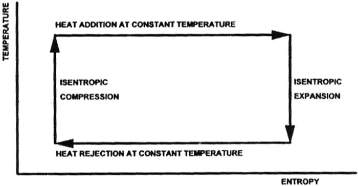
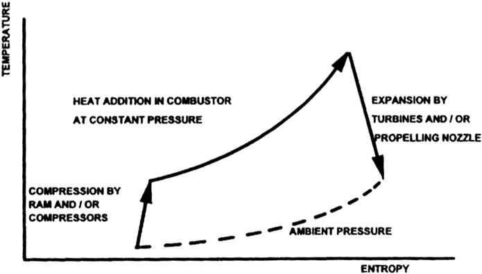
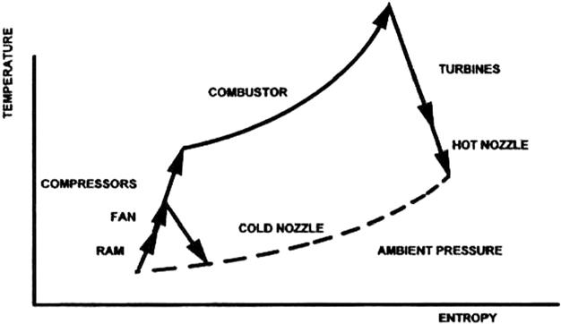
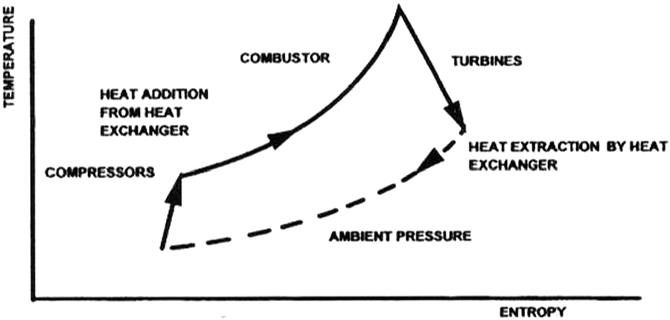
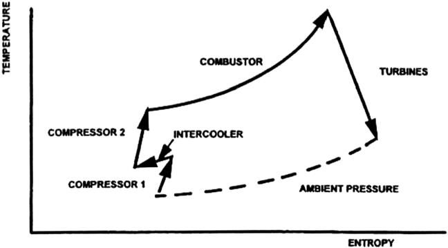
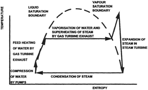
Figure 19–16 shows the Carnot cycle. This is the most efficient cycle theoretically possible between two temperature levels. Gas turbine engines necessarily do not use the Carnot cycle, as unlike steam cycles they cannot add or reject heat at constant temperature.
Figure 19–17 shows the Brayton cycle. This is the basic cycle utilized by all gas turbine engines where heat is input at constant pressure. The effect of component inefficiency is shown by the non-vertical compression and expansion lines, a further difference from the ideal Carnot cycle. The form of the Brayton cycle is modified for heat exchangers and bypass flows.
Figure 19–18 presents the cycle for a turbofan. The bypass stream only undergoes partial compression, and no heating before expansion back to ambient pressure.
Figure 19–19 shows a heat exchanged cycle. Waste heat from exhaust gases is used to heat air from compressor delivery prior to combustion, thereby reducing the required fuel flow.
Figure 19–20 presents an intercooled cycle, where heat is extracted downstream of an initial compressor. This reduces the work required to drive a second compressor, and thereby increases power output.
Figure 19–21 shows a Rankine cycle with superheat. This is used in combined-cycle applications, with the gas turbine exhaust gases providing heat to raise steam. Where heat is added at constant temperature during evaporation a close approximation to the Carnot cycle is achieved, the main deviation being the non-ideal component efficiencies.
Formulae
F19.1. Equation of state for perfect gas
F19.2. Specific heat at constant pressure (J/kg K) = fn(specific enthalpy (J/kg), static temperature (K))
F19.3. Specific heat at constant volume (J/kg K) = fn(specific internal energy (J/kg), static temperature (K))
F19.4. Gas constant (J/kg K) = fn(universal gas constant (J/kg K), molecular weight)
where the universal gas constant Runiversal = 8314.3 J/mol K.
F19.5. Gas constant (J/kg K) = fn(CP (J/kg K), CV (J/kg K))
F19.6. Gamma = fn(CP (J/kg K), CV (J/kg K))
F19.7. Gamma = fn(gas constant (J/kg K), CP (J/kg K))
F19.8. The gamma exponent (γ – 1)/γ = n(gas constant (J/kg K), CP (J/kg K))
F19.9. Dynamic viscosity of dry air (N s/m2) = fn(shear stress (N/m2), velocity gradient (m/s m), static temperature (K))
1. Fshear is the shear stress in the fluid.
2. V is the velocity in the direction of the shear stress.
3. dV/dy is the velocity gradient perpendicular to the shear stress.
F19.10. Total temperature (K) = fn(static temp (K), gas velocity (m/s), CP (J/kg K))
F19.11. Total pressure (kPa) = fn(total to static temperature ratio, gamma)
Note: This is the definition of total pressure.
F19.12. Dynamic head (kPa) = fn(total pressure
(kPa), static pressure (kPa))
F19.13. Dynamic head (kPa) = fn(density (kg/m3), velocity (m/s), Mach number)
For incompressible flow, such as that of liquids, it is sufficient to only use the first term—this is the well-known Bernoulli equation.
F19.14. Specific enthalpy (kJ/kg) = fn(temperature (K), CP (kJ/kg K))
H0 is an arbitrarily defined datum. The datum is unimportant in gas turbine performance as it is changes in enthalpy that are of interest.
F19.15. Change in enthalpy (kJ/kg) = fn(temperature (K), CP (kJ/kg K))
“Design Point” Engine Design, Definitions, and Terminology3
The Engine Design Point and Design Point Performance
For initial definition work, the operating condition where an engine will spend most time has been traditionally chosen as the engine design point. For an industrial unit this would normally be ISO base load, or for an aeroengine cruise at altitude on an ISA day. Alternatively some important high power condition may be chosen. Either way, at the design point the engine configuration, component design, and cycle parameters are optimized. The method used is the design point performance calculation. Each time input parameters are changed and this calculation procedure is repeated, the resulting change to the engine design requires a different engine geometry, at the fixed operating condition.
For the concept design phase described here the component design points are usually at the same operating condition as the engine design point. In a detailed design phase, however, this may not be true. For example, in the detailed design phase an aeroengine fan may be designed at the top of climb, the highest referred speed and flow, whereas the engine design point would be cruise. The term design point refers to the engine design point in the concept design phase, which is taken to be coincident with the component design points.
Design Point Performance Parameters, Definitions
Engine Performance Parameters
A number of key parameters that define overall engine performance are utilized to assess the suitability of a given engine design to the application, or compare several possible engine designs. These engine performance parameters are described as follows:
• Output power or nett thrust (PW, FN). The required output power or nett thrust is almost always the fundamental goal for the engine design. It is evaluated via the overall cycle calculation. The term effective or equivalent power is used for turboprops and turboshafts, where any residual thrust in the exhaust is converted to a power value and added to the shaft output power.
• Exhaust gas power. For a turboshaft engine core this is the output power that would be produced by a power turbine of 100% efficiency. It is of interest when engine cores are tested or supplied without their free power turbine, which may remain with the installation or be supplied by another collaborating company.
• Specific power or thrust (SPW, SFN). This is the amount of output power or thrust per unit of mass flow entering the engine. It provides a good first-order indication of the engine weight, frontal area, and volume. It is particularly important to maximize specific power or thrust in applications where engine weight or volume are crucial, or for aircraft that fly at high Mach numbers where the drag per unit frontal area is high. For turboprops and turboshafts and effective specific power may be evaluated, based on the effective power value.
• Specific fuel consumption (SFC). This is the mass of fuel burned per unit time per unit of output power or thrust. It is important to minimize SFC for applications where the weight and/or cost of the fuel is significant versus the penalties of doing so. When quoting SFC values it is imperative to state the calorific value of the fuel, and whether it is the higher or lower heating value, to ensure valid “back to back” comparisons. Again, for turboprops and turboshafts an effective SFC may be evaluated.
• Thermal efficiency for shaft power engines (ETATH). This is the engine power output divided by the rate of fuel energy input, usually expressed as a percentage. It is effectively the reciprocal of SFC, but is independent of fuel calorific value. However, when quoting thermal efficiencies it is still important to state whether the values are based upon the higher or lower fuel heating value. For combined-cycle applications the terms gross and nett thermal efficiency are used. Gross thermal efficiency does not deduct the power required to drive the steam plant auxiliaries, whereas nett values do.
• Thermal efficiency is usually quoted for industrial gas turbines, and SFC for aircraft turboshafts and turboprops. For marine and automotive gas turbines both terms are commonly used. This difference reflects the higher importance of fuel weight in aero applications, and the lower likely variation of fuel calorific values.
• Heat rate for shaft power cycles (HRATE). Heat rate is a parameter used only in the power generation industry, and is the rate of fuel energy input divided by the useful power output. Hence it is comparable to SFC but is independent of fuel calorific value. Again it is important to state whether higher or lower calorific value has been assumed in calculating fuel energy input, and for combined-cycle applications whether the values are gross or net.
• Exhaust temperature (T6). For engines used in combined cycle for industrial power generation, high exhaust temperature is vital in maximizing overall efficiency. For combined heat and power the optimum value depends on the relative demand of heat versus power. In both cases there is a limit to the allowable exhaust temperature due to mechanical integrity considerations in the steam plant.
• For military aircraft applications low exhaust gas temperature is important to reduce the infrared signature presented to heat seeking missiles.
• Exhaust mass flow (W6). For engines used in combined-cycle or combined heat and power applications the exhaust mass flow is important in indicating the heat available in the gas turbine exhaust, and hence the overall plant thermal efficiency.
For aircraft thrust engines there are a number of secondary performance parameters. These do not in themselves describe overall engine performance, but do help the engine designer understand the variation of the primary performance parameters across a number of designs. These parameters are as follows:
• Thermal efficiency. Thermal efficiency for aircraft thrust engines is defined as the rate of addition of kinetic energy to the air divided by the rate of fuel energy supplied, usually expressed as a percentage. The energy in the jet is proportional to the difference in the squares of jet and flight velocities. Generally thermal efficiency increases as pressure ratio and SOT increase together, as this results in a higher jet velocity for a given energy input.
• Propulsive efficiency (ETAPROP). Propulsive efficiency for aircraft thrust engines is defined as the useful propulsive power produced by the engine divided by the rate of kinetic energy addition to the air, again usually expressed as a percentage. The nett thrust is proportional to the difference in the jet and flight velocities. Since power is force times velocity, propulsive power is proportional to the flight speed times the difference in the jet and flight velocities.
• Propulsive efficiency is improved by low jet velocities, due to lower energy wastage as jet kinetic energy. This requires high-pressure ratio and low SOT. However, low jet velocities produce lower thrust output, hence to achieve high propulsive efficiency, as well as a required thrust, high engine mass flow must be coupled with low jet velocities. This leads to engines of low specific thrust, which are large and heavy. Turbofan engines are based upon this principle.
Thrust SFC is directly proportional to flight speed, and inversely proportional to both thermal and propulsive efficiencies. The dependency on the efficiencies is intuitively obvious. The choice of pressure ratio and SOT for minimum SFC is a compromise between maximizing propulsive and thermal efficiency.
The dependency of thrust SFC on flight speed arises because fuel flow relates to power with the thermal and propulsive efficiencies fixed, and propulsive power is directly proportional to flight speed for a given thrust.
Cycle Design Parameters
The fundamental thermodynamics of gas turbine cycles in relation to temperature entropy diagrams show that the changes in pressure and temperature that the working fluid experiences strongly affect the engine performance parameters. The degree of change of pressure and temperature are reflected via the following cycle design parameters.
Overall Pressure Ratio
This is total pressure at compressor delivery divided by that at the engine inlet.
Stator Outlet Temperature (SOT)
This is the temperature of the gas able to do work at entry to the first turbine rotor. Other terms are also used to reflect maximum temperatures in a cycle:
• Rotor inlet temperature (RIT): this term is sometimes used in North America, and means the same as SOT.
• Combustor outlet temperature (COT): this is the temperature at the first turbine nozzle guide vane leading edge.
• Turbine entry temperature (TET): this can have either of the above meanings.
The standard definition for SOT, used herein, is:
The fully mixed out temperature resulting from combustion delivery gas mixing with all cooling air that enters upstream of the first turbine rotor, and is able to do work due to having momentum comparable to the nozzle guide vane flow.
Hence, in this definition, nozzle guide vane or platform cooling air entering upstream of the throat, or trailing edge cooling air ejected with the same momentum and direction as the main flow, would be included. However, front disc face cooling airflow would not be considered in evaluating SOT since it will not do work in the turbine rotor. For most gas turbine engine types it is desirable to raise SOT to as high a level as possible within mechanical design constraints.
In addition for turbofan engines two further cycle design parameters occur due to the parallel gas paths.
Fan Pressure Ratio
This is the ratio of fan delivery total pressure to that at fan inlet, and is usually lower for the core stream than the bypass due to lower blade speed.
Bypass Ratio
This is the ratio of mass flow rate for the cold stream to that for the hot stream.
Component Performance Parameters
A plethora of parameters define component performance in terms of efficiency, flow capacity, pressure loss, etc. As the level of component performance parameters improves, at fixed values of cycle design parameters, then the design point engine performance parameters also improve.
Changes in component performance parameters have a secondary effect on the optimum values of engine cycle design parameters.
Mechanical Design Parameters
For a given performance design point to be practical the mechanical design parameters must be kept within the limits of the materials, manufacturing, and production technology available. These are mechanical design restraints in relation to gas turbine engines:
• Creep as a function of material type, metal temperatures, stress level, or AN2
• Oxidation as a function of material and coating type, and metal temperatures
• Cyclic life (low cycle fatigue) as a function of material type and metal temperatures
• Disc and blade tensile stress as a function of rim speed or AN2
• Casing rupture as a function of compressor delivery pressure
• Choke or stall flutter as a function of fan or compressor referred speed
• Vibration (high cycle fatigue) of rotating components as a function of rotational speed and excitation parameters such as upstream blade numbers and pressure levels
Life Parameters
The two major life parameters are:
1. Time between overhauls (TBO).
2. Cyclic life (also called low cycle fatigue life): this is the number of times the engine is started, accelerated to full power, and eventually shut down, between overhauls.
The TBO is governed mainly by creep and oxidation life, while cyclic life is dictated by thermal stress levels. Typical life requirements for the major gas turbine applications are as shown in Table 19–4.
TABLE 19–4
| Application | TBO (hours) | Cycles |
| Power generation—base load | 25,000–50,000 | 3000 |
| Power generation—standby/peak lopping | 25,000 | 10,000 |
| Gas and oil pumping | 25,000–100,000 | 5000–10,000 |
| Automotive—family saloon | 5000 | 10,000 |
| Automotive—truck | 10,000 | 5000–10,000 |
| Marine—military | 5000–20,000 | 2000–3000 |
| Marine—fast ferry | 5000–10,000 | 3000 |
| Aeroengine—civil | 15,000 | 3000 |
| Aeroengine—military fighter∗ | 25–3000 | 25–3000 |
∗There is a large difference between past achievements and future targets as the emphasis has moved from performance to cost of ownership.
(Source: Rolls Royce.)
Fuel Type
Kerosene is the standard aviation fuel while marine engines burn diesel and most industrial applications use natural gas. The highly distilled forms of diesel used make little difference to performance compared with kerosene, but natural gas gives performance improvements because of the higher resulting specific heat of the combustion products.
Design Point Diagrams
A design point diagram is created by plotting engine performance parameters versus the cycle parameters. To produce the diagram the design point calculations are repeated varying each cycle parameter in turn through the range of interest; every point is a different engine geometry. These diagrams are useful in the engine design process for selecting the optimum cycle parameters, or for comparing the performance of different gas turbine types. Initially design point diagrams are prepared using constant component performance parameter levels for all combinations of cycle parameters. Later in the engine design process different individual component performance levels are used for each combination of cycle parameters, based on aerothermal component design work.
Referred Parameters
The design point charts may be applied to any altitude if the referred form of specific power or thrust, SFC, etc. is used. In this way the datum values for the charts are adjusted. A change in flight Mach number does change engine matching, however, unless all nozzles are choked, and also changes ram drag. The charts are not directly adaptable to other flight Mach numbers.
Linearly Scaling Components and Engines
During the concept design process the scaling of existing components, or occasionally a complete engine, will be considered wherever possible. If viable this will significantly reduce program cost and development risk.
Design Point Exchange Rates
Design point exchange rates show the impact of a small change, typically 1%, in leading component performance levels on engine design point performance parameters. All other component efficiencies and cycle parameters are held constant as the parameter in question is varied. In practice this would require many other components to be redesigned to change flow sizes. Tables of design point exchange rates are extremely useful in the engine design process in highlighting the most sensitive component design areas, and should always be produced.
Synthesis exchange rates are quite different, and are utilized for off-design analysis, whereas the component in question is modified no other components are redesigned. All components move or rematch to a different non-dimensional operating point. In consequence component performance parameter levels change, as well as cycle parameters.
Open Shaft Power Cycles
With one exception all gas turbine engine configurations are open cycle. Air that enters the front of the engine is not recirculated, but is exhausted back into the atmosphere.
Simple Cycle
This is the basic shaft power cycle. First, air is compressed, and then it is heated by burning fuel in the combustor. Next, expansion through one or more turbines produces power in excess of that required to drive the compressors, which is available as output. Whether the engine is single spool or free power turbine is only reflected in a design point diagram by any small change in assessed overall turbine efficiency:
• Thermal efficiency and specific power generally increase with SOT. Though less convenient, combustor temperature rise is a better gauge of the cycle’s ability to deliver power. When this is low, excess power is low and the losses due to component inefficiencies dominate, reducing both thermal efficiency and specific power.
• The optimum pressure ratio for thermal efficiency increases with SOT, being 12:1 at 1100 K and rising to over 40:1 at 1800 K. The fact that there is an optimum is because as well as high combustion temperature rise, high thermal efficiency also requires low exhaust temperature to minimize energy wastage. Maximum thermal efficiency occurs at the minimum value of the ratio of combustor temperature rise to exhaust temperature, reflecting the ratio of heat input to heat wastage. Achieving this mainly requires low exhaust temperature, hence the optimum pressure ratios are relatively high. At too high a pressure ratio the low combustor temperature rise offsets the low exhaust temperature, which reduces thermal efficiency.
• The optimum pressure ratio for specific power also increases with SOT but is only around half that for thermal efficiency, being only 7:1 at 1100 K rising to 20:1 at 1800 K. Maximum specific power occurs at the maximum difference between the combustor temperature rise and the exhaust temperature, which reflects work output. Achieving this is less dominated by exhaust temperature and more by the need to reduce compressor work.
• For mechanical integrity the combustor entry temperature must be limited to between 850 and 950 K, depending on the technology level.
• If the engine is to be used in combined cycle or combined heat and power then, exhaust temperature must be limited to between 800 and 900 K, depending on the technology level of the heat recovery system.
Recuperated Cycle
This is as per the simple cycle except that a heat exchanger transfers some of the heat in the exhaust to the compressor delivery air. If the gas and air streams do not mix the heat exchanger is known as a recuperator; if they do mix, as with the automotive ceramic rotating matrix variety, it is known as a regenerator:
• Thermal efficiency and specific power generally increase with SOT.
• At optimum pressure ratios the thermal efficiency is around 10% better than that for the simple cycle, due to the heat recovery reducing the fuel requirement. This difference reduces as SOT increases as the corresponding simple cycle becomes more efficient.
• The optimum pressure ratio for thermal efficiency is comparatively low since the difference between the exhaust and compressor delivery temperature is high, hence more heat may be recovered. This is the dominant effect of pressure ratio.
• The optimum pressure ratio for specific power is 7.5:1 at 1100 K and 23:1 at 1800 K, and is independent of effectiveness. It is very similar to that for simple cycle, being only slightly reduced by the additional pressure losses in the recuperator.
• Effectiveness is one of the few component design parameters that has a strong effect upon the optimum pressure ratio for thermal efficiency. As it is increased, the optimum pressure ratio decreases, since increased heat recovery more than offsets a poor simple cycle efficiency.
• Combustor inlet temperature rises with falling pressure ratio for a given SOT. This is because of the reduced power requirement to drive the compressor, which reduces the temperature drop in the turbines.
• For mechanical integrity the recuperator and combustor entry temperatures must be limited to between 850 and 950 K, depending on the technology level.
Intercooled Cycle
In this configuration the temperature of the air is reduced part way through the compression process using a heat exchanger and an external medium such as water. This increases power output via reduced compressor work, which is directly proportional to compressor inlet temperature. Generally thermal efficiency reduces as more fuel is required to reach a given SOT:
• Thermal efficiency and specific power generally increase with SOT.
• Thermal efficiency is marginally worse than for the simple cycle below the optimum simple cycle pressure ratio and significantly better above it. This is driven by the relative magnitudes of the extra power output and the extra fuel flow required to raise the lower compressor delivery temperature to the given SOT.
• The optimum pressure ratio for thermal efficiency is 18:1 at 1100 K and over 40:1 at 1800 K. This is higher than for simple cycle, as the intercooler gives most benefit with a comparatively high-pressure ratio.
• As the intercooler position is moved, thermal efficiency peaks with it 30% through the compression ratio, such that the first compressor pressure ratio would be the overall value raised to an exponent of 0.30. (The design point diagrams are drawn for the intercooler placed 50% through the compression such that the compressors have equal pressure ratios.)
• Specific power is approximately 20–40% higher than for simple cycle due to the reduction in the power to drive the compressor stages after the intercooler. This drive power is directly proportional to compressor inlet temperature for a given pressure ratio.
• The optimum pressure ratio for specific power is 12:1 at 1100 K and over 40:1 at 1800 K. Again this is higher than for simple cycle, and for the same reason.
• As the intercooler position is moved, specific power peaks with the intercooler 50% through the compression ratio, such that the compressors would have equal pressure ratios. This corresponds to rejecting more heat than for the case of optimum thermal efficiency, and clearly requires more fuel energy input.
Intercooled and Recuperated Cycle
This is the combination of intercooling and recuperation. The thermal efficiency loss due to intercooling is offset by increased exhaust heat recovery due to the lower recuperator air-side entry temperature:
• Thermal efficiency and specific power generally increase with SOT.
• Thermal efficiency is around 20% higher than for simple cycle for a given SOT at the respective optimum pressure ratios, as in concert both the intercooler and recuperator reduce fuel consumption.
• The optimum pressure ratio for thermal efficiency is 7:1 at 1100 K and 20:1 at 1800 K. However, the cycle curves are flatter versus pressure ratio than for the other configurations above.
• Again, increasing recuperator effectiveness significantly reduces the optimum pressure ratio for thermal efficiency.
• Specific power is around 10% lower than for an intercooled only cycle due to the recuperator pressure losses, but still significantly higher than for simple cycle.
• The optimum pressure ratio for specific power is 13:1 at 1100 K and over 30:1 at 1800 K. Again, the cycle curves are flatter versus pressure ratio than for the other configurations above.
• For mechanical integrity the recuperator and combustor entry temperatures must be limited to between 850 and 950 K, depending on the technology level.
• As the intercooler position is moved, thermal efficiency peaks with it 40% through the pressure rise, and specific power peaks with it at 50%.
Combined Cycle
This is where a steam (Rankine) cycle also generates power, using exhaust heat from a simple cycle gas turbine. In addition, supplementary firing may be employed whereby a separate boiler supplements the gas turbine heat output when necessary. The curves are for a triple pressure reheated steam plant:
• Thermal efficiency and specific power generally increase with SOT.
• Thermal efficiency exceeds that of all other configurations by around 20–30%.
• The optimum pressure ratio for thermal efficiency is 4:1 at 1100 K and around 21:1 at 1800 K. These values are lower than for simple cycle, as here increasing pressure ratio at a given SOT reduces the exhaust heat available for the steam cycle, reducing its efficiency. At the highest SOT levels the thermal efficiency curves are flatter versus pressure ratio than for all other configurations above; the steam cycle trends offset those of the gas turbine, benefiting from the higher exhaust temperature when gas turbine efficiency falls.
• As a rule of thumb, the pressure ratio that gives the best combined-cycle thermal efficiency, while retaining an acceptable gas turbine exit temperature, is the optimum value for simple cycle specific power.
• The optimum pressure ratio for specific power is less than 4:1 at 1100 K and 7:1 at 1800 K. These values are even lower than those for simple cycle due to the effect of high gas turbine exit temperature on steam plant power.
• The exhaust temperature limits of 800–900 K discussed for simple cycle engines must be considered here.
Combined Heat and Power
This configuration differs from those above in that the engine exhaust heat is also utilized in the application, either directly in an industrial process or to raise steam for space heating. A varying amount of exhaust heat may be utilized or wasted, hence heat to power ratio is an important parameter in cycle comparisons. Again, supplementary firing may be employed:
• Thermal efficiency increases with SOT.
• Thermal efficiency increases almost linearly with heat to power ratio, as would be expected.
• Increasing pressure ratio increases thermal efficiency, though with diminishing returns above a value of 12:1. This reflects the corresponding simple cycle trends.
• Relatively high exhaust temperature, as given by a high specific power gas turbine, is often beneficial as high-grade heat is more useful for a variety of processes. The exhaust temperature limits of 800–900 K discussed for simple cycle engines must be considered here, however.
Closed Cycles
Here the working fluid is recirculated through the cycle. Heat exchangers are employed in place of the intake/exhaust and combustion processes, passing heat to and from external media. Maximum temperatures are limited by heat exchanger mechanical integrity, and unlike for open cycles, compressor entry pressure may be controlled to vary power level. Applications involve energy sources unsuited to direct combustion within a gas turbine engine, such as nuclear reactors or alternative fuels. The working fluid is normally helium, due to its high specific heat:
• Thermal efficiency and “power ratio” generally increase with SOT.
• The “power ratio” as presented is specific power multiplied by the ratio of the density of helium at the inlet temperature and pressure to that of air at ISO conditions. This reflects the impact on the required engine size.
• The optimum pressure ratio for thermal efficiency is around 4:1.
• Reducing inlet temperature raises thermal efficiency and power ratio, via increased non-dimensional SOT, i.e., SOT/T1.
• Raising inlet pressure increases power ratio, via increased fluid density.
• The optimum pressure ratio for power ratio is around 6:1.
• Practical SOT levels are low, due to heat exchanger integrity limits.
Aircraft Engine Shaft Power Cycles
Here a simple cycle configuration produces shaft power, along with a residual exhaust thrust. SFC is plotted rather than thermal efficiency:
• SFC and specific power generally improve with SOT.
• At ISA SLS the optimum pressure ratio for SFC is 12:1 at 1100 K SOT and over 30:1 at 1700 K. At the typical turboprop cruise flight condition of 6000 m 0.5 M it is 17:1 at 1100 K SOT, and over 30:1 at 1700 K. The small increase in optimum pressure ratio is due to the increased cycle temperature ratio at the cooler inlet conditions at altitude, despite the change in matching produced by the flight Mach number.
• At both conditions the optimum pressure ratio for specific power is around 7:1 at 1100 K SOT and 19:1 at 1700 K.
Aircraft Engine Thrust Cycles
Turbojets
Here a simple cycle configuration produces thrust via high exhaust gas velocities.
Turbofans
Here air from the first compressor of what is otherwise a turbojet engine bypasses the remaining compressor and turbine stages. This air produces thrust directly, additional to that from the hot exhaust gases.
Ramjets
Here fuel is burned in air compressed solely by the intake ram effect; there is no turbomachinery. Engine performance parameters are therefore a function only of SOT and flight Mach number.
The Engine Concept Design Process
This section presents a simplified overview of the complex concept design process. To lead an engine concept design effectively requires a full understanding of gas turbine performance and all the associated design processes and their interrelationship. Equally, others involved in the process must have some knowledge of performance if they are to contribute to it beyond their own subject areas.
Statement of Requirements
A statement of requirements or specification for a new engine may be presented by a customer organization, or may be specified within the cycle designer’s company to meet a perceived market need. Realism is required in terms of technical challenge as well as potential development and unit production costs. The document must not just reflect what “Marketing” or “the Customer” desires but also what “Engineering” can achieve. It should be written jointly.
With respect to performance the statement of requirements must contain a minimum of:
• Performance targets both at design point and other key operating conditions. The relationship to average or minimum engine and in service deterioration must also be specified, as well as future growth potential.
• Full definition of operating conditions for the above, and also the entire operational envelope, including ambient temperature, pressure or pressure altitude, humidity, flight Mach number, and installation losses.
• The starting envelope, as well as starting and above idle transient response times.
• Fuel type and emissions requirements.
• Engine diameter, length, and weight.
• Time between overhauls and cyclic life.
• Design and development program duration and cost, as well as unit production cost.
“First Cut” Design Points
Generic design point diagrams will show what engine configurations, together with the levels of cycle parameters, are likely to meet the statement of requirements. Next, initial component performance targets are set. For the narrow range of cycle parameters of interest, refined design point diagrams are then produced. Usually component efficiency variation with engine cycle parameters is unknown at this stage. As far as possible the cycle designer takes account of mechanical design limits such as temperature levels and considers the use of existing or scaled components.
From these design point diagrams a first cut design point for each engine configuration under consideration is formally issued to component designers. An example of multiple configurations is that both simple cycle and recuperated engines may be competitive for a shaft power application.
For clarity all design points should have an identifying version number, as many more updates will follow in what is a highly iterative design process.
“First Cut” Aero-Thermal Component Design
The component specialists now reassess the component performance inputs assumed in the design points, and perform initial component sizing. Their analysis uses component design computer codes and empirical data. Mechanical design parameters are monitored and where there is doubt regarding limits mechanical technologists must be consulted.
Proper choice of rotational speed is crucial. It is key to achieving the target compressor and turbine efficiency levels as well as number of stages and diameter, and the compressor and turbine designers must agree upon it. The practicality or otherwise of using the number of spools that the cycle designer had in mind when setting the initial design points will soon be apparent, and weight and cost implications will become clear.
Component performance levels are now bid back to the performance engineer for each design point.
Design Point Calculations and Aero-Thermal Component Design Iterations
By repeating the design point calculations using the new bid component performance levels the concept design team can decide which engine configuration is the most suitable. If a bid is changed even for only one component, it will change the design point requirements for all others.
The process is repeated a number of times for the chosen configuration so that a number of cycle parameter combinations, each with specific component performance levels, can be compared.
Engine Layout
It is important to commence engine layout drawings as early as possible to highlight potential difficulties. For example, for a turbofan there would normally be a rigid engine diameter constraint. The core diameter required by the compressor and turbine designs, combined with the bypass duct annulus area to keep Mach number to a level where pressure loss is acceptable, may exceed this limit. In this instance the cycle designer may have to reduce bypass ratio, or the component designers increase rotational speed.
Off-Design Performance
Once a good candidate design point is emerging from the above iterations the cycle designer must then freeze the engine geometry and issue off-design performance. This should cover other key operating points as well as all corners of the operational envelope. Often at this juncture the component designers will not have created off-design maps for the “frozen” component designs so maps from existing components of similar design must be used, with factors and deltas applied to align them to the design point. The performance engineer must decide how the engine will be controlled for key ratings before running the off-design cases.
It is good practice at this stage for the performance engineer to highlight the operational cases where the maximum and minimum value of all key parameters occur, and any margins that need to be applied for say operating temperatures for a minimum engine.
Performance, Aero-Thermal, and Mechanical Design Investigation
The off-design performance data must be examined in detail by all parties. The cycle designer must check whether the engine design meets other performance requirements besides that at the design point. The aero-thermal and mechanical component designers must ensure that the components are satisfactory throughout the operational envelope with respect to component performance levels, stress, and vibration.
Basic Starting and above Idle Transient Performance Assessment
Engine operability is assessed by ensuring that surge and weak extinction margins are commensurate with the required accel, decel, and start times. A judgment is made with respect to the need for variable stator vanes or blow off valves (BOVs); these also impact compressor design, unless the BOVs are at compressor delivery, and may be inherited anyway if an existing compressor design is utilized. Unless there are unusual or severe requirements, modeling of transient performance or starting would not normally be conducted in the concept design phase. However, when such requirements are present or if a novel engine configuration is employed, then transient performance modeling is essential as transient considerations can significantly impact the fundamental engine design in terms of cycle, number of spools, etc.
Iterations
A number of iterations through the whole process concludes the concept design phase. The resulting engine design is then compared with the statement of requirements and a judgment made as to whether to proceed into a detailed design and development program.
Margins Required When Specifying Target Performance Levels
It is important that no ambiguities are present when performance targets for an engine design are specified, and that certain less obvious issues are not forgotten; some of the latter are outlined below.
Minimum Engine
Owing to manufacture and build tolerances there will be significant engine-to-engine variation in production. Usually the engine designers deal with average engine data, that is, the average performance of all production engines. However, if the customer has been guaranteed a given performance level then even the minimum engine must achieve this standard. Hence a design margin must be built into the average engine performance targets. The shortfall in power or thrust and SFC of a minimum engine in a production run will be 1–3% versus the average engine if run at constant temperature, depending on build quality and engine complexity. If the customer has been guaranteed levels of power or thrust then this minimum engine will run up to 20 K hotter than an average engine to achieve power or thrust. This must be allowed for in the mechanical design.
Design and Development Program Shortfall
At the outset of a program the risk of component performance levels falling short of the values used in any preliminary design point analysis must be assessed. Ideally some engine performance risk analysis should be employed to quantify the potential shortfall versus confidence level. Suitable margins should then be applied to the performance target levels.
However, at the outset of a program this level of risk analysis may not be commensurate with time or resource constraints and the available component performance database. In this instance judgment must be used. The level of the margins should reflect the confidence of component performance levels employed in any preliminary analysis. Each case must be considered individually, but typical margins are presented in Table 19–5 for three confidence levels that the components will meet their design targets.
TABLE 19–5
Typical Performance Margins, by Confidence Level
| High | Medium | Low | |
| Power or thrust SFC |
+2.5% –2% |
+5% –4% |
+7.5% –6% |
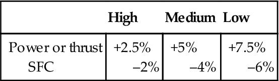
(Source: Rolls Royce.)
When in competitive tender for an engine application the luxury of SFC margins may not be allowed due to commercial constraints. However, for shaft power engines building in power margin is often practical by sizing the engine larger. In this instance, should the component performance levels employed in the preliminary analysis be achieved then almost invariably the customer will accept the extra power. In aircraft applications it may be more difficult to provide margin for thrust due to tight restrictions on weight and frontal area.
Growth Potential
Almost any engine must be capable of adaptation to higher power or thrust levels. In aircraft applications the airframe usually requires it, intentionally or otherwise. In addition, addressing a wider market with development costs spread over a family of engines is attractive economically. Examples for turbofans include the Rolls Royce RB211/Trent family (thrust growth of 180 to 400+ kN in 25 years), the Rolls Royce civil and military Spey family, and the General Electric CF6 range. Margin is required on levels of temperature and speed, and there must be a practical route to increasing engine mass flow.
Engine Deterioration
At the concept design stage it is unusual to specify performance requirements after deterioration over a number of hours in service. However, if this is the case then a margin must be allowed for from the outset. The amount required depends on whether in service the engine is governed to fixed levels of temperature, speed or thrust/power. Depending on engine complexity typical margins at 10,000 hours, expressed at constant SOT, are: +3 to +6% SFC; –5 to –15% power.
Performance degradation is usually exponential with time, and after 10,000 hours there is minimal further deterioration. Practices vary regarding the accounting or not of running in effects caused by initial seal cutting as part of deterioration. The aim of running in is to improve performance levels by ensuring a gentle first contact on key seals, which removes less material than would a first in-service rub.
One further effect is compressor fouling where accretion of airborne particles on aerofoil surfaces reduces flow and efficiency, raising engine temperature levels. This applies mainly to ground based engines and is recoverable via compressor washing, for which appropriate fluid injection nozzles must be provided. The temperature increase depends entirely on site location, filter effectiveness, and washing frequency.
Installation Losses
Usually performance targets are stipulated as uninstalled, with the engine performance quoted from the engine intake flange to the engine exhaust or propelling nozzle flange. If the performance targets are installed then the magnitude of all installation effects must be stated, as follows:
• Plant or airframe intake pressure loss
• Plant exhaust or airframe jet pipe pressure loss
• Customer auxiliary power offtake (gas turbine accessory power requirements should be accounted even for uninstalled performance)
• Whether shaft power output and thermal efficiency are at turbine, gearbox, or alternator output
Two case histories and one Mach number-altitude chart follow. Although the cases involve aircraft engine design, the principles are applicable to all gas turbines. The cases were written in 1972 and 1988, respectively, but they still draw interest today. Because the 1972 case is now hard to access, it is reprinted almost entirely.
Case Study 1: Prediction Effects of Mass-Transfer Cooling on the Blade-Row Efficiency of Turbine Airfoils4
Two analytical models for calculating the effect of injected coolant on cascade efficiency are presented. Both methods assume that the performance losses that accompany coolant injection are due wholly to the mixing of coolant and mainstream gases and may be superimposed on the basic boundary layer loss. One model employs the “influence coefficient” method, assuming that the differential form of the one-dimensional equation for compressible flow with injection may be applied to finite injection rates. This method, although approximate, does agree well with more exact calculations using one-dimensional constant static pressure mixing. The approximation also reveals the significant mixing loss parameters in a relatively simple form, showing that coolant injection effects are primarily dependent on mainstream Mach number, coolant fraction, coolant injection angle, and the ratios of coolant-to-mainstream total temperature and velocity. The second analytical model, primarily suited for numerical computation, employs the concept of one-dimensional mixing layers to calculate losses due to surface injection (film- or transpiration-cooling) but employs a two-dimensional solution for the flow downstream of the trailing edge in order to include the effects of airfoil boundary layers and trailing-edge coolant bleed. The numerical method has been applied to several stator-cooling configurations and good agreement with available data is obtained.
cp = Specific heat at constant pressure
s = Height of trailing-edge coolant jet when expanded to pressure P1
δ∗ = Total boundary layer displacement thickness at the trailing edge based on average freestream (Station 1) conditions
θ = Total momentum thickness at the trailing edge based on average mainstream (Station 1) conditions
η = Cascade thermodynamic efficiency
ξ = Ratio of coolant-to-mainstream mass flowrates
ϕc = Angle of coolant injection measured from local mainstream direction
1 = Average mainstream condition at the trailing-edge plane
2 = Fully-mixed equilibrium downstream state
f = Local condition downstream of injection
The increasing use of mass-transfer cooling in turbines has allowed significant increases in turbine inlet temperatures and overall engine performance. The problem of predicting the aerodynamic effects of injecting coolant air has grown in importance as mass-transfer cooling has increased in both extent of application and amount of cooling air employed. The rising costs of experimental testing have encouraged the development of analytical methods to predict the effects on blade-row performance of film-, transpiration-cooling, and the introduction of spent cooling air by methods such as airfoil trailing-edge bleed. The present case examines the purely aerodynamic loss, often called the “mixing loss,” due to coolant injection within a turbine airfoil blade row and its subsequent mixing with the mainstream flow. The general methods developed, however, may be applied to any portion of the turbine where coolant is injected.
Consider the turbine airfoil blade row of Figure 19–22, which represents a rotor or stator employing mass-transfer cooling. The thermodynamic efficiency for the cascade shown is defined as
(19.1)
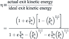 (19.1)
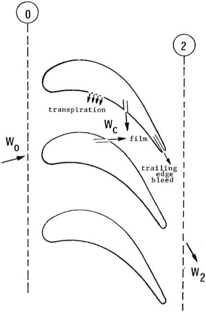
where Equation 19.1 is written for like, perfect gases and assumes that the ideal available kinetic energy of the exit flow is equal to the sum of the ideal kinetic energies of the coolant and inlet flows when expanded isentropically (without mixing) to the exit static pressure. For the particular case where ![]() , the efficiency expression reduces to the classical cascade efficiency,
, the efficiency expression reduces to the classical cascade efficiency,
(19.2)
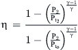 (19.2)
In engine applications ![]() is an external variable, usually dictated by the cycle coolant air availability, thus the airfoil cascade efficiency is determined by the average exit total pressure
is an external variable, usually dictated by the cycle coolant air availability, thus the airfoil cascade efficiency is determined by the average exit total pressure ![]() for a fixed coolant supply pressure. The prediction of cooled blade-row efficiency is thus equivalent to predicting the total pressure change
for a fixed coolant supply pressure. The prediction of cooled blade-row efficiency is thus equivalent to predicting the total pressure change ![]() caused by viscous effects, trailing-edge blockage, and coolant-primary flow mixing. The methods of this case are based on the assumption that these losses are additive and may be determined independently. This implies that the injected coolant mixes with the mainstream flow rather than remaining entrained in the boundary layer. Although the true situation is undoubtedly something between the two extremes of complete entrainment and complete mixing, there does exist experimental evidence to substantiate the present simple model.
caused by viscous effects, trailing-edge blockage, and coolant-primary flow mixing. The methods of this case are based on the assumption that these losses are additive and may be determined independently. This implies that the injected coolant mixes with the mainstream flow rather than remaining entrained in the boundary layer. Although the true situation is undoubtedly something between the two extremes of complete entrainment and complete mixing, there does exist experimental evidence to substantiate the present simple model.
One-Dimensional Methods
The simplest model for coolant-mainstream mixing is the one-dimensional slot shown in Figure 19–23. This may be viewed as an appropriate idealization of a single row of film-cooling holes or, if the imagination is willing, an “average” of a complex cooling geometry. Two solutions are readily obtained for the one-dimensional case.
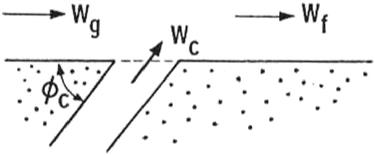
Constant Static Pressure Mixing
If the upper boundary of the flow shown in Figure 19–23 is assumed to be flexible, then coolant and mainstream flows may be mixed under the assumption of a constant static pressure. Applying the equations of continuity, streamwise momentum, energy, and assuming thermally and calorically perfect gases for both mainstream and coolant, the result
(19.3)
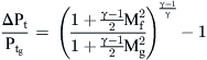 (19.3)
(19.4)
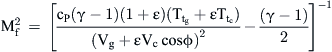 (19.4)
is obtained.
A Linear Approximation
The one-dimensional mixing of Figure 19–23 may also be approximated by adopting the “influence coefficient” method of Shapiro in the following manner.
For the compressible flow of a perfect gas having constant external and frictional forces, the differential variation of total pressure may be expressed as
with partial derivatives of
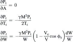
as obtained from the derivation by Shapiro. Rearranging gives
(19.5)
which assumes that the injected fluid enters the mainstream at the local static pressure. Exact solution of Equation 19.5 requires integration of the functions, but, assuming that relatively small variations of Tt and W occur, the differentials may be considered Δ’s. The term “linear approximation” is thus derived from the fact that the equation is thus linear in the independent variables dTt/Tt and dW/W. The term dTt/Tt may be simplified by assuming equal mainstream and coolant specific heats and writing the energy equation for a perfect gas in differential form as
which, when expanded and second-order terms are dropped, becomes
Since dW/W = ξ, Equation 19.5 may then be written in the more convenient form
(19.6)
A further simplification results when ![]() , in which
, in which
since γc = γg = γ has been assumed.
The linear approximation method is valuable, not merely because it allows rapid hand calculation, but also since it reveals the primary mixing-loss parameters in their simplest form. This is seen by comparing Equations 19.3 and 19.4 with Equation 19.6. The latter relationship shows that gas properties affect the mixing result only weakly through the specific heat ratio, while mainstream Mach number and coolant fraction are far more significant, as are the coolant-mainstream temperature ratio, velocity ratio, and the coolant injection angle. As would be expected from a one-dimensional analysis, the losses predicted for injection normal to the mainstream flow (ϕc = 90°) are independent of coolant velocity since the streamwise component of coolant momentum is zero for all coolant velocities.
Figures 19–24 and 19–25 present a comparison of calculated losses using both of the one-dimensional methods. A constant coolant area for each temperature ratio has been chosen so that coolant and mainstream total pressures are equal at a coolant mass fraction ξ = .03. Coolant velocity for high coolant pressures was limited to the sonic value for these calculations. Aside from showing the close agreement of the linear approximation with constant static pressure mixing, the effects of total temperature ratio and coolant injection angle are quite apparent.
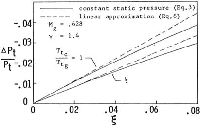
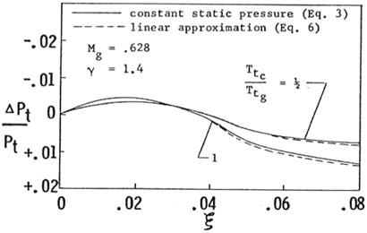
The close agreement of the two calculation methods is not surprising since they are, of course, identical in the limit of zero coolant addition. Figure 19–26 presents the linear approximation in terms of a dimensionless loss parameter in order to show the effects of temperature ratio and coolant injection angle for the ideal case in which coolant and mainstream gases are identical in composition, have equal total pressures, but differ in total temperature. Figure 19–26 is merely a graphic portrayal of the bracketed term in Equation 19.6. The result shows that not only do losses decrease with decreasing angle of injection, but it also reveals that as injection angle decreases, the effect of coolant-to-mainstream temperature ratio becomes less pronounced for higher temperature ratios and more evident for lower ratios. As coolant total temperature approaches extremely low values, the intuition that injection angle becomes less important is confirmed. For total temperature ratios in the general vicinity of ½, however, the effect of coolant injection angle is quite significant.
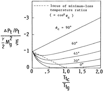
 ) [19-1].
It is also interesting to note that the one-dimensional methods discussed above are in close agreement with one-dimensional constant area mixing methods, which are far more difficult to apply, particularly for transonic Mach numbers.
The TOTLOS Method
The one-dimensional methods discussed above are based on the concept of coolant injection at a single location into a uniform mainstream. A more practical problem is that posed by complex cooling geometries in which injection occurs at a variety of locations having differing mainstream and coolant conditions. It is possible to apply the one-dimensional techniques by assuming coolant and mainstream parameters which are “typical” of the lumped cooling system, but the method of selecting the average parameters for such a simplification is not fore-known. The following method, called the TOTLOS method, allows the calculation of the total blade-row ΔPt due to viscous boundary layers, trailing-edge blockage, and coolant injection. The method, as with the one-dimensional ones just discussed, is based on the assumption that losses due to coolant-mainstream mixing may be superimposed on those due to boundary layers and other causes unrelated to cooling per se, such as airfoil base pressure drag and endwall losses.
Total pressure loss due to film or transpiration-cooling of the airfoil surface is found by applying the one-dimensional constant static pressure mixing method within a “mixing layer” over each surface, allowing coolant and mainstream flow to be mixed at successive “nodes” along the surface. These nodes may correspond to either rows of injection holes or arbitrary subdivisions of a porous region. The local static pressure of each node is equal to that on the airfoil surface at that particular station. As shown in Figure 19–27, the unaffected mainstream flow is then mixed with the contents of both surface-mixing layers (again using the one-dimensional constant static pressure mixing method) at a static pressure equal to the average mainstream value in the trailing edge plane (P1).
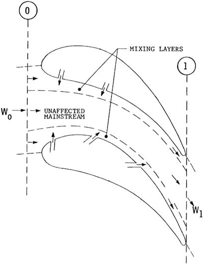
No theoretical basis for selecting the thickness of the mixing layers has been formulated to date, but numerical computations using the TOTLOS method show repeatedly that the final result is not significantly dependent on this parameter. As more experience is gained using the method as a comparison with experimental data, a dependence of mixing-layer size on other parameters may be discerned. Good candidates for such parameters would be cooling geometry, airfoil pressure distribution, mainstream turbulence, etc. For the present calculations, each mixing layer height at Station 0 has been arbitrarily set at 5% of blade-row pitch, and variation of this initial height from 3–30% of inlet pitch shows little effect on the final calculated loss.
The inclusion of viscous losses, trailing-edge blockage effects, and the effect of coolant injection from the trailing edge are accomplished using the two-dimensional model shown in Figure 19–28. The method used is based directly on that of Stewart, with some modification to include a coolant jet in the airfoil base. The desired result of the two-dimensional calculation between Stations 1 and 2 is the fully-mixed, uniform downstream state, particularly the total pressure and flow direction. The equations of continuity, tangential momentum, and axial momentum for the control volume shown are written as
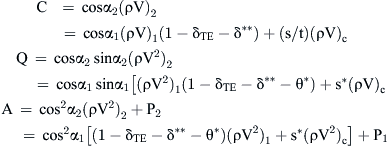
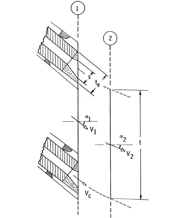
By introducing the energy and state equations, the system may be solved. The solution for the case of a perfect gas is a direct one, obtaining the downstream density as
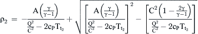
from which the complete flow condition at Station 2 may then be found using standard relationships.
Two required inputs for the inclusion of boundary layer losses in the final result are the displacement and momentum thicknesses at the trailing edge. The program of McDonel has been adopted for this purpose, but any comparable method could be used. The TOTLOS calculation scheme can become quite laborious if more than a few coolant-injection locations are specified, thus the method has been programmed for numerical computations, allowing the inclusion of real gas properties. Cooling geometries having up to 70 injection locations have been analyzed using the programmed version.
The TOTLOS calculation method has been applied to a series of cooled stator designs tested by The Lewis Research Center of NASA. Figures 19–29 through 19–31 present the variation of stator thermodynamic efficiency, both measured and predicted, for the three vane cooling configurations tested. These designs included film-cooling through holes drilled normal to the surface, transpiration-cooling employing porous wire-mesh surface segments, and trailing-edge injection through rectangular slots. The film- and transpiration-cooled designs incorporated coolant injection over the entire vane surface and all data were obtained in an annular stator at a coolant-to-mainstream total temperature ratio of 1.
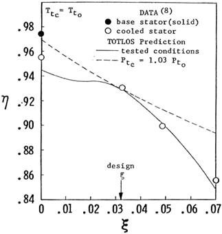
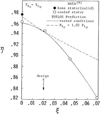
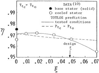
Since the TOTLOS method is two-dimensional, a “pitch-line” analysis at a nominal cascade pressure ratio of 1.5 was used to calculate the predicted stator efficiencies shown here. The calculations were carried out for each vane design for two distinctly different cases. One case, shown as the solid line in each figure, was for the tested conditions, i.e., coolant flow variation was achieved by varying the coolant supply pressure. This case obviously allows recirculation of mainstream flow within the vane coolant cavity for the film- and transpiration-cooled vanes at coolant total pressures below the stator inlet value.
To calculate a “net” coolant injection distribution over the surface in this range, the surface pressure distribution and the known coolant fraction were employed in an iterative solution to find the coolant supply pressure and the distribution of inflow or outflow over the vane surface. Once this surface flow distribution was found, the mainstream flow into the vane was neglected and only surface outflow was used in the loss calculation.
A second case, calculated for each vane design and shown as a dashed line in each figure, was the “design” case in which the coolant supply pressure was held constant at the design value, approximately equal to the inlet total pressure. The predicted efficiencies agree well with the data for coolant pressures equal to or above the design value, the region in which coolant flow distribution could be most accurately predicted. The large differences between efficiencies calculated for the “tested conditions” case and the “design” case at large coolant flows is due primarily to the fact that the ideal available kinetic energy of the coolant is charged to the stator at a total pressure considerably greater than inlet total pressure. As would be expected, trailing-edge coolant injection causes far less loss of efficiency than either normally-injected film- or transpiration-cooling for both the “test conditions” and “design” cases.
In summary, the effects of coolant injection on the flow through an airfoil cascade are admittedly complex and require analyses far more sophisticated than those given here if a detailed description of the resultant flowfield is desired. To the turbine designer, however, the methods presented here allow a relatively rapid determination of the effect of coolant injection on blade-row efficiency by predicting the state of the fully-mixed exit flow, a quantity of great interest to the engineer. Comparisons of predicted efficiency variations with data, such as those presented here, have shown the methods to be reliable and consistent. While their most useful application is in the evaluation of the aerodynamic performance of various cooling designs, reducing the amount of expensive testing required, the one-dimensional model also reveals the relative roles of mainstream Mach number, coolant-to-mainstream temperature and velocity ratios, and coolant injection angle in the generation of observed losses.
Case Study 2: Advanced Technology Engine Supportability: Preliminary Designer’s Challenge5
The United States Government is currently sponsoring, through industry, an ambitious, high-risk engine initiative. One goal is to double fighter engine thrust-to-weight by the next century. This initiative is called the “Integrated High Performance Turbine Engine Technology,” or IHPTET. Parts of the initiative are currently under contract to the major military aircraft engine manufacturers in the United States. Major advances are planned and under development in engine materials, design innovations, and performance. All design disciplines are involved including supportability.
In the IHPTET engine design program, conventional thinking is out; revolutionary but fundamentally sound thinking is in vogue. It’s back to basics, both in design and supportability. One of the problems in the past was the mistaken and simplistic notion that all that was needed during the preliminary or conceptual design to ensure supportability was simplicity. While simplicity is a virtue, it does not, by itself, ensure that something is inherently reliable, maintainable, or repairable. However, coupled with innovative thinking and a thorough understanding of the mechanisms and relative importance of failure, repair, accessibility, cost, etc., the preliminary designer can make decisions at the outset of a design which will allow an engine to be very supportable; but he must be armed with the proper training, motivation, attitude, and then he can make it simple and supportable.
General Electric Aircraft Engine (GEAE) Preliminary Design and Supportability have been cooperating, utilizing advanced new materials and design innovations, in an effort to conceptualize an easily supported engine which can be maintained with standard and special tools which fit in a mechanic’s standard tool box.
Historical Trends/Recent GEAE Experience
One of the misconceptions that persists in the aviation industry is “that things were better in the old days.” This holds true for supportability and one may still hear tales of aircraft and engines that “never had to be touched.” The comparison must always be tempered by judging the performance of the machines. It is the development of high energy cores that has allowed the dramatic increases in engine thrust-to-weight ratio and specific thrust and which offers the aircraft designer the option of trading range for payload or lets the engine designer trade fan pressure ratio, T41, and bypass ratio to help the system optimization. Thirty or 40 years ago, the engine power-to-weight ratio was a constant, and the world was trying to design bigger and better superchargers to get more performance out of the engine.
The jet age started in the United States with the GE I-A in 1941 with a thrust-to-weight ratio of 1.4. Now fighters are powered by engines with ratios over 7, with ratios of 10, 15, and possibly even 20 foreseen within the next two decades.
How has supportability fared? Figure 19–32 shows a few data points from the authors’ personal collection of Maintenance Man Hours per Flight Hour values. Things have been getting better, at least for tactical aircraft and engines, and current study aircraft and engines seem to fall on the same improving historical trend lines.
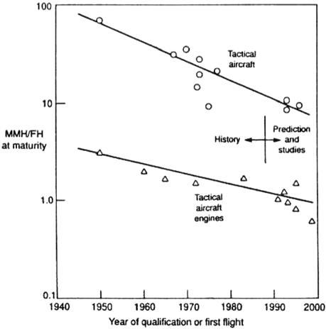
On the surface, the philosophy of testing, analyzing, and fixing appears to be the framework upon which the engine development process is built. Avionics developers have identified the need for more than one pass through the development cycle as a key to reliability improvements. This strategy is referred to as Maturational Development.
In the case of engine development, the Maturational Development approach is totally out of the question, based upon the long lead times involved. A key to supportable engine designs is designing supportability into the components during the earliest phases of component research and development and improving on the supportability throughout the whole technology development process. Care must be taken when integrating these components into a final propulsion system design so that all is not lost in the end product.
A recent supportability success story from GE Aircraft Engines is the T700. In this case, durable/reliable components were integrated into a final engine designed for ease of access and overall maintenance.
The IHPTET initiative demands major performance improvements in our future generations of engines. The challenge facing today’s engine designers is how to reach these performance goals while still improving supportability. The only way to make this happen is for supportability to be a design criterion from the earliest component research and development projects through preliminary design, demonstration, and production. This case outlines an approach to the design of an easily supportable engine.
Advanced Materials
Advanced materials are the most important element in the IHPTET initiative. The supportability community, like the design community, must recognize this fact. Metal matrix composites, ceramic matrix composites, intermetallic compounds, high temperature titanium alloys, sapphire fiber reinforced nickel aluminides, and carbon-carbon will be a way of life. Material costs will dictate net shape manufacturing techniques that are still to be defined. Repairability of these materials is still a question at present. Most of the advanced metallic materials will be powders in their initial manufacturing states. It is envisioned that intricate parts, which are currently castings fabricated from molten metals, will initially be injection molded powder slurries—dried, hardened, and sintered into metallic form. Welding will be replaced by applying a putty-like intermetallic compound and then sintering locally to cure the “weld.” Fiber reinforced matrices will be manufactured by either a metallic spray over ceramic fibers or by layers of metallic foil interspersed with layers of ceramic fibers. In either approach, the final step will be fusion by the Hot Isostatic Press (H.I.P.) process.
Proper attachment methods (bolts, flanges, etc.) are currently being defined or developed. Material strength, ductility, and rupture properties may be different in all three directions. It may be possible to repair “weld” a component in the longitudinal direction but not in the transverse direction. The title “metallurgist” may become obsolete; “materials engineer” will probably be a more apt description.
Engine Preliminary Design
General Approach
Attaining the high thrust-to-weight goal will be accomplished by integrating all engineering disciplines. It is estimated that 50% of the goal will come from new materials, 35% from design innovations, and 15% from engine performance (aerodynamic and thermodynamic) advances. Improved engine performance will be helped by higher efficiencies and turbine inlet temperatures. Design innovations will include multifunctional components, high temperature lubricated bearings, 360° static structures, and design simplicity. Fiber-reinforced metal matrix composites (silicon carbide and sapphire fiber), carbon-carbon (C-C), ceramic matrix composite (CMC), intermetallics, and high temperature titanium alloys will be the new materials for future, very advanced, lightweight fighter engines.
The conceptual engine design process begins with the clear enunciation of the requirements. Before the first cycle calculation has been made, the Design Management and Design Team must understand the requirements for performance, weight, cost, and supportability. Requirements for reliability, maintainability, and repairability must be emphasized and given “teeth” by the Design Management.
Engine considerations are initiated with the engine stick flowpath. The “stick” flowpath is a sketch the preliminary engine designer receives from the aerodynamic designers. The engine preliminary designer must know all engine design disciplines and be able to modify the engine flowpath without violating the design intent or engineering laws. The engine preliminary designer at this point must (1) produce a concise compact fan, compressor, combustor, turbine, augmentor, and exhaust nozzle flowpath, (2) mentally and physically determine component mechanical configuration, and (3) determine module configuration. At this point, the preliminary designer must be permitted to struggle alone as he addresses the engine design goals of performance, cost, weight, and supportability.
Once the designer sets design direction involving all design disciplines, the engine’s initial design configuration begins. The skill with which the preliminary designer understands and balances the often-conflicting requirements as he sets the design direction can have a major influence on the supportability characteristics of the final design. If supportability isn’t considered here, it can conceivably be locked out of the final product.
Specific Approach
The crucial first step in the preliminary mechanical design of an engine is the configuration of the sumps and bearings supporting the rotors. Grossly miscalculate initial rotor dynamics and the preliminary design is time wasted. Current engines have multipiece sump, seal, and bearing configurations requiring manual build-up at engine assembly. Future engines will be lubricated by high temperature lubricants with design simplicity as a top priority. Sumps will be one-piece cartridge bearings and seal configurations for easy assembly, maintainability, and removal. The quick replaceability of the cartridge bearing is an example of design simplicity and supportability interaction.
Once the sumps and shafts are in place, remaining engine components can be wrapped around them, starting with the combustor and rotors. Fan, compressor, and turbine rotors are located relative to the bearings as dictated by preliminary rotor dynamic analysis. Advanced compression rotor systems are simple, integrated, lightweight disks and blades called blisks. Compressor blade replaceability is a maintainability tool eliminated by blisks; but to compensate, the rotors will be tolerant of substantial imbalance and will have rugged, damage tolerant, low aspect ratio, high-pressure rise airfoils, and a minimum number of compression stages. Finally, the casings, shells, augmentor, and exhaust nozzle are added to form an initial engine configuration.
Initial Layouts
Once the responsible designer has received and understands the requirements, has initial cycle data in hand, and has held an initial consultation with all design disciplines and management, a series of configuration options should be created by the designer, the designer-draftsperson, and a small team. Modularity and simplicity should be the guidelines. Upon completion, each configuration is critiqued by the full design group and management. These initial layouts will merely be first attempts to incorporate past experience and design practices, but they should also be allowed to contain the new and creative ideas that have been waiting for a home. During this phase of the design process, the drafting room population should be kept to a minimum except when critiques are invited. Supportability interests and considerations, such as modularity, multifunctional components, ruggedness, accessibility, etc., must be given the same emphasis as the other “traditional” requirements during this critique and iteration phase.
Specific Examples
Overall Engine
Supportability must be designed into the engine in the preliminary design phase, preferably with little or no increase in engine weight or cost. There must be a game plan for assembly, disassembly, and module selection. Figure 19–33 illustrates a schematic of an engine on an assembly dolly. Here major module assemblies such as the augmentor and exhaust nozzles, fan duct, low pressure turbine, and fan and fan frame are mounted and attached to mini dollies so that after disconnecting electrical and service lines, engine axial disassembly can be attained as illustrated in Figure 19–34. Rapid access to the high-pressure turbine and combustor module is attained.
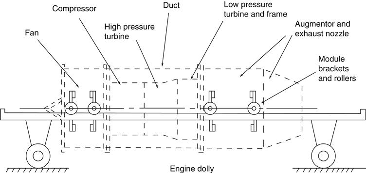
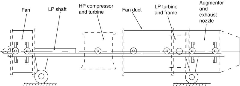
This type of disassembly/assembly is considered highly desirable in many military scenarios.
The engine core or high pressure section of a turbofan engine, normally a small volume portion of the engine, can be rotated vertically in the dolly for further access to either the high pressure turbine or compressor modules and the compressor rear frame assembly. This engine disassembly approach is nothing new—it has been with us for years. This principle was in General Electric’s J-85 engine design, which now has seen 30 years of service.
Component Design
Figures 19–35 and 19–36 show specific examples of how the maintainability aspect of supportability can be incorporated in the engine in the preliminary design phase. The advent of new composite materials allows the designer to custom tailor materials for specific maintainability problems. Figure 19–35 illustrates a conventional shaft spline detail complete with interference fit pilots. Conventional design practice requires pilot interference fits of 0.0005 inches per inch of pilot radius and special tooling to assemble/disassemble splined components (see Figure 19–37).
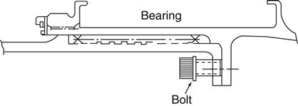
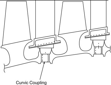
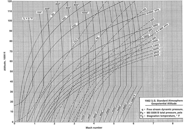
This brute force assembly technique has been effective for past rotor designs using monolithic, metal rotor materials, but requires simultaneous heating and chilling or large special tools. However, this technique is antiquated when applied to advanced design rotors of different materials operating at elevated temperatures. By selecting the material of the respective shafts, the thermal growth coefficients can be matched so a loose fit or snug close tolerance pilot fit is obtained at assembly room temperature and a very tight interference fit, caused by differential radial thermal growths, is achieved at pilot/spline operating temperature. This simple, old, but effective technique, where applicable, can be applied throughout the engine, thus eliminating the use of large and heavy special tooling and allowing the use of simple techniques such as “backoff” bolts, as illustrated in Figure 19–35. These simple tools can either remain on the engine or fit in a mechanic’s standard toolbox.
Controlled shaft heating is another feature available when splined shafts have mismatched thermal growths. Selective heating of the inner shaft by a portable electric heater causes inner and outer shaft relative axial growth, unseating the locking nut for easy nut removal. This simple concept, if properly controlled, eliminates the need of heavy load cells or torque multiplier wrenches for rotor assembly/disassembly.
A second simple, but effective, design assembly/disassembly feature is the old technique of “lead-ons” to protect critical and fragile engine sump seals and other components. For decades engine sumps have been designed as an assortment of small components, hand assembled at engine assembly and requiring interim special dimensional checks. More recent engine sump designs have eliminated special assembly dimensional checks but still require delicate assembly procedures. Why not design the bearings, seals, oil jets, and other related components as a one piece mini module? This principle has been accomplished in electronic design—it’s called the circuit board, used extensively in television sets.
If special lead on procedures for components are required, “lead on” rods are a simple and effective method that (1) if left on the engine add little weight, and (2) if removed can fit in a mechanic’s tool box. Long rods or pins, attached via flanges to the engine casing, allow a “lead on” to protect the sumps, shrouds, or other critical components at assembly/disassembly. A circumferential series of rods or pins, with long protrusions, are rigidly attached to one component and engage with and align a second component prior to engagement of the respective component sump seals, rotor shrouds, or other critical parts. A design such as this requires reasonable, but not special, care at assembly.
Another design detail that can be utilized in the preliminary design phase is the old design friend, the curvic coupling. The use of engine compressor blisks (integral one piece disks and blades) reduces compressor rotor weight but can add difficulties to rotor blade repairability; and, in some instances, impairs compressor rotor accessibility by eliminating the compressor split casing. This one piece casing unit can further reduce engine weight. Therefore, another method must be devised for compressor rotor accessibility, and curvic couplings are an example of this.
As stated in Specific Examples—Overall Engine, the engine core module of a turbofan is a small volume and could be rotated vertically in the engine dolly. By machining curvic couplings into the compressor blisk ends, the compressor rotor can be held together as one piece by a single tie bolt. The T700 compressor rotor is a blisk design held together in this manner. Figure 12–36 illustrates the rotor blisk curvic coupling feature. With the engine core module in the vertical position, heat can be applied to the core rotor tie bolt shaft, inducing shaft axial growth and unloading the nut. With the axial load reduced or eliminated, the coupling nut can be removed.
A final example to aid engine supportability in the preliminary design phase is the design of engine static components. Static components in advanced engines account for approximately 60% of the weight. Engine supportability can best be served by minimizing potential problems. There can be no frame problems if there are no frames. Designing 360°, one-piece, multi-functional components that perform functions previously required by two or three units not only saves engine weight but also minimizes supportability problems by component elimination.
In summary, the US military services are participating with the aircraft engine industry in an ambitious program to develop high performance engine technologies for advanced future military applications. This radical program, starting from a “clean sheet of paper,” is a golden opportunity to integrate many radically advanced but fundamentally correct engineering disciplines, including supportability, into future, very high thrust-to-weight fighter engines. The thrust-to-weight ratio goal is double that of current military engines under development and almost triple the thrust-to-weight ratio of fighter engines currently flying. This accomplishment, scheduled for completion in 15 years, will require the total cooperation and understanding between management, supportability, and engineering. Engine supportability techniques may change but fundamental basics will apply. New materials, not yet commercially available, must be understood. The preliminary design engineer will always be a radically thinking, analytically oriented person with his/her head in the clouds; and the supportability engineer will have both feet on the ground beset with day-to-day problems. Some technical crossbreeding between both will be necessary to meet the supportability challenges of the future.