11.9 Potentiometers and bridges
D.c. potentiometers may be used to measure a direct voltage by comparison with the known ratio of the e.m.f. of a Weston standard cell or electronic solid state reference device. The methods of achieving the linear ratio between the unknown p.d. and the standard-cell e.m.f. are by successive approximation to the balance condition (a) using groups of matched resistors, (b) using opposed m.m.f.s between matched windings and current-ratio resistors (comparator potentiometer), and (c) pulse-width modulation (ratio of time interval). The d.c. potentiometer is a ratio device of high precision with the uncertainty of the standard voltage source limiting the ultimate accuracy.
11.9.1.1 Weston standard cell
The highest quality saturated mercury/cadmium-mercury cell has an e.m.f. of about 1.018 620 V at 20°C. The net e.m.f./temperature coefficient is about −40 μV/°C, arising from the two different coefficients of the limbs, each of the order of 350 μV/°C. It is, therefore, important to avoid a temperature differential across the cell by mounting it in oil or air within a constant temperature enclosure (e.g. for 20°C ± 10 m°C, the uncertainty can be only ± 0.4 μV).
Standard cells are stable, the e.m.f. falling by, perhaps, 1 μV per year. For accurate work, regular confirmation of the e.m.f. should be made at an accredited calibration laboratory.
The internal resistance is 600–800Ω. The current drawn from a cell should ideally be zero: in practice it should be limited to a few nanoamperes for a few seconds.
Should a cell be compared with an electronic solid state voltage reference (below), the cell must be presented and removed while the electronic source is switched on.
11.9.1.2 Electronic solid state e.m.f. reference
These devices use the constant voltage property of Zener diodes to deliver highly stable d.c. voltages, usually at 1 V and 10 V levels for direct voltage meter calibrations, and 1.018 61 V to simulate a Weston cell for d.c. potentiometric standardisation. Up to four diodes (each stabilising at about 6.3 V) are used, having been carefully selected for stability, low noise and low temperature/voltage coefficient properties. After further ageing, these temperature-stabilised monolithic devices may be used either separately with a carefully designed operational amplifier, or connected in cascade in specialised networks to achieve the required output p.d. by potential division using highly stable resistors.
It would appear that these devices are excellent transportable standards of voltage (which should be reliable to within 2 μV/year) and they are much more convenient than Weston cells in this respect. Except for the most extreme requirements of accuracy, they could be used as laboratory standards, provided that at least three separate units are available for intercomparison. With more experience and/or minor refinement to these devices, they could shortly replace the Weston cell completely, since at present the Weston cell can be used as a transportable standard to less than 0.5 μV, but only if very great care is exercised.
Typical electronic devices can deliver, say, 5 mA, 10 V from 2 m Ω and 1.0186V from 2k Ω.
11.9.1.3 Potentiometer principle (using groups of matched resistors)
In Figure 11.21 AB is a manganin wire of length a little greater than 1 m, through which the current I from a 2V secondary cell may be varied by means of R. The current is adjusted so that the p.d. between points F and D, 1.0186 m apart, balances the e.m.f. of the Weston standard cell, the balance condition being obtained by use of the switch S and galvanometer G. The volt drop along the wire is now 1 mV per mm length. The switch S may now be set to apply the unknown voltage Vx, and a new balance point H found. Then the length DH in mm represents the unknown voltage in millivolts.
This very simple arrangement is inconvenient in practice. It suffers also from the disadvantage that the precision of the voltage measurement depends upon the precision with which the point of contact of the slider is known. For example, if the length DH is known only to the nearest millimetre, the precision of the voltage measurement would, in general, be less than 1 in 1000. Much greater precision than this is often required, and to obtain it (and to secure a more compact form of apparatus) some elaboration and refinement in the circuit elements is required. Many practical forms of d.c. potentiometer have been devised.
11.9.1.4 Practical potentiometer
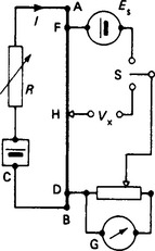
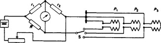
The potentiometer in Figure 11.22 is supplied across AB from a 2 V secondary cell through a rheostat R. Resistors R2, R3 and R4 are connected in series between A and B, but the conditions first considered are with R4 short circuited by the switch at P1. The resistor R3 is divided into equal sections with 19 tappings brought out to studs, and there is an additional stud connected to a tapping on R2.
One terminal of the standard cell is connected to a tapping on the parallel resistor R1, and the other terminal may be connected (when the switch S is in the left-hand position and the key K is depressed) to the point B through galvanometer G. A balance may be obtained with the standard cell by adjusting the rheostat R, and the resistance values are such that the p.d. between successive studs on R3 is then precisely 0.1 V, and the voltage between A and B a little over 1.8 V. In parallel with the shunting resistor R2 is the slide wire W. The tapping on R2 enables a true zero, and small negative readings, to be obtained on W. By suitable choice of the resistance of R2 and W the voltage range covered by the whole slide wire is a little over 0.01 V.
R6 is a tapped resistor with 10 equal sections and 11 studs. The total resistance of R6 is made equal to the resistance of two sections of R3, and R6 always spans two sections by means of sliding contacts on the R3 switch as shown. The total resistance of R6 and two sections of R3 in combination is therefore always equal to a single section of R3 and the potential difference between successive tappings on R6 is then 0.01 V.
The unknown voltage Vx is applied to terminals connected through the galvanometer switch S to the sliding contact on W and to the tapping on the R6 switch. If the slide-wire dial has 100 divisions, each division represents 0.0001 V. Thus, for the switches in the positions shown, Vx might be 0.2376 V. The maximum Vx readable, assuming that there are some graduations provided beyond the 0.01 position on the slider dial, is 1.7 + 0.1 +0.0100 = 1.8100 V.
The resistors R4 and R5 are introduced into the circuit by opening switch P1 and closing P2; this reduces the p.d.s in the potentiometer circuits to one-tenth of those marked. One division on the slider dial would then correspond with 0.000 01V or 10 μV.
Medium- to high-precision potentiometers include a ‘standard cell setter’ so that the actual e.m.f. of the standard cell can be used for standardisation and, subsequently, for rechecking the standardisation during use without altering the measuring dials: this is more convenient, although less accurate than standardising against the dials. The contact T could be the slider of a 10-turn voltage divider with an indicated range, e.g. of 1.018250 to 1.018 750 V in 1-μV steps.
D.c. potentiometers of very high precision have a ratio non-linearity of ±5 parts in 106. A stable current of 50 mA must be provided by an electronic controller, and a high-gain low-noise detector is necessary: this may be a photocell galvanometer amplifier with a display sensitivity of 5000 mm/μV in a 10-Ω circuit.
11.9.1.5 Comparator potentiometer (using m.m.f. balance)
The comparator potentiometer is one of a group of precision bridges employing mutual-coupled inductive ratio arms. The bridges exploit the high m.m.f. linearity and discrimination of a constant current in a variable number of turns.
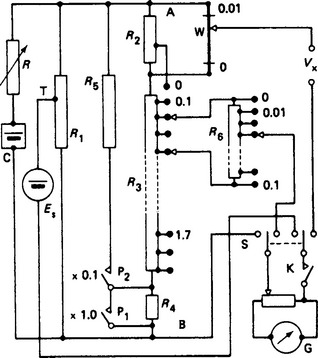
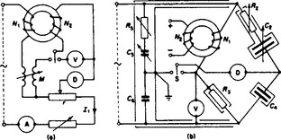
A simplified network is shown in Figure 11.23. The measuring loop M is magnetically coupled to the balancing loop B by the turns Nm and Nb, respectively, on a magnetic core, which also carries a feedback winding with Nf turns. The feedback network includes an a.c. modulated sensor which actuates an a.c./d.c. electronic control network Cb to change the direct current Ib until a zero m.m.f. condition is achieved in the core.
11.9.1.6 Operation and standardisation
If Im and Nb are constant, then for an automatically maintained m.m.f. balance NmIm = NbIb it follows that linear changes in Nm result in corresponding linear changes in Ib. As Nm has in effect a discrimination and linearity of about 1 in 107, these properties are imposed also on Ib. To convert this linear current scale to voltage across Rb, the instrument has to be standardised against a standard cell. The cell, of e.m.f. Er, is connected (through S1) in opposition to the p.d. across Rm, and balance achieved by use of the adjustable direct-current controller Cm, which is then left to maintain this current level.
The equivalent cell e.m.f. ImRm is now connected (through S2) in opposition to IbRb, and Nm turns are selected to be numerically equal to Er. The m.m.f is balanced automatically by the feedback control system and by a small adjustment to Nb so that ImRm = IbRb = Er, represented numerically by Nm. With switch S set to S0 the unknown p.d. Vx is presented through Sx and galvanometer G1 in opposition to IbRb and balance achieved by manual adjustment of Nm. Then Nm is numerically the unknown voltage.
Instruments of this kind are probably the most linear d.c. potentiometers available. They incorporate additional windings that enable the linearity to be checked by the operator. While the actual values of Rm and Rb are not of first importance, it is vital that they should be constant. Resistors are incorporated for subdivision of Im for lower decades of Nm in order to simulate the 107 turns implied by a discrimination of 1 in 107, but they do not contribute unduly to the overall non-linearity, which is about ± 0.3 × 10⁻⁶ of full scale. The system uncertainty must include that of the standard cell, at least ± 1–2 μV.
11.9.1.7 Pulse width modulation potentiometer12
This method subdivides a known stable d.c. voltage in terms of a time-period ratio. If a standard voltage source Er is repeatedly connected to a low-pass filter through a very-high-speed semiconductor switch for a time t1, and then disconnected for an additional time t2, the high-frequency rectangular, chopped waveforms will, after smoothing, give an output E0 = Er·t1/(t1 + t2) with t1 + t2 = T, a constant period. The time ratio can be precisely set using a variable time-interval counter for t1 and a fixed-period counter for T, with each counter being driven from a common highly stable crystal-controlled oscillator. An unknown voltage Vx, in opposition to E0 through a galvanometer, can be measured by variation of E0 (through the voltage-scaled setting of the t1 counter) until galvanometer zero balance is achieved. The e.m.f. Er of the solid state source of steady voltage must be known accurately and the source must be capable of delivering small current surges into the low-pass filter without any significant change in voltage. Conversely, Vx and Er could be interchanged when Vx > Er.
One d.c. variable-voltage source uses the accurately determined voltage as input to constant gain d.c. amplifiers (designed for decade steps) to give a wide-range d.c. voltage standard source with ±50 p.p.m. uncertainty (3-month stability) up to 1.2 kV with a 25 → 10 mA (at 1 kV) current capability and 0.5 → 3.0 s settling times.
11.9.1.8 Applications
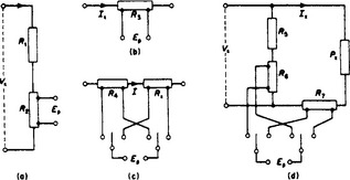
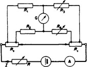
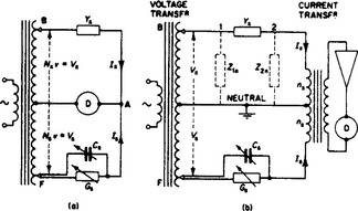
The d.c. potentiometer may be used to determine temperature by measuring the thermo-e.m.f.s in calibrated thermocouples. In conjunction with standard four-terminal resistors and shunts it is applied to the calibration of voltmeters, ammeters and wattmeters, and for the comparison of resistors. In Figure 11.24 the values Vx, Ix, Rx and Px are unknowns, and Ep is measured by the potentiometer. Resistors R1 …, R7 have known values. At (a) a voltage divider is used to measure Vx, and at (b) a shunt is employed to measure Ix. At (c) Rx is compared with R4 by means of their respective p.d.s. The network (d) enables the power Px = VxIx to be determined from Vx and Ix. The resistance of four-terminal resistors is known between the potential (inner) terminals, and not the current (outer) terminals, which minimises errors due to non-uniform current densities and contact resistances.
The National Physical Laboratory (NPL) designed ‘Wilkins’ resistor is a high-stability, four-terminal, a.c./d.c. resistor available in various decade and other values (Tinsley Co., London) which has an exceptionally low time constant for accurate a.c./d.c. comparator networks, etc.
11.9.2 A.c. potentiometers
The a.c. potentiometer may be used to measure the magnitude of an alternating voltage and its phase relative to a datum waveform. The measurements are normally restricted to sinusoidal waveforms, as the presence of harmonics makes a null balance impossible; and operation is usually confined to a single frequency. One recent instrument (Yorke) is capable of measurements up to audiofrequency, with an uncertainty approaching ± 0.05%. The general principles of the Larsen and Gall potentiometers are set out below.
11.9.2.1 Larsen potentiometer
The primary winding of a variable mutual inductor is connected in series with a tapped resistor to a source of voltage V. The unknown voltage Vx is normally derived from the same source, because identity of frequency is essential. The supply current I is controlled by resistor R1 and indicated on an ammeter. The inductor secondary e.m.f. in series with a tapped fraction of the volt drop across R is balanced against the unknown Vx (Figure 11.25) by means of the vibration galvanometer G, the sensitivity of which can be varied by resistor R2. If M and R are the mutual inductance and resistance values at balance, then
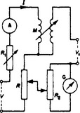
where φ is the phase angle between Vx and I. In practice it may be necessary to reverse either or both of the component voltages to secure balance, and reversing switches are incorporated for this purpose. The mutual inductor should be astatic, to avoid pick-up errors.
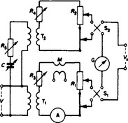
11.9.2.2 Gall potentiometer
The Gall potentiometer (Figure 11.26) provides two quadrature voltage components, summed and balanced against the unknown Vx. The supply voltage V is applied to the primaries of isolating transformers T1 and T2. The secondary of T1 supplies a current, approximately in phase with V, to R1 which consists of a tapped resistor and slide wire in series. The current is adjusted by resistor R3 and read on an ammeter A, and passes through the primary of a fixed mutual inductor M. Any desired value of in-phase voltage (within the available range) is obtained from tappings on R1. The primary of transformer T2 has a series resistor R5 and a variable capacitor C, and may be so adjusted that the current in R2 is in quadrature with that in R1. The exact phase angle, and the calibration of the quadrature circuit, are achieved by balancing the secondary e.m.f. of the mutual inductor M against a fraction of the p.d. across R2. Thus, variable voltages, phase and quadrature, can be obtained from R1 and R2, respectively. These, in series, are balanced against the unknown Vx through the vibration galvanometer G. The reversing switches S1 and S2 facilitate balance and provide for a phase angle over a full 360°.
11.9.3 D.c. bridge networks
A bridge network has as its distinctive feature a ‘bridge’ connection between two nodes, with a null detector to sense the balance condition of zero p.d. between the nodes.
11.9.3.1 Wheatstone bridge
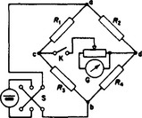
The Wheatstone bridge is an arrangement in very wide use for the determination of one unknown resistance in terms of three known resistances. The network is shown in Figure 11.27, where R1, R2, R3 and R4 are resistors connected at the nodes a and b through a reversing switch S to a d.c. supply. The galvanometer G, with a shunting resistor to control its sensitivity, and the key K are connected to the nodes c and d as shown. R1 and R3 may be set at known fixed values. R2 is a variable resistor and R4 is the unknown resistance to be measured. The bridge is balanced by adjusting the value of R2 until the deflection of the galvanometer, set for maximum sensitivity, is brought to zero. The condition for balance is easily seen to be R4/R3 = R2/R1 and is independent of the voltage applied to the bridge: whence the unknown is R4 = (R3/R1)R2. The bridge may be built up as a single unit with, for example, R1 and R3 each able to be set at one of the resistance values 1, 10, 100 or 1000 Ω. The bridge ratio R3/R1 may therefore have a range of values from 1000/1 to 1/1000. In this case R2 might conveniently be adjustable, by means of dial switches, in steps of 1 Ω from 1 to 11 110 Ω.
The bridge resistors are wound from manganin wire, since manganin is an alloy with a low temperature coefficient of resistance and a low thermoelectric e.m.f. to copper. Any thermoelectric e.m.f.s in the bridge connections which did not on average cancel themselves out could give a false result. Errors from this cause are eliminated by taking a balance for each position of the changeover switch S and using the mean of two observed values of R2.
High-precision Wheatstone bridges are capable of measuring resistances between 1 Ω and 100 MΩ with uncertainties which vary between 5 and 100 in 106 of the reading over this range of values. Modern resistors are very stable devices and they should not change in value by more than a few parts in 106 per year; however, it is prudent to check the linearity of resistive bridges regularly, particularly if they are being used to the limit of the original specification. Some bridges have trimming facilities available with the principal resistors, although corrections can always be applied which although tedious, can avoid imposing new resistance drifts on the bridge as a consequence of changing stable resistors.
Various forms of high-quality bridges are used for measuring the changes which occur in resistive transducers. The Smith and Mueller bridges, used for measurements with precision platinum resistance thermometers, can yield 0.001°C discrimination in readings. For strain gauge transducers there are portable bridges that can detect changes of 0.05% or less.
11.9.3.2 Kelvin double bridge
The Kelvin double bridge is an adaptation of the Wheatstone bridge which may be used for the accurate measurement of very low resistances, such as four-terminal shunts or short lengths of cable. In the network (Figure 11.28) Rx is the unknown and Rs is a standard of approximately the same ohmic value. The two are connected in series in a heavy-current circuit (e.g. 50 A for Rs= 10m Ω, giving 0.5 V drop and adequate sensitivity). Suitable values for R1, R2, R3 and R4 are in each case a few hundred ohms. To use the bridge, R1 and R2 are made equal; then R3 and R4 are adjusted (keeping R3 = R4) until balance is achieved. Then the balance condition is Rx/Rs = R4/R2 = R3/R1. Provided that it is short and of adequate cross-section, the connection between Rx and Rs does not affect the measurement.
Good-quality commercial bridges claim an uncertainty of about ±0.05% for unknowns between 1 Ω and a few micro-ohms. Near the latter level a small constant resistance becomes a limitation. As R1, …, R4 constitute a Wheatstone bridge network, a Kelvin bridge is often extended to measure two-terminal resistances up to 1 MΩ with an uncertainty of ± 0.02%.
11.9.3.3 Digital d.c. low resistance instruments
Digital milliohmmeter/micro-ohmmeter instruments have built-in d.c. supplies; they are auto-ranging and make four-terminal measurements by internal comparator-ratio techniques to give, e.g. 4![]() -digit displays in the case of the Tinsley 5878 micro-ohmmeter with 0.1 μΩ best resolution and uncertainty ± (0.1% → 0.3%) of reading. Also, a IEEE 488 bus attachment is available for use in automated test systems. Thermal e.m.f. balance is incorporated as well as lead compensation.
-digit displays in the case of the Tinsley 5878 micro-ohmmeter with 0.1 μΩ best resolution and uncertainty ± (0.1% → 0.3%) of reading. Also, a IEEE 488 bus attachment is available for use in automated test systems. Thermal e.m.f. balance is incorporated as well as lead compensation.
11.9.3.4 Comparator resistance bridge
The comparator resistance bridge is a variant of the comparator potentiometer (Figure 11.23). In this case the network connections and adjustments are such that, at balance,
where Rb is the known standard four-terminal resistor and Nb has been adjusted to make Rb/Nb an exact decade value. The unknown four-terminal resistance Rm is found in terms of a number of turns Nm and a decade factor.
The two resistors can be compared at different current levels, so that, for example, the rated current can be used with the test resistor, while the standard resistor can be used at a current well below the level at which self-heating effects would change its resistance value. The actual comparison uncertainty with this class of bridge is less than 1 in 106, to which must be added the basic uncertainty in Rb, probably 2 in 106 if it is a class ‘S’ (or ‘Wilkins’) standard four-terminal resistor known to be stable.
11.9.4 A.c. bridge networks
A.c. network parameters (impedance, admittance, phase angle, loss angle, etc.) can be measured in the following ways:
(1) Single-purpose or multipurpose a.c. bridge networks, with four or six arms or with inductive ratio arms.
(2) Analogue and digital networks developed for special applications and consisting of frequency-selective or resonant or filter networks; they are associated usually with measurements at radiofrequencies and high audio-frequencies.
(3) Digital multimeter instruments for measuring the modulus of the unknown parameter (but not other qualities).
The treatment in this subsection is confined largely to (1).
11.9.4.1 Balance conditions
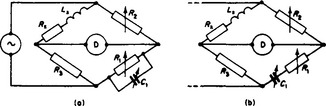
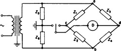
In the four-arm bridge of Figure 11.29, the arms comprise impedance operators Z1, Z2, Zs and Zx. The network is supplied at nodes a and b from a signal generator, and a sensitive null detector is connected between nodes c and d. If Z1 and Z2 (fixed standards) and Zs (variable standard) are so adjusted that the p.d. between c and d is zero, then the unknown impedance Zx depends on whether Z1 and Z2 are adjacent as in Figure 11.29(a), or in opposite arms as in Figure 11.29(b); in either case the balance condition is that the product of pairs of opposite arms is equal, giving
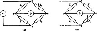
where Ys = 1/Zs. These are complex expressions, so that the equality involves both magnitude and phase angle; alternatively, both phase (‘real’) and quadrature (‘imaginary’) components. Thus, equation (a) above can be written in terms of magnitudes in either of the following ways:
The bridge arms will include intentional or stray inductance and capacitance, and the corresponding reactances are functions of frequency. Most practical bridges are so chosen that only two or three final adjustments are necessary to obtain the optimum null condition of the detector.
11.9.4.2 Signal source
The bridge supply can be from a screened power-frequency instrument transformer, but more probably from a fixed- or variable-frequency signal generator (see Section 11.7.4). A voltage up to 30 V may be required, but a few volts is normally adequate, especially for radiofrequency bridges. The maximum power of a signal generator is of the order of 1000 mW, so that to avoid overload and distortion it is important that the appropriate voltage be set and a reasonable match be obtained between the generator and the effective input impedance of the bridge network.
11.9.4.3 Detector
A moving-coil vibration galvanometer may be used at discrete frequencies over the range of 10 Hz–1.2 kHz. The galvanometer has a taut suspension mechanically tuned to the operating frequency. The method is sensitive, and effectively filters harmonics, but it is often more convenient to employ the electronic detectors included in most commercial bridges. These include tuned-resonance amplifier networks or broad band high-gain electronic amplifiers; both give a rectified out-of-balance display on a d.c. instrument, with ‘magic eye’ or c.r.o. as possible alternatives. In some portable instruments it was the practice to use head-telephone sets, which are highly sensitive in the audio range of 0.8–1.0 kHz.
11.9.4.4 Bridge-arm components
Precision a.c. resistance boxes can be designed with very low time constants. They are available with switched or plugged groups of ten resistors in decade values between 0.1Ω and 1 MΩ. Careful construction and screening enable some of these devices to be used at frequencies up to 1.2 MHz before the residual reactance becomes significant. An overall uncertainty of ±0.05% is possible, but 0.1–1.0% is more conventional. (See also Section 11.9.1.8.)
Multi-dial switched mica capacitors are available with good stability and low loss tangent. Single- and double-screen capacitors have respectively, three and four terminals, and care is needed to avoid unwanted stray capacitance, the screens being maintained at the proper potentials with respect to the equipment and the environment.
Continuously variable calibrated air-dielectric capacitors with ranges between 20 and 1200 pF are used for small adjustment, and ranges of fixed or variable mutual inductors are available. For high-voltage bridges the standard capacitors are of fixed value, and designed with air or compressed gas as dielectric for 300 kV and above.
11.9.4.5 Low-frequency and audiofrequency bridges
A selection is given of the more important bridges, many of which form the basis of commercial instruments; for example, the inductance bridges of Maxwell and Hay, the modified de Sauty bridges for capacitance, the Schering bridge for capacitance and toss tangent at low and high voltages, and the Wien bridge for frequency and a.c. resistance. These bridges are commonly made to give results with a ±1% uncertainty, but can be designed for ±0.1%.
All bridges should be checked occasionally to show that the reference standard components have not changed and that the range and ratio division has not drifted; also, if the bridge is frequency sensitive, the frequency of the oscillator and the drift rate should be investigated. Naturally, superior standard components must be available which have recent ‘traceability’ certification, in addition to accurately known decade-ratio measurement techniques. Where bridge measurements are implicit in contract specifications, it may be prudent or necessary to justify the claims by referring the instrument to a calibration service standards laboratory.
11.9.4.6 Mutual inductance
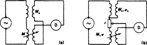
Figure 11.30(a) shows the simple Felici–Campbell bridge for the measurement of an unknown mutual inductance Mx in terms of a variable standard M. For balance on the null detector D, then Mx = M, on the assumption that the inductors are perfect, i.e. that the secondary e.m.f. is in phase quadrature with the primary current. Each, however, has a small in-phase component that can be represented by an equivalent resistance σ. The modification in Figure 11.30(b) shows Hartshorn’s arrangement, which enables the impurities to be measured: at balance by adjustment of M and r, the conditions are Mx = M and σx = r + σ.
11.9.4.7 Inductance
Inductance may be measured by Wien’s modification of the Maxwell bridge (Figure 11.31(a)). If the unknown inductor has an inductance Lx and an equivalent series resistance Rx, balance gives
The advantage is that inductance is measured in terms of a high-quality and almost loss-free capacitor. The bridge can measure a wide range of inductance values with Q factors less than 10. High Q factors require excessively large values of R1, and by creating the same effective phase characteristic by means of a low-valued resistor R1 in series with C1, the Hay bridge of Figure 11.31(b) is obtained. The balance conditions for it are
A disadvantage is the need to measure the frequency.
A commercial instrument using the Maxwell and Hay bridges has built-in supplies at frequencies of 50 Hz, 1 kHz and 10 kHz, and an inductance range from 0.3 μH to 21 kH with an accuracy within ±1%. The loss resistance is known to about ±5%, and it is possible to introduce a d.c. bias.
11.9.4.8 Capacitance at low voltage
Relatively pure capacitors can be measured by the de Sauty bridge (Figure 11.32(a)), the balance condition for which is Cx = Cs(R4/R3). Imperfect capacitors can be compared by the arrangement shown in Figure 11.22(b), in which the imperfection is represented by a series resistance r. To obtain balance, adjustment of all four resistors R is necessary:
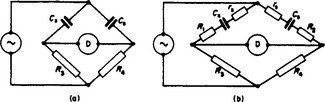
Portable commercial capacitance testers, with battery-driven 1 kHz oscillators and rectified d.c. or headphone detectors, use a modified de Sauty bridge network so that loss tangent can be estimated and the capacitance measured to an uncertainty of about ±0.25%.
11.9.4.9 Capacitance at high voltage
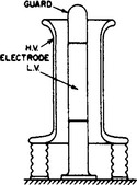
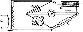
Dielectric tests at high voltages, particularly of the loss tangent, can be made with the Schering bridge (Figure 11.33). The bridge is in wide use for precision measurements on solid and liquid dielectrics, and for insulation testing of cables, high-voltage machine windings and capacitor bushings. The capacitance of the high-voltage standard capacitor Cs is calculable, and with an air or gas dielectric can be assumed to have zero loss. A typical standard capacitor for 150kV is shown in Figure 11.34; for higher voltages the clearances necessary for avoiding corona and breakdown are large, but the dimensions can be reduced by a construction in which the dielectric gas is under pressure.
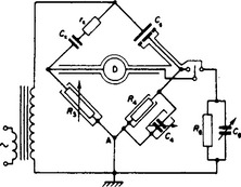
The test capacitor in Figure 11.33 is represented by Cx and a series loss resistance rx. R3 is a variable resistor, and the fourth arm comprises a variable low-voltage capacitor C4 in parallel with a resistor R4 (which may be fixed). Then, for balance
The loss tangent is a valuable and sensitive indication of the quality of the test insulation. If periodical tests reveal a gradual increase in the loss tangent, then deterioration is occurring, the loss power is increasing and breakdown in service is probable.
To avoid electric field coupling between bridge components–-in particular, between the high-voltage electrodes and the connecting leads–-that would affect accuracy, components R3, R4 and C4 are enclosed in metal screens connected to the earthed point A. Again, to avoid errors due to intercapacitive currents between the centre low-voltage electrode and the guard electrode of Cs, these electrodes should be brought to the same potential by aid of the auxiliary branches Cg and Rs. Balance is achieved with the detector switched to this combination, in addition to the main balance. If the test capacitor Cx is a cable with an earthed sheath, or a capacitor bushing on site and not readily insulated from earth, then the bridge node A must be isolated: careful screening is now even more necessary. Figure 11.35 shows the arrangement for a portable Schering bridge equipment for testing an earthed bushing. It will be seen that an earthed screen isolates the bridge from the transformer primary, and a second screen connected to point A keeps capacitive currents from the high-voltage connections out of the bridge arms.
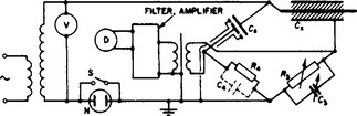
Discharge bridge: This has been developed to detect the onset of void breakdown in cables and bushings. The network (Figure 11.36) can be used to test an unearthed component–-for example, the bushing Cx; the arrangement resembles that of the Schering bridge. The stray capacitances of the guards and screening of Cs act as the capacitance C4, which, however, at the discharge frequencies concerned, is greater than that required for balance. Hence, it is necessary to provide the variable capacitor C3. The bridge output is fed to a rectifier milliammeter D through a filter and amplifier designed to pass, e.g. the band 10–20 kHz, so that the indication is a measure of the discharge current. On the supply side of the bridge is connected some artificial source of discharge voltage, such as the neon tube N, which serves initially to balance the detector D.
11.9.4.10 Wagner earth
Capacitance between bridge arms and earth in the Schering bridge causes disturbing currents to flow so that false balance conditions may result. If, as in Figure 11.37, the bridge supply is not earthed but the nodes c and d are at earth potential, then the detector is also at earth potential and no stray capacitance currents can flow in it. Further, all branch capacitances to earth are stabilised. The Wagner earth method secures this condition by the use of the additional impedances Z5 and Z6, the junction of which is solidly earthed. Z5 and Z6 must be of the same type as either Z1 and Z2, or Z3 and Z4. If balance is achieved for both positions of the switch, then nodes c and d must have the same potential as the earthed junction, which is zero. Stray capacitance at a and b is innocuous as it merely ‘loads’ the supply.
The Wagner earth is usually applied to commercial Schering bridges, but the technique is applicable to any bridge and can be particularly helpful at higher frequencies.
11.9.4.11 Inductive ratio-arm bridge
The principle is explained by reference to the simplified diagram in Figure 11.38(a), the essential features being the coupled windings of, respectively, Nx and Ns turns. If the voltage per turn is v, then the two windings have the voltages Vx = Nxv and Vs = Nsv, respectively. Let Vx = Vs; then the current Ix through the unknown capacitive admittance Yx can be made equal to the current Is by variation of the parallel standards (conductance Gs and capacitance Cs), until the detector shows a null reading. For this condition the standard admittances represent the parallel equivalent network values of Yx. If Yx is inductive, the Cs connection at F is transferred to B to avoid the use of standard inductors, which are very inferior to standard capacitors.
The voltage linearity of the input transformer is of fundamental importance to this class of bridge. With modern techniques and magnetic core materials, it is possible to wind toroidal cores to produce an extremely uniform reactive distribution (leakage inductive reactance and turn-to-turn capacitance) with a resultant non-linearity of about 1 in 107 in the magnitude of the mutually induced e.m.f. per turn.
In one well-known bridge (Wayne Kerr) the primary winding of a current transformer is inserted at A and the detector removed to the secondary winding as in Figure 11.38(b). The two parts of the primary winding (ns and nx turns) are wound in opposite senses and the detector can indicate the zero m.m.f. condition in the windings.
In general, Ns differs from Nx and ns from nx, so that Ixnx = Isns for balance; further, the primary of the current transformer is at the ground (or earth) potential of the neutral if the trivial resistance drop of the windings is ignored, so that Ix = (Nxv) Yx and Is = (Nsv) Ys. Combining these results gives
The double turns ratio product can be used to permit one accurate standard resistor or capacitor to be switched to any Ns turns of value 1–10 to simulate ten accurate standard components by the precise selection of turns. Moreover, wide-range multiplication of the simulated standard is achieved by decade tappings on Nx and nx.
An important advantage with this class of bridge is the possibility of connecting the neutral to earth; then small leakage currents from Yx to earth are almost completely eliminated, since the current transformer is at earth potential and any small leakage currents from the high-voltage side of Yx merely cause a slight uniform reduction in v but does not alter the turns ratio. Hence, determinations such as the following are possible:
(1) One-port low-capacitance measurement in the presence of a large shunt capacitance due to connecting leads.
(2) One-port in situ impedance measurement, the effect of the remainder of the network (shown dotted in Figure 11.38) is neutralised.
(3) Three-terminal impedance transfer functions for correctly terminated networks.
The results of measurements appear in parallel admittance form, and may require elementary computation to render them into series impedance form, with due regard to frequency. With medium to high values of impedance, resistance and capacitance are unaffected, but for inductance measurement (involving a ‘resonance’ balance) a reciprocal ω2 correction is needed. For low-impedance networks, resistance and inductance are unchanged but capacitance readings require correction.
11.9.4.12 Characteristics
Universal bridges of the inductive ratio-arm type measure over a wide range of values, at an angular frequency of, e.g., 10 krad/s from a built-in oscillator, or at other frequencies up to 10 MHz using external signal generators and tuned electronic detectors. The measurement uncertainty can be within ±0.1–1.0%, provided that the standard component values are trimmed against superior standards and that the actual frequency is measured when frequency sensitive parameters are measured.
The Wayne Kerr precision bridge operates at 1591.55 Hz (ω = 10 krad/s) and the six-figure display has a minimum uncertainty of 0.01%. The instrument uses an electronic null-seeking process to assist the automatic balancing procedure. With external source the bridge has a frequency range of 0.2–20 kHz with manual balancing.
Admittance bridges are commercially available to operate up to 100 MHz. At this frequency lumped parameter measurements are being displaced by distributed-parameter network characteristics.
11.9.4.13 Current comparator bridge
The a.c. current comparator instrument uses current transformers only in the load network. It is based on the principle, of m.m.f. (i.e. ampere-turn) balance on an ideal magnetic circuit, in which the current ratio is the inverse turns ratio.
The two basic current coils, P and S in Figure 11.39, are wound in opposing senses on a common magnetic core with a high initial permeability. The null m.m.f. condition is sensed by winding M and manual selection of the turns ratio Np/Ns. The ideal balance condition can be closely approached in practice by shielding the detector from magnetic leakage by a laminated magnetic screen and by a compensation winding Wc. The shield must not form a short-circuited turn; but it does aid magnetic energy transfer between windings P and S. This is advantageous in current-transformer calibration, as it enables an external burden B to be supported under balance conditions. Any change in the capacitive error due to B can be neutralised by Wc connected on one side of the separate centre-tapped transformer Wb. By careful design the capacitance distribution is uniform.
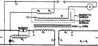
The internal p.d. of the major winding can be neutralised by a parallel compensation winding Wc wound within the magnetic shield, so reducing capacitive currents, as it can be held at earth or reference ground potential.
The commercial range of comparators include d.c. potentiometers, direct voltage and current ratios, d.c. and a.c. four-terminal resistance comparison, voltage- and current-transformer errors, and high-voltage capacitor comparison. All the instruments derived from d.c. and a.c. comparators possess very linear properties, excellent discrimination and good stability. When certified they can be used as comparative reference standards.
11.9.4.14 H. V. capacitance comparator bridge
Standard capacitors used with high-voltage bridges (such as the Schering and comparator types) use compressed gas construction up to a maximum of 1000 pF, although 100 pF is more common. Measurement of such capacitors is based on the principle that a stable alternating voltage to two capacitors produces a current ratio equal to the capacitance ratio. The variable turns ratio of the comparator bridge can be used to balance an unknown capacitor up to 1000 times as large as the standard. By cascading, the range can be extended still further.
11.9.4.15 Substitution
In any active network the equivalent parameters of a component may be measured if variable reference standards can be either substituted for the component or connected in parallel with it–-provided always that the standards can be adjusted so that no final change occurs in the voltage, current, phase or harmonic content of the waveforms in the network. The substitution principle can be applied to any type of bridge, or other class of network; resonant networks often provide the best discrimination between the two conditions. It is important that the stray capacitance, inductance and resistance paths, to earth and between components, should be unchanged by the act of substitution; hence, for the substitution test there should be (ideally) no change in the geometrical layout of leads and components. This can be easily achieved with low-loss changeover switches or coaxial connectors.
For the measurement of radiofrequency components, where shunt capacitance effects are prominent, the substitution principle is particularly valuable. Typical applications are discussed below.
11.9.4.16 Parallel-T network
Figure 11.40(a) shows a general parallel-T network, with an a.c. source as input and a detector across the output terminals. The balance condition (of zero output) in terms of the impedance operators is
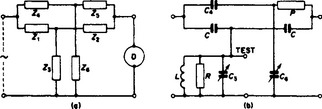
Suppose that Z1 and Z2 are pure reactances of like sign, e.g. –- jX1 and −jX2, and that Z3 is purely resistive, then
which is equivalent to a negative resistance and capable of balancing out a positive resistance in Z4 or Z5. An example is shown in Figure 11.40(b). The source is a modulated signal generator and the detector is, in effect, a radio receiver tuned to the ‘carrier’ frequency. Balance is achieved by variation of C3 and C6 with the test terminals open-circuited. If an unknown admittance Gx + jBx is now connected across the test terminals and the disturbed balance restored by altering C3 and C6 to C′3 and C′6, respectively, then
Bridge screening is simplified because the common source and detector terminal can be earthed. The use of a variable resistor as a balance arm can often be avoided, a considerable simplification for radiofrequency measurement.
11.9.4.17 Bridged-T network
This can be used at frequencies up to about 50 MHz. Figure 11.41(a) shows the schematic arrangement, and Figure 11.41(b) illustrates a common application. If the unknown impedance Zx = R + jωL is such that R2 is negligible compared with ω2L2, then for balance
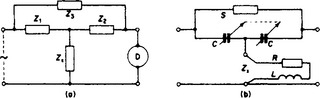
whence R and L can be obtained if the angular frequency ω is known.
11.10 Measuring and protection transformers
Measuring (instrument) transformers are used primarily for changing currents and voltages in power networks to values more suited to the range of conventional indicators. Protection transformers are employed in systems of fault protection. Both types are dealt with in BS 3938 (Current transformers) (IEC 185) and BS 3941 (Voltage transformers) (IEC 186 and 186A).
11.10.1 Current transformers
Air-cooled current transformers (c.t.) are used in circuits of voltage up to 660 V and currents up to 75 kA. The bar primary form employs the actual cable or bus-bar of the main circuit as the primary winding. The core is built of high-grade steel laminations in rectangular or circular shape. The secondary has the appropriate number of complete turns uniformly around the annular core or on all four sides of the rectangular core. The assembly of core and secondary encloses the bar primary, which is equivalent to a single turn.
For lower primary currents it is necessary to provide a conventional primary winding. This gives a better primary/secondary coupling and a greater accuracy.
Current transformers must be insulated to withstand the service voltage, which may be up to 400 kV. Oil immersion may be necessary, in which case the core and coils are clamped to the top cover to facilitate removal as a complete unit.
11.10.1.1 Burden and output
Primary currents have preferred values between 1 A and 75 kA, with rated secondary currents of 5 A and 1 A (also 2 A). The rated burden is the ohmic impedance ZT of the secondary circuit when carrying the rated current Is at a stated power factor. The rated output is the volt-ampere product (IsZT)Is. The rated output, the limiting value for which accuracy statements apply, appears in selected preferred values between 1.5 and 30 VA. The normal operating mode of a c.t. is as a low-impedance device; hence, a short-circuiting switch is provided for the secondary winding for use when a low-impedance load (e.g. an ammeter) is not connected to the secondary terminals.
11.10.1.2 Errors
In an ideal c.t. the primary/secondary current ratio is precisely the same as the secondary/primary turns ratio, and the currents produce equal m.m.f.s in exact antiphase. In a practical c.t. the current ratio diverges from the turns ratio, and the phase angle differs by a small defect from opposition. These ratio and phase angle errors arise from that component of the primary current required to magnetise the core and provide for core loss, and from the e.m.f. necessary to circulate the secondary current through its burden. In transformers intended for accurate measurement and for metering, these errors must be small.
11.10.1.3 Classification
The limits of error define the ‘class’ of transformer. BS 3938 defines six classes for measuring and three for protective c.t.
Measuring c.t: The classes in descending order of accuracy are designated AL, AM, BM, CM, C and D. The limits of ratio error vary from ± 0.1% for AL to ± 5% for D; and the phase error from ±5 min in AL to ± 120 min (2°) in types CM and C, with no limits quoted for type D.
Protective c.t: The classes are termed S, T and X. The limits of ratio error for S and T are, respectively, ± 3 and 5%, and the corresponding phase limits are 3° and 6° approximately. Limits for type X are not stated explicitly. In testing S, T and X classes it is necessary to distinguish between low-and high-impedance types.
11.10.1.4 Measurement
Errors are normally measured by comparison with a c.t. of higher class. By convention, a phase error is positive when the secondary current phasor leads that of the primary current.
11.10.1.5 Arnold method
In Figure 11.42 C is the c.t. under test and B is a standard of the same nominal ratio and having known, very small errors. The working burden of the test c.t. is Z. The network is such that the difference between the secondary currents Ib and Ic flows in the non-reactive resistor R and is measured by means of the mutual inductor M and slide wire r fed by the auxiliary c.t. F (conveniently of ratio 5/5 A). Phase balance is achieved by adjusting M (positive or negative), and ratio balance by selection of r around the centre-tap of P. From the phasor diagram, the components of the difference current I are approximately Ib–Ic and −jIc(βc–βb) because the phase angles are actually very small. At balance the condition is given by Ib(r–jωM) = RI. Equating the ‘real’ parts gives Ic/Ib = 1 – (r/R); whence in terms of the current ratios kc = Ip/Ic and kb = Ip/Ib, where the primary current is common to both c.t.s,
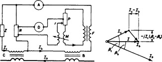
provided that r ![]() R. Equating the ‘imaginary’ parts gives
R. Equating the ‘imaginary’ parts gives
The bridge readings give the errors directly by comparison with those of the reference transformer.
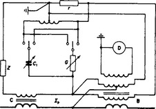
11.10.1.6 Kusters method
This is a comparator method (Figure 11.43) in which C is the c.t. under test with its rated burden Z, and B is an a.c. comparator with the same nominal ratio as C but possessing negligible errors. The errors of C can be deduced directly from the balance settings of the arms of the parallel G – C1 network.
11.10.2 Voltage transformers
Magnetically coupled voltage transformers (v.t.) resemble power transformers in basic principle, and have recommended primary voltages up to ![]() . Oil-immersion is necessary for these levels. The preferred secondary voltages lie between
. Oil-immersion is necessary for these levels. The preferred secondary voltages lie between ![]() and 220 V/ph.
and 220 V/ph.
11.10.2.1 Burden and output
The preferred rated output burdens lie between 10 and 200 VA/ph, and the rated burden is normally the limit for which stated accuracy limits apply.
11.10.2.2 Errors
Five classes are listed in descending order of accuracy, namely AL, A, B, C and D. The voltage ratio error limit varies between 0.25 and 5% and applies for small voltage changes (± 10%) around the rated voltage; and the phase error limits are ± 10 min to ± 60 min from class AL to class C. The phase error of D is not defined.
For dual purpose v.t. (i.e. for both measuring and protective application) additional classes E and F are defined which quote the permitted limits of error for classes A, B and C when used at voltages between 0.05 and 1.9 times rated voltage. The v.t. is then denoted by both relevant class letters. The extended error limits are ± 3–5% and ± 2–5%.
11.10.2.3 Measurement
By convention, a phase error is positive when the secondary voltage phasor Vs leads the primary voltage phasor Vp. The ratio error is (krVs – Vp)/Vp, where kr is the nominal rated transformation ratio. The rated output is stated in volt-amperes at unity power factor for the specified class accuracy.
11.10.2.4 Dannatt method
This deduces the error in terms of network parameters (Figure 11.44). The v.t. primary is fed from a supply to which is also connected the standard air capacitor Cs in series with a low-valued resistor Rs. The v.t. secondary is loaded with the rated burden Z in parallel with a series-parallel network comprising high-valued resistors R1 and R2, a capacitor C1 and the primary of a mutual inductor M. The secondary voltage of the mutual inductor is balanced against the volt drop across Rs. To ensure that the guard and guarded electrodes of Cs are held at the same potential, a variable resistance Rs is connected so that balance is obtained with either position of the switch S. The balance condition is such that the ratio and phase errors are given very closely by
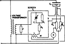
where L is the self-inductance of the mutual inductor primary.
11.10.2.5 Kusters method
The a.c. comparator bridge can be applied. The capacitance ratio of two gas-filled high-voltage capacitors supplied by a common secondary voltage is measured with the currents passing through the separate balancing windings. If one high-voltage capacitor and its series-connected balancing winding are now fed from the primary supply of the v.t., then the voltage ratio can be found by rebalancing the comparator when the two capacitors are connected, respectively, to the primary and secondary voltages.
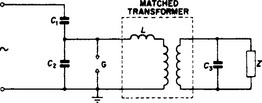
11.10.2.6 Capacitor-divider voltage transformer
For high-voltage transformers for 100 kV and above, a more economical and satisfactory voltage division for measurement and protective purposes is given by use of the capacitor-divider system (Figure 11.45). The reduced intermediate voltage appears across the protecting gap G as the input to a tuned transformer. Changes in the secondary burden Z, which would adversely affect the errors, are minimised by adjusting the transformer leakage reactance and/or that of a series inductor L to resonate with the input capacitance (C1 + C2) effectively across the primary. There is a consequent sensitivity to frequency.
The classification is the same as for magnetic transformers, except that AL does not apply and there is an additional limitation on frequency. The transient performance is naturally significantly different from that of the normal v.t.
11.11 Magnetic measurements
Because of the non-homogeneity of bulk ferromagnetic materials, magnetic metrology is relatively inaccurate and imprecise. The fields of interest lie in the basic physics of magnetism, the distribution of the magnetic field, the assessment of magnetic parameters, and the measurement of core loss.
Physical basis: The origin of magnetic phenomena lies in the statistical quantum-mechanical behaviour of electrons and particles. Additional information can be obtained by photography of domain formation.
Field distribution: Two-dimensional field distributions in air-gaps are readily traced by current-field analogues such as conducting paper or the electrolytic tank. The tank can also be employed for restricted three-dimensional fields, and tests around models or actual equipments can be based on various types of small sensor working into calibrated instruments (fluxmeter or ballistic galvanometer) or a Hall effect device.
11.11.1 Instruments
The most simple fundamental standard of magnetic flux density is based on the accurately known dimensions of a long, uniformly wound solenoid carrying a known current. Alternatively, a uniformly wound toroid can be used, although in this case the flux density will not be quite uniform across the core section. The measurement of flux and flux density can be carried out by means of the ballistic galvanometer or fluxmeter for the former, and the Hall effect instrument for the latter.
11.11.1.1 Ballistic galvanometer
The moving coil of a galvanometer with a long periodic time gives a first swing proportional to the time integral of the current through it (i.e. the charge) provided that the duration is very short. The charge results from a time integral of voltage (i.e. magnetic linkage) impressed on a known resistance. The moving coil is connected in series with a search coil and a resistor, and is immersed in the magnetic field due to a known current. When this current is rapidly reversed, the total change of linkage is presented to the galvanometer as an impulsive charge, and the first deflection of the instrument is used for calibration against a known (or calculable) linkage change, or for measuring an unknown linkage. The main limitations to accuracy are the observation of the scale and the uncertainty in the current measurement. A typical high sensitivity ballistic galvanometer has a period of 20s, a moving-coil resistance of 850 Ω, and a sensitivity of 8.5 m/μC on a scale distant 1 m from the coil using a lamp and mirror technique.
11.11.1.2 Fluxmeter
The fluxmeter is a permanent-magnet instrument with a moving coil of low inertia and negligible control torque. Its damping is made high by use of a relatively thick aluminium former, so that the period is long. It is immaterial whether the time taken to change the linkage in a search coil connected to the moving coil is long or short, and in consequence the instrument is useful in iron testing, where the time taken for a flux to collapse or reverse may be several seconds. The deflection is read from the initial position of a pointer on a quadrant scale when the pointer reaches its maximum deflection; after this the pointer drifts slowly back to a zero position. A typical full-scale deflection would be given by a change of 10 μWb-t.
Strong air-gap flux densities can be measured by an alternative method in which a small coil is rotated at a high and known speed, the induced e.m.f. being proportional to the local flux density.
11.11.1.3 Hall effect instrument
The Hall effect applies to conductors generally, but its application is normally associated with semiconductor materials. These should be of low resistance so that, even for small signals, the thermal (Johnson) noise effects will be low. Bulk materials, indium arsenide and indium antimonide, have low resistances and good output voltage coefficients, with the InSb voltage larger than that of InAs; however, InAs is usually selected, as its temperature coefficient is one-tenth that of InSb. Thin-film InSb is used for switching applications where the higher output e.m.f. is the prime consideration. The Hall effect response is very fast, being usable up to the megaherz range. Bulk material InAs elements are more effective than thin-film elements, owing to the much lower resistances obtainable.
In commercial instruments the current Ic in the sensing element can be a direct current chopped at audio frequency; the resultant audiofrequency Hall voltage EH, after linear amplification and demodulation, can be displayed on a taut-band d.c. moving coil indicator against a calibrated scale of flux density. Typical ranges have full-scale deflections between 0.1 mT and 5T for steady fields. Pulsating fields can be measured with d.c. instruments at frequencies up to 500 Hz with a cathode-ray-oscilloscope detector. Instruments for alternating fields only are available for frequencies of about 30 kHz, with ranges similar to those of d.c. instruments.
An instrument and probe can be checked by use of stable reference magnets, which may have uncertainties of 0.5–1.0%. The overall uncertainty of a scale reading is typically ± 3% of the full-scale deflection for the range.
The sensing elements are protected by epoxy glass-fibre or similar enclosures, and are available in a variety of forms for probing transverse, coaxial or tangential fields. The flat form is most common, typically with the dimensions 0.5 mm × 4mm × 25 mm. Incremental measurements, using two matched probes and backing-off networks, enable perturbations as small as 0.1 μT to be observed either in the presence of, say, a given 0.1 T field or as a difference between two separate 0.1 T field systems. Hall effect instruments have many obvious applications where the magnitude and direction of the field distribution is required such as air gaps of machines and instruments, magnetron magnets, mass spectrometer fields, residual interference fields, etc.: in addition, the Hall-effect principle can be used in a variety of transducer applications by making Ic and B proportional to separate physical functions, and measuring the instantaneous or average results of this product. One example is a wide band, 50 kHz wattmeter in which Ic and B are made, respectively, proportional to the scalar values of the load current and voltage.
11.11.2 Magnetic parameters
The d.c. magnetisation curve, hysteresis loop and relative permeability can be obtained by use of a fluxmeter or calibrated ballistic galvanometer, using a method substantially the same as for calibration. The magnetic test material constitutes the core of the toroid, or is built in strips to form a hollow square. The a.c. cyclic magnetisation loop differs from the ‘static’ loop, and is still further modified when a d.c. bias m.m.f. is superposed. The a.c. loop can be viewed on a c.r.o. displaying the B and H functions on the Y and X axes, respectively. The H function can be obtained from the volt drop across a small resistor carrying the magnetising current, and the B function from the time integral of the search-coil voltage obtained with the aid of an operational amplifier.
11.11.2.1 Core loss
In a low-frequency test the loop area of the B/H relation is directly proportional to the core loss per cycle of magnetisation, which provides a simple comparative test for specimen material. A more convenient method employs low power factor wattmeters, but care is needed to exclude instrument and connection losses. Selected samples of sheet steel intended for the cores of inductors and power transformers are prepared for testing in the form of strips (e.g. 30 cm × 3 cm) assembled in bundles and butted or interleaved at the corners to form a hollow square. The sides are embraced by magnetising and search coils of known dimensions. Input power and current, and mean and r.m.s. voltages, are read at various frequencies and voltages to assess the overall power loss within the material and (if required) an approximate indication of the eddy and hysteresis loss components. The Lloyd–Fisher and Epstein squares are commonly used forms, the latter being referred to in BS 601 (Sheet steel).
The magnetic properties of bars, forgings and castings are derived from galvanometer or fluxmeter measurements (BS 2454). A.c. potentiometer and bridge methods are also used, especially for low-loss materials at frequencies in the audio range. With ferrite and powder cores, as with Q-value tests of a coil with and without a slug core, r.f. resonance methods are convenient.
Production and quality control test equipment for core-loss and coil-turns instruments include a ‘coil-turns tester’ (Tinsley 5812D) with a four-digit display of the number of turns in non-uniform and uniform windings, by using an inductive comparative measurement against a standard winding: the same range of ‘magnetic type’ instrumentation includes a ‘shorted-turns tester’ which will detect single and multiple shorted circuited turns in coils of any shape or number of windings; while a ‘core tester’ can check transformer core characteristics of EI stacks, C cores and toroids including hysteresis loop output for a cathode-ray-oscilloscope display.
11.11.3 Bridge methods
Two examples of bridges for audiofrequency tests are given. The non-linear magnetic characteristics of materials introduce harmonics at higher flux densities, imposing limitations because the bridge must be balanced at fundamental frequency.
11.11.3.1 Campbell method
The specimen, shown as a toroid, is uniformly wound with N2 secondary turns, overlaid with N1 primary turns (Figure 11.46(a)). The magnetising current I1 passes through the primary of the mutual inductor M and the resistor r. At balance indicated on detector D, the power factor and power loss are given by
The corresponding magnetising force and flux density are found from
where l is the mean length of the magnetic path in the toroid, a is its cross-sectional area, and V is the mean voltage as measured on the high-impedance average voltmeter V.
11.11.3.2 Modified Owen method
The toroidal specimen (Figure 11.46(b)), has N1 a.c. magnetising turns, and an additional winding N2 through which a steady polarising d.c. excitation can be superposed. The d.c. supply is taken from a battery through a high-valued inductor to minimise induced alternating current from N1. The Wagner earth arrangement R5C5C6 may be added to eliminate earth capacitance errors from the main bridge arms by balancing in both positions of the switch S. The high-impedance voltmeter V measures the r.m.s. voltage V across R3. The a.c. magnetising force Ha due to the current V/R3 in N1, the d.c. magnetising force Hd due to Id in N2, the power loss in the specimen (including the I2R loss in the winding N1 which can be allowed for separately) and the peak flux density Bm are given by
where a is the cross-sectional area of the specimen, and it is assumed that all time-varying quantities have sinusoidal waveform and angular frequency ω.
11.12 Transducers
In instrumentation systems a transducer is a device that can sense changes of one physical kind and transpose them systematically into a different physical kind compatible with a signal processing system. The compatible signals considered here are generally electrical or magnetic. Transducers can sense most non-electrical quantities (e.g. humidity, pressure, temperature and force) and, so far as the electrical response is concerned, can be classified as ‘active’ or ‘passive’, as follows:
Passive: The output response produces proportional changes in a passive network parameter such as resistance, inductance and capacitance.
Active: Transducers act as generators, the class including piezoelectric, magnetoelectric and electrochemical devices.
The ‘Code for Temperature Measurement’ is included in BS 1041. The sensors and instruments for the purpose are classified according to temperature range:
(1) Specialised thermometers for measurements near absolute zero. One such, based on the magnetic susceptance of certain paramagnetic salts, is suitable for temperatures below 1.5 K; another, employing an acoustic resonant-cavity technique, can be used up to 50 K. The associated instruments are a mutual inductance bridge for the former, and electronic measurement of length for the latter.
(2) Ge, Si and GaAs p–n junction diode and carbon resistor thermometers are used with d.c. potentiometers and Wheatstone bridges for temperatures up to 100 K.
(3) Vapour pressure thermometers are used for standard readings below 5K and for general measurements up to 370 K.
(4) Thermistor (resistance) and quartz (resonance) methods, with Wheatstone bridge and electronic counter, respectively, cover the range 5–550 K.
(5) Electrical resistance sensors (usually of Pt) are used with d.c. bridges throughout the range 14-1337 K.
(6) Thermocouple e.m.f.s are measured by d.c. potentiometer. The method, widely employed in industry, has ranges between 100 and 3000 K with various combinations of metals.
(7) The expansion of mercury in glass or steel capillary tubes is applied to measurements from 230 to 750 K. The range is 80–300 K if the mercury is replaced by toluene.
(8) Radiation and optical thermometers employ thermopiles, photodiodes or photomultipliers for measurements up to 5000 K, using d.c. potentiometric or optical balance methods. These provide the only practical methods for very high temperatures.
Mercury-in-glass and optical thermometers are indicating instruments only, but the remainder can be made to furnish graphical records. The electrical resistance and thermoelectrical thermometers are especially suitable for multipoint recording as for heated solid surfaces, points in a mass, or inaccessible places in electrical machines.
11.12.1 Resistive transducers for temperature measurement
A resistive sensor based on a substantially linear resistance/temperature coefficient should have small thermal capacity for rapid response and avoidance of local temperature gradient. Hence, materials of high resistivity (giving small volume) and temperature coefficient are desirable. Thermistors are made to fulfil these requirements.
11.12.1.1 Pure-metal sensors
Pure conductors such as Pt, Ni and W have low resistance/temperature coefficients but these are stable and fairly linear. Pt is generally adopted for precision measurements and, in particular, for the definitive experiment within the range 100–903.5 K of the International Practical Temperature Scale. Platinum and other metals can be deposited on ceramics to produce metal-film resistors suitable (if individually calibrated) for temperature measurement.
11.12.1.2 Platinum resistance thermometer
To a reasonable approximation the resistance R of a platinum wire at temperature θ (in degrees Celsius) in terms of its resistance R0 at 0°C is
The temperature θP for a given value R is
and is known as the platinum temperature. Conversion to true temperature is found from the difference formula
The value of δ depends upon the purity of the metal. It is obtained by measurement of the resistance of the sensor at 0, 100 and 444.67°C, the last being the boiling point of sulphur. The value of δ is typically 1.5.
A practical sensor usually consists of a coil of pure platinum wire wound on a mica or steatite frame, the coil being protected by a tube of steel or refractory material. The resistance measurement is carried out by connecting the coil in a Wheatstone bridge network or to a potentiometer. In the former case the bridge usually has equal ratio-arms and a pair of compensating leads is connected in the fourth arm. These leads run in parallel to the actual leads from the sensor coil and compensate for their resistance changes. If the initial resistance and coefficient k of the sensor are large, the compensating leads may not be required. Figure 11.47 shows the method of connecting three such coils in turn in a Wheatstone bridge network, so as to measure the temperatures at three different locations. In this case the bridge is not balanced; the out-of-balance current through the galvanometer gives the temperature directly. Initial setting is done by adjustment of the battery current until some definite deflection is obtained, when a standard resistance replaces the sensors in the bridge circuit.
11.12.1.3 Thermocouple sensors
Thermocouple sensors are active transducers exploiting the Seebeck effect developed between two dissimilar metals when two junctions are at different temperatures. The International Practical Temperature Scale is defined in terms of a (0.9 Pt + 0.1 Rh)/Pt thermocouple over the range 903.5–1336K. Readings between 100 and 3000K are possible with Au/CoCu at the lower and W/Re at the higher end. Conventional materials for intermediate ranges include

the figures giving the upper limits. The thermo-e.m.f. varies between 10 and 80 μV/K. To make an instrument direct-reading for the temperature at one junction, the second (‘cold’) junction must be kept at a reference temperature. The cold junction can be maintained at 0°C by immersion within chipped, melting ice in a thermos flask, or by using a commercial ice-point apparatus working upon the Peltier effect. When high temperatures are being measured, the terminals of the detector can sometimes be used as the ‘cold’ junction, but compensating leads should be connected between the thermocouple and the detector. The most accurate method for measuring the e.m.f. is with a d.c. potentiometer.
The e.m.f. e for a hot-junction temperature θ (in degrees Celsius) with the cold junction at 0°C is of the form log (e) = A log(θ) + B, where the constants A and B have, for example, the values 1.14 and 1.36 for copper/constantan, with e in microvolts.
The small thermal capacity of thermocouples makes them suitable for the measurement of rapidly changing temperatures and for the temperatures at particular points in a piece of apparatus. One useful application is the measurement of surface temperatures, in which case the thermocouple consists of the two metals in the form of a flat flexible strip with a welded junction at the centre, this strip being applied to the surface under test.
11.12.2 Thermistors
Thermistors are semiconductor sensors which are made from the sintered compounds of metallic oxides of Cu, Mn, Ni and Co formed into beads, rings and discs. A high resistivity is achieved with a large resistance/temperature coefficient. The units can have resistances at 20°C from 1 Ω to several mega-ohms. The thermal-inertia time-constant is not more than 1 s for small beads, but rather more for discs and coated specimens. The outstanding property is the negative resistance/temperature coefficient of several parts in 102 per degree Celsius. Thermistors can be used over the range 200–550 K. One consequence of the current/voltage characteristic is self-heating if the thermistor carries appreciable current.
Wheatstone bridge networks are widely used, with the thermistor in one arm and the out-of-balance detector current as an indication of temperature. Although the characteristics are strongly non-linear, it is possible to obtain thermistors in matched pairs, which can be applied to differential temperature measurement. Another application, not directly a temperature measurement, is to the indication of air flow in pipe, or as anemometers: one thermistor is embedded in a metal block, acting as a thermal reservoir, the other senses the air speed as a cooling effect.
11.12.3 p–n Junctions
Certain semiconductor diodes are suitable for temperature measurement over a wide range; Ge, for example, is useful below 35 K. One differential thermometer has two matched p—n diodes which, when linearly amplified, give a discrimination better than 0.0001°C. Such instruments have several indirect applications, such as sensing thermal gradients in ‘constant-temperature’ enclosures or vats, monitoring load changes, and displaying the input-output liquid temperature differences in fluid pumps.
11.12.4 Pyrometers
Radiation thermometers respond to the total radiation (heat and light) of a hot body, while optical thermometers make use only of the visible radiation. Both forms of pyrometer are specially suited to the measurement of very high temperatures, because they do not involve contact with the source of heat.
Radiation thermometers: Both the Fery variable-focus and the Foster fixed-focus types comprise a tube containing at the closed end a concave mirror which focuses the radiation on to a sensitive thermocouple. In use the tube is ‘sighted’ on to the hot body. The sighting distance is not critical, provided that the image formed is large enough to cover the thermocouple surface. Calibration is by direct sighting on to a body of known surface temperature.
Optical thermometers: The commonest form is the disappearing-filament type, which consists of a telescope containing a lamp, the filament brightness of which can be so adjusted by circuit resistance that, when viewed against the background of the hot body, the filament vanishes. The lamp current passes through an ammeter scaled in temperature. The telescope eyepiece contains a monochromatic glass filter to utilise the phenomenon that the light of any one wavelength emitted by the hot body depends on its temperature. Although calibration is based on the assumption that the hot body is a uniform radiator, departure from this condition involves less error than in the radiation pyrometer.
11.12.5 Pressure
The piezoelectric effect is the separation of electronic charge within a material when applied pressure deforms the crystal structure. Conversely, the application of charge to the crystal will cause changes in the dimension of the crystal. Quartz is the only natural crystal in general use as a sensor. It is important that the crystal be prepared by slicing along the plane most sensitive for the particular application. Quartz is used in oscillators as the stable frequency-reference element. The self-resonant frequency is temperature-dependent, so constant temperature (e.g. 35°C) ovens are required for very stable oscillators: this application of quartz is not as a sensor, but the same temperature dependence of resonant frequency is applied for very-low-temperature measurement (below 35 K) where the temperature change can be interpreted by changes in frequency. Numerous ceramic crystals have been developed based upon barium titanate with controlled added impurities; the piezoelectric properties have to be applied by a special polarising treatment during the cooling period following the sintering process in a kiln.
Active four-arm strain gauge bridges, diffused into a single crystal silicon diaphragm, form the basic sensor for a wide range of sensitive pressure elements which are encapsulated in solid state transducers/transmitters (e.g. Druck Limited, Groby, Leicestershire, England). Minimum to maximum pressures can be measured, from venous or arterial values in physiology, to aerospace applications in engines and satellites, and to high-pressure industrial processes. The sensors have 10 V d.c. or a.c. input, with 15 mV→10 V outputs, 0.1% non-linearity working into a 4 ![]() -digit multichannel indicator/BCD-recorder which, when coupled with a 5
-digit multichannel indicator/BCD-recorder which, when coupled with a 5 ![]() -digit, 0.04% calibrator, provides traceability through a low-cost primary standard.
-digit, 0.04% calibrator, provides traceability through a low-cost primary standard.
11.12.6 Acceleration
Accelerometers can be used for velocity measurement by integration of the output signal. The acceleration force of a mass is made to increase or decrease the spring pressure on a ceramic or quartz crystal to produce proportional piezoelectric effect. The device is insulated and hermetically sealed, with care taken to avoid loss of signal through parallel insulation paths of resistance comparable with that of the crystal itself (e.g. 1000 MΩ). Conditioning of the signal involves matching to the much lower input impedance of conventional amplifiers by use of an emitter-follower network. ‘Integrated circuit’ forms of the network can be located actually within the transducer unit.
The signal amplifier can be a voltage amplifier or a charge amplifier (i.e. an operational amplifier with capacitive feedback). The latter is preferred because the equivalent feedback capacitive effect is large and dominates the input capacitance associated with varying lengths of coaxial cable.
Other accelerometers are based either on changes in the reluctance of differential transformers or on variations in the resistance of a strain gauge. Slow changes in acceleration can be sensed by connecting the seismic mass to a wiper on a resistance voltage divider.
The upper frequency of the output is limited by the natural frequency of the transducer, while the minimum is almost zero. If the lowest useful frequency of an a.c. electronic amplifier is 20 Hz, the analysis of very-low-frequency signals may be achieved by first recording them on a precision frequency-modulated tape-recorder, which is then replayed at high speed for amplification and analysis.
Constant bandwidth frequency analysers are convenient for stable periodic complex waveforms. Constant per cent bandwidth types suit cases such as machines in which there is some small fluctuation in the nominal periodic behaviour. Truly random vibrations of a stochastic nature may more profitably be analysed in terms of the power spectral density function. Analysers are available for measuring many properties of random signals–-e.g. ‘probability density function’ devices based on instantaneous signal amplitudes (see Section 11.7.5).
11.12.7 Strain gauges
Electrical strain gauges are devices employed primarily for detecting and measuring small dimensional variations in the surfaces to which they are attached, particularly where direct measurement is difficult. The gauge essentially converts mechanical displacement into a change in some electrical quantity (usually resistance). The essential feature is that strain shall be communicated to the gauge without fatigue or inertia effects.
11.12.7.1 Resistance-wire, p–n junction and carbon gauges
A grid of resistance wire is cemented between two insulating films. The grid is usually smaller than 30 mm × 15 mm, and has a resistance in the range 60–2000Ω. When the gauge is cemented to the surface under test, the change ΔR in total resistance R due to a displacement ΔL in a length L is converted into strain ε by means of the gauge factor
If F represents the force and E the elastic modulus (i.e. the stress/strain ratio), then
where a is the area normal to the direction of the applied force. Resistance-wire strain gauges have been in use for many years. Recent developments include metal-foil strain gauges based upon printed circuit and photoetching techniques: these can be made smaller. Thin-film techniques have been developed to apply the gauges directly to very small surface areas.
Semiconductor silicon junction strain gauges are perhaps 30 times more sensitive than the resistive gauge; however, their stress and temperature ranges are more restricted, and they are more difficult to ‘cement’ in position. The inherent non-linearity of the response by sensors can be offset by special bridge techniques using compensation networks.
Gauges consisting of a layer of carbon, which responds to strain in a manner similar to that of a carbon microphone, have a gauge factor typically of 20, considerably higher than for metals but much less than for p—n junctions. The inherent disadvantage is sensitivity to temperature and humidity.
11.12.7.2 Strain-gauge measurement techniques
Strain: An ‘active’ gauge is cemented to the workpiece, and a similar ‘compensating’ gauge is left free. The gauges form two arms of a bridge (Figure 11.48(a)), which is inherently self-compensating for temperature. Balance is achieved initially by adjusting R1, the load is applied and the bridge rebalanced. For multiple-gauge arrangements, 100-channel instruments with zero-balancing facilities are available, giving a printed read-out. Alternatively, after initial balance, the residual bridge voltage is measured, or applied to a cathode-ray-oscilloscope for recording. Dynamic strain may be measured by the circuit of (Figure 11.48(b)), usable with a flat-response amplifier over the range 0.5–1000 Hz. As in any structural stress analysis it is important to know the time relation as well as the amplitude of stress, the amplifier must have either a negligble phase shift or one directly proportional to frequency over the required working range.
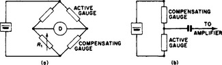
Torque: For a circular-section shaft in torsion, the principal stresses lie at 45° to the axis. If four gauges are applied as in Figure 11.49, and connected to a bridge through suitable slip-ring gear (usually silver ring surfaces and silver graphite brushes), the bridge unbalance is four times that of a single gauge. The arrangement is inherently temperature compensated. For engine testing it is normal to make up a special length of shaft with gauges and slip-rings, to be fitted between the engine and the brake or driven unit. With automatic recorders it is possible to record simultaneous data such as torque, pressure variation, temperature, etc., to give all phenomena on a time base display.
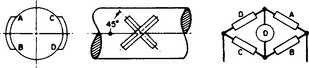
Thrust: Various other measurements of mechanical power transmission can be measured. The arrangement in Figure 11.50 is for thrust. Four axial (A) and four circumferential (C) gauges are disposed symmetrically and connected as indicated in a bridge network, with r as balancing adjustment at zero load. The monitoring system (which can be used with other strain-gauge applications) consists of a self-balancing potentiometer with chart (Ch), digital (Dg) and indicator (Id) readouts. The speed of a self-balancing potentiometer is restricted to about one reading per second.
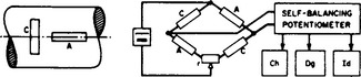
Principal stresses: The direction and magnitude of principal stresses can be determined from a rosette of three or more strain gauges arranged with suitable orientations (Figure 11.51). Commercial rosettes are available in several geometrical formations. As it is unlikely that the principal strain will be on the axis of any one gauge, note must be taken of the sensitivity of the gauges in a direction at right angles to the axis if accurate results are required. The correction is not likely to exceed 3%.
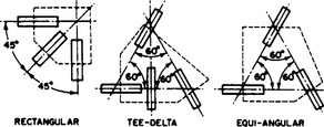
11.12.8 Magnetostrictive transducers
Magnetostriction is the dimensional change that occurs in a ferromagnetic material when subjected to magnetisation, and an inverse effect of change in magnetisation when the physical dimensions are altered by the application of external force. The dimensional changes are very small (e.g. 30 parts in 106), but if the magnetic field alternates at a frequency corresponding to one of the natural frequencies of vibration of the material in some form, such as a bar, resonance increases the vibration amplitude considerably to perhaps 1 part in 103.
Materials vary widely in the magnitude and sign of the magnetostrictive effect, which also depends on the magnetic field intensity. Pure iron may have positive or negative magnetostriction: the addition of nickel makes the effect positive at all frequencies. With 30% Ni the longitudinal magnetostriction falls to zero, a property utilised in invar–nickel alloys to give very low coefficients of thermal expansion, because the latter is neutralised by the magnetostrictive contraction. In nickel alloys there is a peak dimensional change when the Ni content is about 45% and at about 63% the most sensitive magnetostrictive condition is reached.
11.12.8.1 Sensors
For the purpose of detecting surface and submarine ships, magnetostriction transducers have been employed using under-water supersonic vibrations. The compression stresses generated by the transmitter are reflected by the submerged object and are picked up by a detector utilising the inverse effect–-i.e. change of magnetic properties under mechanical stress.
The presence of flaws, air pockets or impurities can similarly be detected in some opaque substances (e.g. rubber) which should normally be homogeneous. The phase displacement between the incident and reflected waves can be interpreted to indicate the position of the obstruction.
Liquid level can be controlled by a sensor probe just above the required level and connected to an oscillator network. As the level of the liquid reaches the probe, the oscillation ceases because of the greatly increased damping. For the measurement of mechanical stress (Figure 11.52) the bridge is balanced when the sensor and compensating elements are equally stressed, the compensating element eliminating thermal errors. If the stress in the sensor element is increased, its permeability is reduced, and the out-of-balance current is indicated on the detector D, which can be calibrated in stress units. If the stress is rapidly varying, D can be replaced by a cathode-ray oscilloscope.
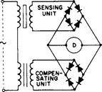
11.12.9 Reactance sensors
Many transducers use the properties of inductive and capacitive reactance. The inductance of an iron-cored inductor varies very rapidly with the length of an included air gap. The basic network in Figure 11.53 employs a bridge with inductors 1 and 2, one with a fixed gap and the other with a gap variable in accordance with some physical quantity such as pressure, strain, thickness, acceleration, etc. The detector D is calibrated appropriately for direct indication. Reliable readings of displacement down to about 3 × 10⁻⁵ mm are readily secured with a properly designed instrument. If the displacement fluctuates, it will modulate the supply waveform, and the modulation waveform can be filtered out from the carrier.
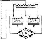
Capacitive reactance can also be used, but as the magnitude of its change with displacement is very small, the capacitor sensor is made to be part of the capacitance in an oscillatory circuit, the frequency of which can be related to the displacement. One type of capacitor pressure sensor consists of two flexible parallel plates with a ‘vacuum’ dielectric. A cylindrical capacitor suitable for sensing high pressures has as electrodes an inner deforming cylinder and an outer ring section: dimensional changes in the radial gap occur when the axial force on the inner cylinder causes a change in its diameter. The change of capacitance is well within the range of commercial straingauge bridges.
11.12.9.1 Angular velocity sensors
Measurements can be read from the output of a permanent-magnet d.c. tachometer for speeds up to 3000 rev/min. The instrument is direct-reading, but a proportional direct output voltage can be used as an electrical transducer. For low speeds the commutator ripple can be excessive and an a.c. tachometer with full-wave rectification will provide a more uniform output, particularly if the instrument is of the multi-tooth variable-reluctance type. These instruments act as loads on the source and they are unable to assess the fine detail of the angular velocity such as superimposed small amplitude oscillations, or non-uniform accelerations and retardations due to changes in load. Simple optical solutions to the problem involve the use of a stroboscope or photosensor coupled with digital counters, and each method avoids any loading of the machine.
11.12.10 Stroboscope
The stroboscope generates high-intensity impulsive flashes of light at controllable repetition frequency. If the repetition frequency corresponds to the time of one revolution of a rotating object or to one complete excursion of a reciprocating object (or any multiple thereof), the object appears to be at rest. If the period is a submultiple 1/n, then the object appears stationary in n different positions. It is desirable for the repetition frequency to exceed 30 Hz in order to avoid visual flicker.
From the flash frequency and observation, the character of velocity perturbations can be viewed and counted and dynamic distortion effects seen. Electrical stroboscopes may involve special neon lamps connected to the secondary side of an induction coil, the primary of which is interrupted by a driven tuning fork. In modern instruments the lamp is a xenon gas discharge tube emitting white light. The flashing frequency is adjusted by means of a transistorised multivibrator-shaper circuit producing pulses of constant energy and fast rise time. Each trigger pulse initiates the discharge of a capacitor to create the flash. Capacitor recharging limits the upper frequency to about 1.5 kHz with a 200 lux illumination level. High frequencies up to 10 kHz can be obtained from a Z-modulated cathode-ray tube as a low-level light source.
11.12.11 Photosensors
In this context, ‘light’ usually means radiation at wavelengths covering the visible spectrum from the near infrared to the near ultraviolet. Light transducers can be identified by three basic forms of physical behaviour: photovoltaic, photoresistive/photojunction and photoemissive.
11.12.11.1 Photovoltaic
Photovoltaic sensors are p—n junction devices with the normal barrier layer potential present between the two materials. When illuminated, the higher-energy protons raise electrons from the valence into the conduction band to create electron–hole pairs. The consequent continual charge separation is enough to drive current through a resistive load without any external source.
Selenium cell: This has a linear current/illumination characteristic for load resistances up to 100Ω, but the relation is progressively more non-linear for higher resistance, and reaches an open-circuit e.m.f. of 0.6 V. The peak spectral response is in the centre of the visible band (0.57 μm), but the energy efficiency is only 0.5%.
Silicon p—n junction cell: The energy conversion is 10–15%, which is adequate for solar cell use in space vehicles. As the time response (a few microseconds) is very fast, silicon photocell arrays are used for reading punched-card and tape, and for optical tracking. The output of a single sensor is typically 70 μA for 5000 lux, the current being constant up to 200 mV. When they are reverse-biased, silicon photosensors behave as photoresistive devices.
11.12.11.2 Photoresistive
A photoresistive sensor consists of a single homogeneous semiconductor material such as n-type cadmium sulphide or cadmium selenide. The material is doped to permit of a large electron charge amplification by the selective absorption of holes, and a spectral response that can simulate that of the eye. This type of sensor is well known as a photographic exposure meter. The CdS sensor is not quite linear over wide illumination ranges, and its response time (100 ms), is slow compared with that (10 ms) of the CdSe type.
The sensors can be used in series with a source and a relay, the latter operating when illumination reduces the sensor resistance to about 1 k Ω. The power dissipation by the sensor can be minimised if the slow resistance changes are used to alter the state of a conventional Schmitt trigger circuit (Figure 11.54). The required illumination level is set by R1; when the illumination is reduced, the cell resistance rises to switch on T1, which causes T2 to switch off and T3 then saturates. The relay operates when the Zener diode conducts at about 12V. The sensor is useful for alarm circuits, street-lighting control and low-rate counting.
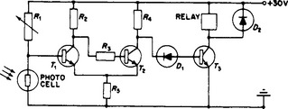
11.12.11.3 Photojunction
Normal diodes and transistors are light-shielded. In the photojunction devices controlled light is admitted to enhance the light effect.
Photodiodes: These are normally of silicon unless the greater infra-red response of germanium is needed. Time constants of 10–100 ns are normal. Silicon planar p-type/intrinsic/n-type photodiodes can respond to laser pulses of 1 ns, and are usable at very low light level equivalent to a current of about 100 pA. Special low-noise transistor amplifiers are required.
Phototransistors: The normal form is the n–p–n silicon planar transistor, with conventional bias except for the reverse-biased photodiode between base and collector. It behaves as a common-collector transistor amplifier with a photocurrent generator between base and collector. The maximum cut-off frequency is 50 kHz. A derivative of the field effect transistor, the ‘photofet’, is more sensitive and the gain–bandwidth product is higher.
11.12.11.4 Photoemissive
Photoemissive sensors are vacuum or gas-filled phototubes. The emission of electrons from the cathode occurs when light falls on it, to be collected by a positive anode. Vacuum phototubes have been superseded for light measurement by photodiodes. In the photomultiplier tube the vacuum emission is enhanced by secondary emission at a succession of anodes to give an electron multiplication of 108 or 109, providing significant output for flashes of very short duration. The photomultiplier is used as a scintillation sensor by viewing the weak light emissions that occur in selected phosphors exposed to α, β or γ radiation. These scintillation ‘counters’ have wide application in spectrophotometry, flying-spot scanning, photon counting and whenever a very weak light signal is to be amplified. An alternative device is the Bendix magnetic multiplier. This consists of a single layer of resistive film with the emissive cathode at one end; by suitable accelerating p.d.s applied along the film, together with shaped magnetic fields, the electrons are multiplied by secondary emission and bounced along the strip to accumulate on an anode to give an overall electron gain of 109. With different emissive materials, ultraviolet rays and X-rays can be amplified for subsequent analysis.
11.12.11.5 Selection
Photovoltaic cells do not require an external supply, but they are generally less sensitive than photoresistive types, which do. Photodiodes can be selected for a range of optimum spectral sensitivities and are fast-operating, particularly so for the silicon planar p–i–n type. Phototransistors provide amplification at the cost of a relatively slow response (minimum 20 μs). Photomultiplier tubes provide high amplification, even for single photons.
Integrated-circuit chips about 4 mm2 in area, produced with progressively more complex networks, can include scores of photodiode arrays, with amplifiers, logic counting networks, scanning circuits, etc., to give such outputs as digital pulse rates proportional to illumination, logic for character recognition and punched-card reading, and as replacements for photomultipliers. These devices find a wide range of application in transducer instrumentation for control and communication.
11.12.12 Nuclear radiation sensors
Radiation sensors are required in particle physics research, for monitoring reactions in nuclear power stations, as gauges for industrial processes, and for measurements employing radioactive isotopes. The emanations used for industrial processes include α, β and γ rays with X-rays for special applications such as the examination of welds; the sensor characteristics largely determine the radiation to be processed. The devices include the following.
Low-pressure gas ionisation chambers to measure α-particles by accumulating the electrons released by their collisions with gas molecules, and without subsequent multiplication.
Proportional counters, similar to the foregoing but with a higher accelerating voltage (500–800 V) to give cumulative gas amplification (Townsend avalanche) and an electron gain of 105–106. The use is for counting α particles in the presence of β particles and γ rays.
Geiger counters operating at 800–1500 V, or at low voltage, for β and γ ray detection. The complete ionisation must be quenched between counts, and the dead time restricts the counting rate to about 1000/s.
Scintillation sensors (or ‘counters’) for α, β or γ detection. There are also semiconductor sensors for the same application and for X-rays.
α, β- and γ-Ray sensors require to be followed by electronic pulse amplifiers and counters. A counter may accumulate a total/fractional scaled count, or it may give a rate-meter display. These outputs, together with pulse height analysers, are used to assess the energy spectra of the received signals. Coincidence counters have multiple input sensors so arranged that only the required type of emanation is measured during any selected period.
The detectors can form the bases for industrial gauges and monitors when used with radioisotope sources. The selective absorption of materials enables β radiations through paper to indicate the uniformity of the product; liquid-level gauges give correcting signals when the rise of level absorbs the radiation; radioisotope tracers with short half-lives can be introduced into liquid and gas channels to indicate flow rate, uniformity of mixing and the detection of leakages.
11.13 Data recording
Chart recorders responsive to signals at frequencies up to a maximum of 25 kHz include: (1) a.c. ultraviolet, (2) X—Y, and (3) analogue and digital strip-chart forms. All provide records of related phenomena that need to be preserved in graphical form.
The visual discrimination of the best-quality trace, when stated as a fraction of the chart width, should not be significantly different from the accuracy and linearity of the display; this condition dictates the width of the chart paper. Many different types of treated chart paper are needed in order to be compatible with the various writing systems mentioned below. Paper is provided in rolls or overlapping folds, the latter being very convenient for quick retrieval of data.
Conventional pens for ink-feed methods use felt, ballpoint or nylon disposable tips. The ink cartridges are easily replaced, and the supply is drawn to the tip by capillary action. The nylon pen is suitable for higher writing speeds; to retain a uniform trace, a variable pressure is automatically applied to the ink cartridge. In multiple-display applications, the possibility of easy trace separation by colour is a unique convenience of ink writing.
Many alternative writing methods have been developed in an attempt to overcome the inertia (response time) limitation of conventional ink writing, as well as to improve the quality of the trace. These include: (a) a heated stylus and sensitive plastic-coated paper; (2) mechanical pressure on chemically treated paper; (3) ultraviolet light beams directed on to photographic paper, the trace appearing and becoming fixed within a few seconds of exposure to natural light; (4) the passage of current through treated metallised paper causing the chemical reduction process to develop a black imprint; and (5) electrostatic copying, in which a flat capacitor is formed from conductive paper with a dielectric coating—a very small area can be charged, and particles are attracted to the charged area to provide the visible trace, which may require treatment to make it permanent.
1. British Standards Institution. BS 5233 Glossary of terms used in metrology. Osaka: Milton Keynes; 1986.
2. Kibble, B.P., Robinson, I.A., Beliss, J.H. Metrologia. 1990;27:173–192.
3. http://www.npl.co.uk/npl/cem/dclf/indexhtml.
4. Galakhova, O.P., Harkness, S., Hermach, F.L., Hirayama, H., Martin, P., Rozdestvenska, T.H., Williams, E.S. IEEE Transactions on Instrumentation and Measurement. 1980;IM-29:396–399.
5. Emmens, T., IEE Electronics and Power. February 1981;166.
6. Jones, L.T., Ressmeyer, J.J., Clark, C.A. Hewlett-Packard Journal. 1981;32(4):23.
7. Ikeda, Y., NPL des Memorandum No 21. 1976.
8. Turgel, R.S., NBS Technical Note No 870. June 1975.
9. Turgel, R.S. IEEE Transactions on Instrumentation and Measurement. 1974;IM-23:337–341.
10. Stockton, J.R. IEE Electronics Letters. 1977;13(14):406–407.
11. Knight, R.B.D., Stockton, J.R., NPL Reports DES60. 1981.