Industrial Instrumentation
Differential pressure flowmeters 12.3.2
Vortex shedding flowmeters 12.3.4
Linear variable differential transformer (LVDT) 12.6.4
Variable capacitance transducers 12.6.6
Velocity and acceleration 12.7
Strain gauges, loadcells and weighing 12.8
12.1 Introduction
Accurate measurement of process variables such as flow, pressure and temperature is an essential part of any industrial process. This chapter describes methods of measuring common process variables.
Like most technologies, instrumentation has a range of common terms with precise meanings.
Measured variable and process variable are both terms for the physical quantity that is to be measured on the plant (e.g. the level in tank 15). The measured value is the actual value in engineering units (e.g. the level is 1252 mm).
A primary element or sensor is the device which converts the measured value into a form suitable for further conversion into an instrumentation signal, i.e. a sensor connects directly to the plant. An orifice plate is a typical sensor. A transducer is a device which converts a signal from one quantity to another (e.g. a PT100 temperature transducer converts a temperature to a resistance). A transmitter is a transducer which gives a standard instrumentation signal (e.g. 4–20 mA) as an output signal, i.e. it converts from the process measured value to a signal which can be used elsewhere.
12.1.2 Range, accuracy and error
The measuring span, measuring interval and range are terms which describe the difference between the lower and upper limits that can be measured, (e.g. a pressure transducer which can measure from 30 to 120 bar has a range of 90 bar). The rangeability or turndown is the ratio between the upper limit and lower limits where the specified accuracy can be obtained. Assuming the accuracy is maintained across the range, the pressure transmitter above has a turndown of 4:1. Orifice plates and other differential flow meters lose accuracy at low flows, and their turndown is less than the theoretical measuring range would imply.
The error is a measurement of the difference between the measured value and the true value. The accuracy is the maximum error which can occur between the process variable and the measured value when the transducer is operating under specified conditions. Error can be expressed in many ways. The commonest are absolute value (e.g.+/−2°C for a temperature measurement), as a percentage of the actual value, or as a percentage of full scale. Errors can occur for several reasons; calibration error, manufacturing tolerances and environmental effects are common.
Many devices have an inherent coarseness in their measuring capabilities. A wire wound potentiometer, for example, can only change its resistance in small steps and digital devices such as encoders inherently measure in discrete steps. The term resolution is used to define the smallest steps in which a reading can be made.
In many applications the accuracy of a measurement is less important than its consistency. The consistency of a measurement is defined by the terms repeatability and hysteresis.
Repeatability is defined as the difference in readings obtained when the same measuring point is approached several times from the same direction.
Hysteresis occurs when the measured value depends on the direction of approach as Figure 12.1. Mechanical backlash or stiction are common causes of hysteresis.

Figure 12.1 Hysteresis, also known as backlash. The output signal is different for an increasing or decreasing input signal
The accuracy of a transducer will be adversely affected by environmental changes, particularly temperature cycling, and will degrade with time. Both of these effects will be seen as a zero shift or a change of sensitivity (known as a span error).
12.1.3 Dynamic effects
A sensor cannot respond instantly to changes in the measured process variable. Commonly the sensor will change as a first order lag as Figure 12.2 and represented by the equation:

Here T is called the time constant. For a step change in input, the output reaches 63% of the final value in time T. Table 12.1 shows the change at later times.
Table 12.1
Response of a first ordere lap to a step input signal
| Time | % Final value |
| T | 63 |
| 2T | 86 |
| 3T | 95 |
| 4T | 98 |
| 5T | 99 |
It follows that a significant delay may occur for a dynamically changing input signal.
A second order response occurs when the transducer is analogous to a mechanical spring/viscous damper. The response of such a system to a step input of height a is given by the second order equation:
where b is the damping factor and ωn the natural frequency. The final steady state value of x is given by:
The step response depends on both b and ωn, the former determining the overshoot and the latter the speed of response as shown on Figure 12.3. For values of b < 1 damped oscillations occur. The case where b = 1 is called critical damping. For b > 1, the system behaves as two first order lags in series.

Figure 12.3 Response of a second order lag to a step Input signal for various values of damping factor
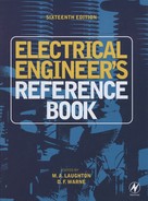
Intuitively one would assume that b = 1 is the ideal value. This may not always be true. If an overshoot to a step input signal can be tolerated a lower value of b will give a faster response and settling time within a specified error band. The signal enters the error band then overshoots to a peak which is just within the error band as shown on Figure 12.4. Many instruments have a damping factor of 0.7 which gives the fastest response time to enter, and stay within, a 5% settling band. Table 12.2 shows optimum damping factors for various settling bands. The settling time is in units of 1/ωn.
Table 12.2
| Settling band | Optimum ‘b’ | Settling time |
| 20% | 0.45 | 1.8 |
| 15% | 0.55 | 2 |
| 10% | 0.6 | 2.3 |
| 5% | 0.7 | 2.8 |
| 2% | 0.8 | 3.5 |
12.1.4 Signals and standards
The signals from most primary sensors are very small and in an inconvenient form for direct processing. Commercial transmitters are designed to give a standard output signal for transmission to control and display devices.
The commonest electrical standard is the 4–20 mA loop. As its name implies this uses a variable current with 4 mA representing one end of the signal range and 20 mA the other. This use of a current (rather than a voltage) gives excellent noise immunity as common mode noise has no effect and errors from different earth potentials around the plant are avoided. Because the signal is transmitted as a current, rather than a voltage, line resistance has no effect.
Several display or control devices can be connected in series provided the total loop resistance does not rise above some value specified for the transducer (typically 250 to 1 k Ω).
Transducers using 4–20 mA can be current sourcing (with their own power supply) as Figure 12.5(a) or designed for two wire operation with the signal line carrying both the supply and the signal as Figure 12.5(b). Many commercial controllers incorporate a 24 V power supply designed specifically for powering two wire transducers.

Figure 12.5 Current loop circuits. (a) Current sourcing with a self powered transducer; (b) Current sinking with a loop powered (two wire) transducer
The use of the offset zero of 4 mA allows many sensor or cable faults to be detected. A cable break or sensor fault will cause the loop current to fall to zero. A cable short circuit will probably cause the loop current to rise above 20 mA. Both of these fault conditions can be easily detected by the display or control device.
12.1.5 P&ID symbols
Instruments and controllers are usually part of a large control system. The system is generally represented by a Piping & Instrumentation drawing (or P&ID) which shows the devices, their locations and the method of interconnection. The description Process & Instrumentation diagram is also used by some sources. The letters P&ID should not be confused with a PID controller described in Chapter 13. The basic symbols and a typical example are shown on Figure 12.6.

The devices are represented by circles called balloons. These contain a unique tag which has two parts. The first is two or more letters describing the function. The second part is a number which uniquely identifies the device, for example FE127 is flow sensor number 127.
The meanings attached to the letters are:
| First letter | Second and subsequent letters | |
| A | Analysis | Alarm (often followed by H for high or L for low) |
| B | Burner | |
| C | Conductivity | Control function |
| D | Density | |
| E | Voltage or misc. electrical | Primary element (sensor) |
| F | Flow | |
| G | Gauging | Glass sight tube (e.g. level) |
| H | Hand | High (with A = alarm) |
| I | Current | Indicator |
| J | Power | |
| K | Time | Control station |
| L | Level | Light. Also Low (with A = alarm) |
| M | Moisture | |
| O | Orifice | |
| P | Pressure | Point |
| Q | Concentration or Quantity | Integration (e.g. flow to volume) |
| R | Radioactivity | Recorder |
| S | Speed | Switch or contact |
| T | Temperature | Parameter to signal conversion |
| U | Multivariable | Multifunction |
| V | Viscosity | Valve |
| W | Weight, force | Well |
| X | Signal to signal conversion | |
| Y | Relay | |
| Z | Position | Drive |
It is good engineering practice for plant devices to have their P&D tag physically attached to them to aid maintenance.
12.2 Temperature
12.2.2 Thermocouples
If two dissimilar metals are joined together as shown in Figure 12.7(a) and one junction is maintained at a high temperature with respect to the other, a current will flow which is a function of the two temperatures. This current, known as the Peltier effect, is the basis of a temperature sensor called a thermocouple. In practice, it is more convenient to measure the voltage difference between the two wires rather than current. The voltage, typically a few mV, is again a function of the temperatures at the meter and the measuring junction.

In practice the meter will be remote from the measuring point. If normal copper cables were used to link the meter and the thermocouple, the temperature of these joints would not be known and further voltages, and hence errors, would be introduced. The thermocouple cables must therefore be run back to the meter. Two forms of cable are used; extension cables which are essentially identical to the thermocouple cable or compensating cables which match the thermocouple characteristics over a limited temperature range. Compensating cables are much cheaper than extension cables.
Because the indication is a function of the temperature at both ends of the cable, correction must be made for the local meter temperature. A common method, called Cold Junction Compensation, measures the local temperature by some other method, (such as a resistance thermometer) and adds in a correction as Figure 12.7(b).
Thermocouples are non-linear devices and the voltage can be represented by an equation of the form:
where a, b, c, d etc. are constants (not necessarily positive) and T is the temperature. Linearising circuits must be provided in the meter if readings are to be taken over an extended range.
Although a thermocouple can be made from any dissimilar metals, common combinations have evolved with well documented characteristics. These are identified by single letter codes. Table 12.3 gives details of common thermocouple types.

Thermocouple tables give the thermocouple voltage at various temperatures when the cold junction is kept at a defined reference temperature, usually 0°C. A typical table for a type K thermocouple is shown on Table 12.4. This has entries in 10°C steps, practical tables are in 1°C steps.
Table 12.4
Voltages for a type K thermocouple, voltages in micro volts with reference junction at 0°C

Thermocouple tables are used in two circumstances: for checking the voltage from a thermocouple with a millivolt-meter or injecting a test voltage from a millivolt source to test an indicator or controller. Because a thermocouple is essentially a differential device with a non-linear response, in each case the ambient temperature must be known. In the examples below the type K thermocouple from Table 12.4 is used.
To interpret the voltage from a thermocouple there are four steps:
(1) Measure the ambient temperature and read the corresponding voltage from the thermocouple table. For an ambient temperature of 20° C and reference voltage of 0°C a type K thermocouple this gives 0.798 mV
(2) Measure the thermocouple voltage. Let us assume it is 12.521 mV
(3) Add the two voltages; 12.521 + 0.798 = 13.319 mV
(4) Read the temperature corresponding to the sum. The thermocouple table shows that the voltage corresponding to 330°C is 13.040 mV and interpolation with 41.9 μV/°C gives a temperature of just over 336°C.
To determine the correct injection voltage there are three steps:
(1) As before measure the ambient temperature at the instrument or controller terminals and read the corresponding voltage from the tables. As before we will assume an ambient of 20°C which gives a voltage of 0.798mV
(2) Find the table voltage corresponding to the required test temperature, say 750° C which gives 31.213 mV
(3) Subtract the ambient voltage from the test temperature voltage. The result of 30.415 mV is the required injection voltage. As before the μV/°C slope can be used to work out voltages for temperatures between the 10°C steps of Table 12.4.
Note that if the local input terminals at the meter are shorted together, the local ambient temperature (from the cold junction compensation) should be displayed. This is a useful quick check.
The tables show that the voltage from a thermocouple is small, typically less than 10 mV. High gain, high stability amplifiers with good common mode rejection are required and care taken in the installation to avoid noise.
In critical applications a high resistance voltage source is connected across the thermocouple so that in the event of a cable break the meter will indicate a high temperature.
12.2.3 Resistance thermometers
If a wire has resistance R0 at 0°C its resistance will increase with increasing temperature giving a resistance Rt at temperature T given by:
where a, b, c etc. are constants. These are not necessarily positive.
This change in resistance can be used to measure temperature. Platinum is widely used because the relationship between resistance and temperature is fairly linear. A standard device is made from a coil of wire with a resistance of 100 Ω at 0°C, giving rise to the common name of a Pt100 sensor. These can be used over the temperature range −200°C to 800°C. At 100°C a Pt100 sensor has a resistance of 138.5 Ω, and the 38.5Ω change from its resistance at 0°C is called the fundamental interval.
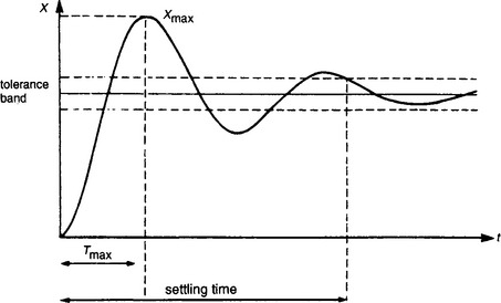
The current through the sensor must be kept low to avoid heating effects. Further errors can be introduced by the resistance of the cabling to the sensor as shown on Figure 12.8(a). Errors from the cabling resistance can be overcome by the use of the three and four wire connections of Figure 12.8(b, c and d). Three wire connections are usually used with a bridge circuit and four wire connections with a constant current source.
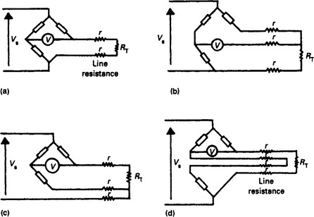
Figure 12.8 The effect of line resistance on RTDs. (a) Simple two wire circuit introduces an error of 2r; (b) Three wire circuit places line resistance into both legs of the measuring bridge; (c) Alternative three wire circuit; (d) Four wire circuit
A thermistor is a more sensitive device. This is a semiconductor crystal whose resistance changes dramatically with temperature. Devices are obtainable which decrease or increase resistance for increasing temperature. The former (decreasing) is more common.
The relationship is very non linear, and is given by:
where R0 is the defined resistance at temperature T0, R the resistance at temperature T and B is a constant called the characteristic temperature. A typical device will go from 300 k Ω at 0°C to 5 k Ω at 100°C.
Although very non-linear, they can be used for measurement over a limited range. Their high sensitivity and low cost makes them very useful for temperature switching circuits where a signal is required if a temperature goes above or below some preset value. Electric motors often have thermistors embedded in the windings to give early warning of motor overload.
12.2.4 Pyrometers
A heated object emits electromagnetic radiation. At temperatures below about 400°C this radiation can be felt as heat. As the temperature rises the object starts to emit visible radiation passing from red through yellow to white as the temperature rises. Intuitively we can use this radiation to qualitatively measure temperature as below:
| Temperature | Colour |
| 500°C | Barely visible dull red glow |
| 800°C | Bright red glow |
| 950°C | Orange |
| 1000°C | Yellow |
| 1200°C | White |
| 1500°C | Dazzling white, eyes naturally avert |
Pyrometers use the same effect to provide a non contact method of measuring temperature.
A pyrometer is, in theory, a very simple device as shown on Figure 12.9. The object whose temperature is to be measured is viewed through a fixed aperture by a temperature measuring device. Part of the radiation emitted by the object falls on the temperature sensor causing its temperature to rise. The object’s temperature is then inferred from the rise in temperature seen by the sensor. The sensor size must be very small, typically of the order of 1mm diameter. Often a circular ring of thermocouples connected in series (called a thermopile) is used. Alternatively a small resistance thermometer (called a bolometer) may be used. Some pyrometers measure the radiation directly using photo-electric detectors.

A major (and surprising) advantage of pyrometers is the temperature measurement is independent of distance from the object provided the field of view is full. As shown on Figure 12.10 the source is radiating energy uniformly in all directions, so the energy received from a point is proportional to the solid angle subtended by the sensor. This will decrease as the square of the distance. There is, however, another effect. As the sensor moves away the scanned area also increases as the square of the distance. These two effects cancel giving a reading which is independent of distance.

Figure 12.10 The effect of object distance on a pyrometer. The energy per unit area decreases with the square of the distance, however the scanned area increases as the square of the distance. Neglecting other influences (such as atmospheric absorption) these effects cancel as the pyrometer reading is independent of distance
Although all pyrometers operate on radiated energy there are various ways in which the temperature can be deduced from the received radiation. The simplest measures the total energy received from the object (which is proportional to T4 where T is the temperature in kelvin). This method is susceptible to errors from lack of knowledge of the emissivity of the object’s surface. This error can be reduced by using filters to restrict the measuring range to frequencies where the object’s emissitivity approaches unity.
An alternative method takes two measurements at two different frequencies (i.e. two different colours) and compares the relative intensities to give an indication of temperature. This method significantly reduces emissivity errors.
Pyrometers have a few major restrictions which should be appreciated. The main problem is they measure surface temperature and only surface temperature. Lack of knowledge of the emissivity is also a major source of error.
12.3 Flow
The term ‘flow’ can generally be applied in three distinct circumstances:
Volumetric flow is the commonest and is used to measure the volume of material passing a point in unit time (e.g. m3 • s−1). It may be indicated at the local temperature and pressure or normalised to some standard conditions using the standard gas law relationship:
where suffix ‘m’ denotes the measured conditions and suffix ‘n’ the normalised condition.
Mass flow is the mass of fluid passing a point in unit time (e.g. kg. s−1).
Velocity of flow is the velocity with which a fluid passes a given point. Care must be taken as the flow velocity may not be the same across a pipe, being lower at the walls. The effect is more marked at low flows.
12.3.2 Differential pressure flowmeters
If a constriction is placed in a pipe as Figure 12.11 the flow must be higher through the restriction to maintain equal mass flow at all points. The energy in a unit mass of fluid has three components:

Figure 12.11 The basis of a differential flow meter. Because the mass flow must be equal at all points (i.e. Q1 = Q2) the flow velocity must increase in the region of A2. As there is no net gain or loss of energy, the pressure must therefore decrease at A2
(1) Kinetic energy given by mv2/2;
(2) Potential energy from the height of the fluid; and
(3) Energy caused by the fluid pressure, called, rather confusingly, flow energy. This is given by P/ρ where P is the pressure and p the density.
In Figure 12.11 the pipe is horizontal, so the potential energy is the same at all points. As the flow velocity increases through the restriction, the kinetic energy will increase and, for conservation of energy, the flow energy (i.e. the pressure) must fall.
This equation is the basis of all differential flow meters.
Flow in a pipe can be smooth (called streamline or laminar) or turbulent. In the former case the flow velocity is not equal across the pipe being lower at the walls. With turbulent flow the flow velocity is equal at all points across a pipe.
For accurate differential measurement the flow must be turbulent.
The flow characteristic is determined by the Reynolds number defined as:
where v is the fluid velocity, D the pipe diameter, ρ the fluid density and η the fluid viscosity. Sometimes the kinematic viscosity ρ/η is used in the formula. The Reynolds number is a ratio and has no dimensions. If Re < 2000 the flow is laminar. If Re > 105 the flow is fully turbulent.
Calculation of the actual pressure drop is complex, especially for compressible gases, but is generally of the form:
where K is a constant for the restriction and ΔP the differential pressure. Methods of calculating K are given in British Standard BS 1042 and ISO 5167:1980. Computer programs can also be purchased.
The commonest differential pressure flow meter is the orifice plate shown on Figure 12.12. This is a plate inserted into the pipe with upstream tapping point at D and downstream tapping point at D/2 where D is the pipe diameter. The plate should be drilled with a small hole to release bubbles (liquid) or drain condensate (gases). An identity tag should be fitted showing the scaling and plant identification.
The D-D/2 tapping is the commonest, but other tappings shown on Figure 12.13 may be used where it is not feasible to drill the pipe.

Figure 12.13 Common methods of mounting orifice plates. (a) D-D/2, probably the commonest; (b) Flange taps used on large pipes with substantial flanges; (c) Corner taps drilled through flange; (d) Plate taps, tappings built into the orifice plate; (e) Orifice carrier, can be factory made and needs no drilling on site; (f) Nozzle, gives smaller head loss
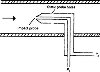
Orifice plates suffer from a loss of pressure on the down stream side (called the head loss). This can be as high as 50%. The venturi tube and Dall tube of Figure 12.14(b) have lower losses of around 5% but are bulky and more expensive. Another low loss device is the pitot tube of Figure 12.15. Equation 12.1 applies to all these devices, the only difference being the value of the constant K.

Figure 12.14 Low loss differential pressure primary sensors. Both give a much lower head loss than an orifice plate but at the expense of a great increase on pipe length. It is often impossible to provide the space for these devices. (a) Venturi tube; (b) Dall Tube
Conversion of the pressure to an electrical signal requires a differential pressure transmitter and a linearising square root unit. This square root extraction is a major limit on the turndown as zeroing errors are magnified. A typical turndown is 4:1.
The transmitter should be mounted with a manifold block as shown on Figure 12.16 to allow maintenance. Valves B and C are isolation valves. Valve A is an equalising valve and is used, along with B and C, to zero the transmitter. In normal operation A is closed and B and C are open. Valve A should always be opened before valves B and C are closed prior to removal of the transducer to avoid high pressure being locked into one leg. Similarly on replacement, valves B and C should both be opened before valve A is closed to prevent damage from the static pressure.

Figure 12.16 Connection of a differential pressure flow sensor such as an orifice plate to a differential pressure transmitter. Valves B and C are used for isolation and valve A for equalisation
Gas measurements are prone to condensate in pipes, and liquid measurements are prone to gas bubbles. To avoid these effects, a gas differential transducer should be mounted above the pipe and a liquid transducer below the pipe with tap off points in the quadrants as shown later in Section 12.4.6.
Although the accuracy and turndown of differential flowmeters is poor (typically 4% and 4:1) their robustness, low cost and ease of installation still makes them the commonest type of flowmeter.
12.3.3 Turbine flowmeters
As its name suggests a turbine flowmeter consists of a small turbine placed in the flow as Figure 12.17. Within a specified flow range, (usually with about a 10:1 turndown for liquids, 20:1 for gases,) the rotational speed is directly proportional to flow velocity.

Figure 12.17 A turbine flow meter. These are vulnerable to bearing failures if the fluid contains any solid particles
The turbine blades are constructed of ferromagnetic material and pass below a variable reluctance transducer producing an output approximating to a sine wave of the form:
where A is a constant, ω is the angular velocity (itself proportional to flow) and N is the number of blades. Both the output amplitude and the frequency are proportional to flow, although the frequency is normally used.
The turndown is determined by frictional effects and the flow at which the output signal becomes unacceptably low. Other non linearities occur from the magnetic and viscous drag on the blades. Errors can occur if the fluid itself is swirling and upstream straightening vanes are recommended.
Turbine flowmeters are relatively expensive and less robust than other flowmeters. They are particularly vulnerable to damage from suspended solids. Their main advantages are a linear output and a good turndown ratio. The pulse output can also be used directly for flow totalisation.
12.3.4 Vortex shedding flowmeters
If a bluff (non-streamlined) body is placed in a flow, vortices detach themselves at regular intervals from the down-stream side as shown on Figure 12.18. The effect can be observed by moving a hand through water. In flow measurement the vortex shedding frequency is usually a few hundred Hz. Surprisingly at Reynolds numbers in excess of 103 the volumetric flow rate, Q, is directly proportional to the observed frequency of vortex shedding f, i.e.

where K is a constant determined by the pipe and obstruction dimensions.
The vortices manifest themselves as sinusoidal pressure changes which can be detected by a sensitive diaphragm on the bluff body or by a downstream modulated ultrasonic beam.
The vortex shedding flowmeter is an attractive device. It can work at low Reynolds numbers, has excellent turndown (typically 15:1), no moving parts and minimal head loss.
12.3.5 Electromagnetic flowmeters
In Figure 12.19(a) a conductor of length l is moving with velocity v perpendicular to a magnetic field of flux density B. By Faraday’s law of electromagnetic induction a voltage E is induced where:

Figure 12.19 Electromagnetic flowmeter. (a) Electromagnetic induction in a wire moving in a magnetic field; (b) The principle applied with a moving conductive fluid
This principle is used in the electromagnetic flowmeter. In figure 12.19(b) a conductive fluid is passing down a pipe with mean velocity v through an insulated pipe section. A magnetic field B is applied perpendicular to the flow. Two electrodes are placed into the pipe sides to form, via the fluid, a moving conductor of length D relative to the field where D is the pipe diameter. From Equation 12.2 a voltage will occur across the electrodes which is proportional to the mean flow velocity across the pipe.
Equation 12.2 and Figure 12.19(b) imply a steady d.c. field. In practice an a.c. field is used to minimise electrolysis and reduce errors from d.c. thermoelectric and electrochemical voltages which are of the same order of magnitude as the induced voltage.
Electromagnetic flowmeters are linear and have an excellent turndown of about 15:1. There is no practical size limit and no head loss. They do, though provide a few installation problems as an insulated pipe section is required, with earth bonding either side of the meter to avoid damage from any welding which may occur in normal service. They can only be used on fluids with a conductivity in excess of 1 mS m−1 which permits use with many, (but not all), common liquids but prohibits their use with gases. They are useful with slurries with a high solids content.
12.3.6 Ultrasonic flowmeters
The Doppler effect occurs when there is relative motion between a sound transmitter and receiver as shown on Figure 12.20(a). If the transmitted frequency is ft Hz, Vs is the velocity of sound and V the relative velocity, the observed received frequency, fr will be:

Figure 12.20 An Ultrasonic Flowmeter. (a) Principle of operation; (b) Schematic of a clip on ultrasonic flowmeter
A Doppler flowmeter injects an ultrasonic sound wave (typically a few hundred kHz) at an angle θ into a fluid moving in a pipe as shown on Figure 12.20(b). A small part of this beam will be reflected back off small bubbles, solid matter, vortices etc. and is picked up by a receiver mounted alongside the transmitter. The frequency is subject to two changes, one as it moves upstream against the flow, and one as it moves back with the flow. The received frequency is thus:
The Doppler flowmeter measures mean flow velocity, is linear, and can be installed (or removed) without the need to break into the pipe. The turndown of about 100:1 is the best of all flowmeters. Assuming the measurement of mean flow velocity is acceptable it can be used at all Reynolds numbers. It is compatible with all fluids and is well suited for difficult applications with corrosive liquids or heavy slurries.
12.3.7 Hot wire anemometer
If fluid passes over a hot object, heat is removed. It can be shown that the power loss is:
where v is the flow velocity and A and B are constant. A is related to radiation and B to conduction.
Figure 12.21 shows a flowmeter based on Equation 12.3. A hot wire is inserted in the flow and maintained at a constant temperature by a self balancing bridge. Changes in the wire temperature result in a resistance change which unbalances the bridge. The bridge voltage is automatically adjusted to restore balance.

The current, I, though the resistor is monitored. With a constant wire temperature the heat dissipated is equal to the power loss from which:
Obviously the relationship is non linear, and correction will need to be made for the fluid temperature which will affect constants A and B.
12.3.8 Mass flowmeters
The volume and density of all materials are temperature dependent. Some applications will require true volumetric measurements, some, such as combustion fuels, will really require mass measurement. Previous sections have measured volumetric flow. This section discusses methods of measuring mass flow.
The relationship between volume and mass depends on both pressure and absolute temperature (measured in kelvin). For a gas:
The relationship for a liquid is more complex, but if the relationship is known and the pressure and temperature are measured along with the delivered volume or volumetric flow the delivered mass or mass flow rate can be easily calculated. Such methods are known as Inferential flowmeters.
In Figure 12.22 a fluid is passed over an in-line heater with the resultant temperature rise being measured by two temperature sensors. If the specific heat of the material is constant, the mass flow, Fm, is given by:

where E is the heat input from the heater, Cp is the specific heat and θ the temperature rise. The method is only suitable for relatively small flow rates.
Many modern mass flowmeters are based on the Coriolis effect. In Figure 12.23 an object of mass m is required to move with linear velocity v from point A to point B on a surface which is rotating with angular velocity. If the object moves in a straight line as viewed by a static observer, it will appear to veer to the right when viewed by an observer on the disc.

If the object is to move in a straight line as seen by an observer on the disc a force must be applied to the object as it moves out. This force is known as the Coriolis force and is given by
where m is the mass, ω is the angular velocity and v the linear velocity. The existence of this force can be easily experienced by trying to move along a radius of a rotating children’s roundabout in a playground.
Coriolis force is not limited to pure angular rotation, but also occurs for sinusoidal motion. This effect is used as the basis of a Coriolis flowmeter shown on Figure 12.24. The flow passes through a ‘C’ shaped tube which is attached to a leaf spring and vibrated sinusoidally by a magnetic forcer. The Coriolis force arises not, as might be first thought, because of the semi-circle pipe section at the right-hand side, but from the angular motion induced into the two horizontal pipe sections with respect to the fixed base. If there is no flow, the two pipe sections will oscillate together. If there is flow, the flow in the top pipe is in the opposite direction to the flow in the bottom pipe and the Coriolis force causes a rolling motion to be induced as shown. The resultant angular deflection is proportional to the mass flow rate.

Figure 12.24 Simple Coriolis mass flowmeter. A multi-turn coil is often used in place of the ‘C’ segment
The original meters used optical sensors to measure the angular deflection. More modern meters use a coil rather than a ‘C’ section and sweep the frequency to determine the resonant frequency. The resonant frequency is then related to the fluid density by:
where K is a constant. The mass flow is determined either by the angular measurement or the phase shift in velocity. Using the resonant frequency maximises the displacement and improves measurement accuracy.
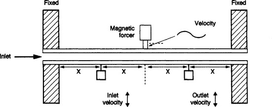
Coriolis measurement is also possible with a straight pipe. In Figure 12.25 the centre of the pipe is being deflected with a sinusoidal displacement, and the velocity of the inlet and outlet pipe sections monitored. The Coriolis effect will cause a phase shift between inlet and outlet velocities. This phase shift is proportional to the mass flow.
12.4 Pressure
There are four types of pressure measurement.
Differential pressure is the difference between two pressures applied to the transducer. These are commonly used for flow measurement as described in Section 12.3.2.
Gauge pressure is made with respect to atmospheric pressure. It can be considered as a differential pressure measurement with the low pressure leg left open. Gauge pressure is usually denoted by the suffix ‘g’ (e.g. 37 psig). Most pressure transducers in hydraulic and pneumatic systems indicate gauge pressure.
Absolute pressure is made with respect to a vacuum.

Atmospheric pressure is approximately 1 bar, 100 kPa or 14.7 psi.
Head pressure is used in liquid level measurement and refers to pressure in terms of the height of a liquid (e.g. inches water gauge). It is effectively a gauge pressure measurement, but if the liquid is held in a vented vessel any changes in atmospheric pressure will affect both legs of the transducer equally giving a reading which is directly related to liquid height.
The head pressure is given by:
where P is the pressure in pascals, ρ is the density (kgm−2), g is acceleration due to gravity (9.8 ms−2) and h the column height in metres.
In Imperial units, pounds are a term of weight (i.e. force) not mass so Equation 12.4 becomes
where P is the pressure in pounds per square unit (inch or foot), ρ the density in pounds per cubic unit and h is the height in units.
12.4.2 Manometers
Although manometers are not widely used in industry they give a useful insight into the principle of pressure measurement. If a U-tube is part filled with liquid, and differing pressures applied to both legs as Figure 12.26, the liquid will fall on the high pressure side and rise on the low pressure side until the head pressure of liquid matches the pressure difference. If the two levels are separated by a height h then

Figure 12.26 The U tube manometer. (a) Pressures P1 and P2 are equal; (b) Pressure P1 is greater than P2 and the distance h is proportional to (P1−P2)
where P1 and P2 are the pressures (in pascals), ρ is the density of the liquid and g is the acceleration due to gravity.
12.4.3 Elastic sensing elements
The Bourdon tube, dating from the mid nineteenth century, is still the commonest pressure indicating device. The tube is manufactured by flattening a circular cross-section tube to the section shown on Figure 12.27 and bending it into a C shape. One end is fixed and connected to the pressure to be measured. The other end is closed and left free.

If pressure is applied to the tube it will try to straighten causing the free end to move up and to the right. This motion is converted to a circular motion for a pointer with a quadrant and pinion linkage. A Bourdon tube inherently measures gauge pressure.
Bourdon tubes are usable up to about 50 MPa, (about 10000 psi). Where an electrical output is required the tube can be coupled to a potentiometer or LVDT.
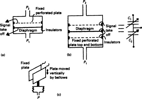
Diaphragms can also be used to convert a pressure differential to a mechanical displacement. Various arrangements are shown on Figure 12.28. The displacement can be measured by LVDTs (see Section 12.6.4), strain gauges (see Section 12.8.3). The diaphragm can also be placed between two perforated plates as Figure 12.29 The diaphragm and the plates form two capacitors whose value is changed by the diaphragm deflection.

12.4.4 Piezo elements
The piezo electric effect occurs in quartz crystals. An electrical charge appears on the faces when a force is applied. This charge is directly proportional to the applied force. The force can be related to pressure with suitable diaphragms. The resulting charge is converted to a voltage by the circuit of Figure 12.30 which is called a charge amplifier. The output voltage is given by:
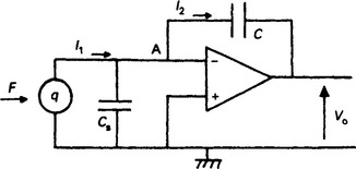
Because q is proportional to the force, V is proportional to the force applied to the crystal. In practice the charge leaks away, even with FET amplifiers and low leakage capacitors. Piezo-electric transducers are thus unsuitable for measuring static pressures, but they have a fast response and are ideal for measuring fast dynamic pressure changes.
A related effect is the piezo resistive effect which results in a change in resistance with applied force. Piezo resistive devices are connected into a Wheatstone bridge.
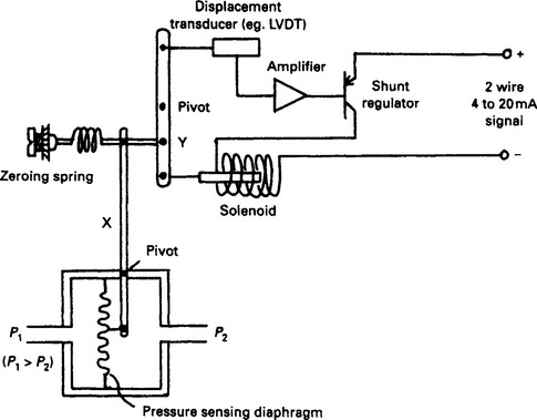
12.4.5 Force balance systems
Friction and non-linear spring constants can cause errors in elastic displacement transducers. The force balance system uses closed loop control to balance the force from the pressure with an opposing force which keeps the diaphragm in a fixed position as shown on Figure 12.31. As the force from the solenoid is proportional to the current, the current in the coil is directly proportional to the applied pressure. LVDTs are commonly used for the position feedback.
12.4.6 Vacuum measurement
Vacuum measurement is normally expressed in terms of the height of a column of mercury which is supported by the vacuum (e.g. mmHg). Atmospheric pressure (approximately 1 bar) thus corresponds to about 760 mmHg, and an absolute vacuum is 0 mmHg. The term ‘torr’ is generally used for 1 mmHg. Atmospheric pressure is thus about 760 torr.
Conventional absolute pressure transducers are usable down to about 20 torr with special diaphragms. At lower pressures other techniques, described below, must be used. At low pressures the range should be considered as logarithmic, i.e. 1 to 0.1 torr is the same ‘range’ as 0.1 torr to 0.01 torr.
The first method, called the Pirani gauge, applies constant energy to heat a thin wire in the vacuum. Heat is lost from a hot body by conduction, convection and radiation. The first two losses are pressure dependent. The heat loss decreases as the pressure falls causing the temperature of the wire to rise. The temperature of the wire can be measured from its resistance (see Section 12.2.3) or by a separate thermocouple.
The range of a Pirani gauge is easily changed by altering the energy supplied to the wire. A typical instrument would cover the range 5 torr to 10−5 torr in three ranges. Care must be taken not to overheat the wire which will cause a change in the heat loss characteristics.
The second technique, called an ionisation gauge, is similar to a thermionic diode. Electrons emitted from the heated cathode cause a current flow which is proportional to the absolute pressure. The current is measured with high sensitivity microammeters. Ionisation gauges can be used over the range 10−3 to 10−12 torr.
12.4.7 Installation notes
To avoid a response with a very long time constant the pipe run between a plant and a pressure transducer must be kept as short as possible. This effect is particularly important with gas pressure transducers which can exhibit time constants of several seconds if the installation is poor.
Entrapped air can cause significant errors in liquid pressure measurement, and similarly condensed liquid will cause errors in gas pressure measurement. Ideally the piping should be taken from the top of the pipe and rise to the transducer for gas systems, and be taken from the lower half of the pipe and fall to the transducer for liquid pressure measurement. If this is not possible, vent/drain cocks must be fitted. Care must be taken to avoid sludge build up around the tapping with liquid pressure measurement. Typical installations are shown on Figure 12.32. Under no circumstances should the piping form traps where gas bubbles or liquid sumps can form.

Figure 12.32 Installation of pressure transducers. Similar considerations apply to differential pressure transducers used with orifice plates and similar primary flow sensors. (a) Gas pressure transducer; (b) Liquid pressure transducer; (c) Faulty installations with potential traps
Steam pressure transducers are a special case. Steam can damage the transducer diaphragm, so the piping leg to the transducer is normally arranged to naturally fill with water by taking the tapping of the top of the pipe and mounting the transducer (with unlagged pipes) below the pipe as Figure 12.33(a). If this is not possible, a steam trap is placed in the piping as Figure 12.33(b).
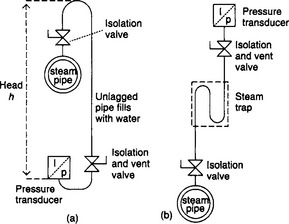
Figure 12.33 Piping arrangements for steam pressure transducers. (a) Preferred arrangement; (b) Alternative arrangement
In both cases there will be an offset from the liquid head. A similar effect occurs when a liquid pressure transmitter is situated below the pipe. In both cases the offset pressure can usually be removed in the transducer setup.
Pressure transducers will inevitably need to be changed or maintained on line, so isolation valves should always be fitted. These should include an automatic vent on closure so pressure cannot be locked into the pipe between the transducer and the isolation valve.
Where a low pressure range differential transducer is used with a high static pressure, care must be taken to avoid damage by the static pressure getting ‘locked in’ to one side. Figure 12.16 (Section 12.3.2) shows a typical manifold for a differential transducer. The bypass valve should always be opened first on removal and closed last on replacement.
12.5 Level transducers
A float is the simplest method of measuring or controlling level. Figure 12.34 shows a typical method of converting the float position to an electrical signal. The response is non linear, with the liquid level being given by:

To minimise errors the float should have a large surface area.
12.5.2 Pressure based systems
The absolute pressure at the bottom of a tank has two components and is given by:
where ρ is the density, g is gravitational acceleration and h the depth of the liquid. The term ρgh is called the head pressure. Most pressure transducers measure gauge pressure, (see Section 12.4.1), so the indicated pressure will be directly related to the liquid depth. It should be noted that ‘h’ is the height difference between the liquid surface and the pressure transducer itself. An offset may need to be added, or subtracted, to the reading as shown on Figure 12.35(a).

Figure 12.35 Level measurement from hydrostatic pressure. (a) Head error arising from transducer position. This error can be removed by a simple offset; (b) Differential pressure measurement in a pressurised tank; (c) Level measurement with condensable liquid. This method is commonly used for drum level in steam boilers
If the tank is pressurised, a differential pressure transmitter must be used as Figure 12.35(b). This arrangement may also require a correction if the pressure transducer height is not the same as the tank bottom. Problems can also occur if condensate can form in the low pressure leg as the condensate will have its own, unknown, head pressure.
In these circumstances the problems can be overcome by deliberately filling both legs with fluid as Figure 12.35(c). Note that the high pressure leg is now connected to the tank top. The differential pressure is now:
where ρ1 is the liquid density and ρ2 the vapour density (often negligible). Note that the equation is independent of the transducer offset H1. This arrangement is often used in boiler applications to measure the level of water in the drum. The filling of the pipes often occurs naturally if they are left unlagged.
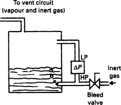
One problem of all methods described so far is that the pressure transducer must come into contact with the fluid. If the fluid is corrosive or at a high temperature this may cause early failures. The food industries must also avoid stagnant liquids in the measuring legs. One solution is the gas bubbler of Figure 12.36. Here an inert gas (usually argon or nitrogen), is bubbled into the liquid, and the measured gas pressure will be the head pressure ρgh at the pipe exit.
12.5.3 Electrical probes
Capacitive probes can be used to measure the depth of liquids and solids. A rod, usually coated with PVC or PTFE, is inserted into the tank (Figure 12.37(a)) and the capacitance measured to the tank wall. This capacitance has two components, C1 above the surface and C2 below the surface. As the level rises C1 will decrease and C2 will increase. These two capacitors are in parallel, but as liquids and solids have a higher di-electric constant than vapour, the net result is that the capacitance rises for increasing level.

Figure 12.37 Level measurement using a capacitive probe. (a) Physical arrangement; (b) A.c. bridge circuit
The effect is small, however, and the change is best measured with an a.c. bridge circuit driven at about 100 kHz (Figure 12.37(b)). The small capacitance also means that the electronics must be close to the tank to prevent errors from cable capacitance.
The response is directly dependent on the dielectric constant of the material. If this changes, caused, say, by bubbling or frothing, errors will be introduced.
If the resistance of a liquid is reasonably constant, the level can be inferred by reading the resistance between two submerged metal probes. Stainless steel is often used to reduce corrosion. A bridge measuring circuit is again used with an a.c. supply to avoid electrolysis and plating effects. Corrosion can be a problem with many liquids, but the technique works well with water. Cheap probes using this principle are available for stop/start level control applications.
12.5.4 Ultrasonic transducers
Ultrasonic methods use high frequency sound produced by the application of a suitable a.c. voltage to a piezo electric crystal. Frequencies in the range 50 kHz to 1 MHz can be used, although the lower end of the range is more common in industry. The principle is shown on Figure 12.38. An ultrasonic pulse is emitted by a transmitter. It reflects off the surface and is detected by a receiver. The time of flight is given by:

where v is the velocity of sound in the medium above the surface. The velocity of sound in air is about 3000 ms−1, so for a tank whose depth can vary from 1 to 10 m, the delay will vary from about 7 ms (full) to 70 ms (empty).
There are two methods used to measure the delay. The simplest, assumed so far and most commonly used in industry, is a narrow pulse. The receiver will see several pulses, one almost immediately through the air, the required surface reflection and spurious reflections from sides, the bottom and rogue objects above the surface (e.g. steps and platforms). The measuring electronics normally provides adjustable Filters and upper and lower limits to reject unwanted readings.
Pulse driven systems lose accuracy when the time of flight is small. For a distance below a few millimetres a swept frequency is used where a peak in the response will be observed when the path difference is a multiple of the wavelength, i.e.
where v is the velocity of propagation and f the frequency at which the peak occurs. Note that this is ambiguous as peaks will also be observed at integer multiples of the wavelength.
Both methods require accurate knowledge of the velocity of propagation. The velocity of sound is 1440 ms−1 in water, 3000 ms−1 in air and 5000 ms−1 in steel. It is also temperature dependent varying in air by 1% for a 30°C temperature change. Pressure also has an effect. If these changes are likely to be significant they can be measured and correction factors applied.
12.5.5 Nucleonic methods
Radioactive isotopes (such as cobalt 60) spontaneously emit gamma or beta radiation. As this radiation passes through the material it is attenuated according to the relationship:
where I0 is the initial intensity, m is a constant for the material, ρ is the density and d the thickness of the material. This equation allows a level measurement system to be constructed in one of the ways shown on Figure 12.39. In each case the intensity of the received radiation is dependent on the level, being a maximum when the level is low.
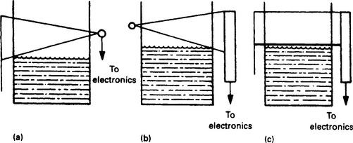
Figure 12.39 Various methods of level measurement using a radio-active source. (a) Line source, point detector; (b) Point source, line detector; (c) Collimated line source, line detector
The methods are particularly attractive for aggressive materials or extreme temperatures and pressures as all the measuring equipment can be placed outside the vessel.
Sources used in industry are invariably sealed, i.e. contained in a lead or similar container with a shuttered window allowing a narrow beam (typically 40° × 7°) to be emitted. The window can usually be closed when the system is not in use and to allow safe transportation. Source strength is determined by the number of disintegrations per second (dps) at the source. There are two units in common use; the curie, (Ci 3.7 × 10¹⁰ dps) and the SI derived unit the bequerel (Bq 1 dps). The typical industrial source would be 500 mCi (18.5 GBq) caesium 137 although there are variations by a factor of at least ten dependent on the application.
The strength of a source decays exponentially with time and this decay is described by the half life which is the time taken for the strength to decrease by 50%. Cobalt 60, a typical industrial source, for example has a half life of 3.5 years and will hence change by about 1% per month. Sources thus have a built in drift and a system will require regular calibration.
The biological effects of radiation are complex and there is no real safe level; all exposure must be considered harmful and legislation is based around the concept of ALARP; ‘as low as reasonably practical’. Exposures should be kept as low as possible, and figures quoted later should not be considered as design targets.
The adsorbed dose (AD) is a measure of the energy density adsorbed. Two units are again used; the rad and the SI derived unit the gray. These are more commonly encountered as the millirad (mrad) and the milligray (mGy):

The adsorbed dose is not however directly related to biological damage as it ignores the differing effect of α, β and γ radiation. A quality factor Q is defined which allows a dose equivalent (DE) to be calculated from:
There are, yet again, two units in common use; the rem and SI derived unit the sievert, again these are more commonly encountered as the millirem and millisievert (mSv);
The so called dose rate is expressed as DE/time (e.g. mrem/hr). Dose rates fall off as the inverse square of the distance, i.e. doubling the distance from the source gives one quarter of the dose rate.
British legislation recognises three groups of people:
Classified workers are trained individuals wearing radiation monitoring devices (usually film badges). They must not be exposed to dose rates of more than 2.5 mrem/hr and their maximum annual exposure (DE) is 5 rem. Medical records and dose history must be kept.
Supervised workers operate under the supervision of classified workers. Their maximum dose rate is 0.75 mrem/hr and maximum annual exposure is 1.5 rem.
Unclassified workers refers to others and the general public. Here the dose rate must not exceed 0.25 mrem/hr and the annual exposure must be below 0.5 rem.
It must be emphasised that the principle of ALARP applies and these are not design criteria.
Nucleonic level detection also requires detectors. Two types are commonly used, the Geiger-Muller (GM) tube and the scintillation counter. Both produce a semi-random pulse stream, the number of pulses received in a given time being dependent on the strength of the radiation. This pulse chain must be converted to a d.c. voltage by suitable filtering to give a signal which is dependent on the level of material between the source and the detector.
Conceptually nucleonic level measurement is simple and reliable. Public mistrust and the complex legislation can, however, make it a minefield for the unwary. Professional advice should always be taken before implementing a system.
12.5.6 Level switches
Many applications do not require analogue measurement but just a simple material present/absent signal. For liquids the simplest is a float which hangs down when out of a liquid and inverts when floating. The float orientation is sensed by two internal probes and a small mercury pool. Solids can be detected by rotating paddles or vibrating reeds which seize solid when submerged.
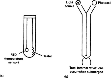
Two non-moving detectors are shown on Figure 12.40. The first is a heated tube whose heat loss will be higher (and hence the sensed temperature lower) when submerged. The second is a light reflective probe which will experience total internal reflection when submerged.
12.6 Position transducers
The measurement of position or distance is of fundamental importance in many applications. It also appears as an intermediate variable in other measurement transducers where the measured variable (such as pressure or force) is converted to a displacement.
12.6.2 The potentiometer
The simplest position transducer is the humble potentiometer. They can directly measure angular or linear displacements. Figure 12.41 shows a potentiometer with track resistance R, connected to a supply Vi and a load RL. If the span is D and the slider at position d, we can define a fractional displacement x = d/D. The output voltage is then:

The error is zero at both ends of the travel and maximum at x = 2/3. If RL is significantly larger than R, the error is approximately 25 · R/RL % of value or 15 · R/RL % of full scale. A 10 K potentiometer connected to a 100 K load will thus have an error of about 1.5% FSD. If RL ![]() R, then V0 = x · Vi.
R, then V0 = x · Vi.
Loading errors are further augmented by linearity and resolution errors. Potentiometers have finite resolution from the wire size or grain size of the track. They are also mechanical devices which require a force to move and hence can suffer from stiction, backlash and hysteresis.
The failure mode of a potentiometer also needs consideration. A track break can cause the output signal to be fully high above the failure point and fully low below it. In closed loop position control systems this manifests itself as a high speed dither around the break point.
Potentiometers can be manufactured with track resistance to give a specified non-linear response (e.g. trigonometric, logarithmic, square root etc.).
12.6.3 Synchros and resolvers
Figure 12.42(a) shows a transformer whose secondary can be rotated with respect to the primary. At angle θ the output voltage will be given by

where K is a constant. This relationship is shown on Figure 12.42(b). The output amplitude is dependent on the angle, and the signal can be in phase (from θ = 270° to 90°) or antiphase (from θ = 90° to 270°). This principle is the basis of synchros and resolvers.
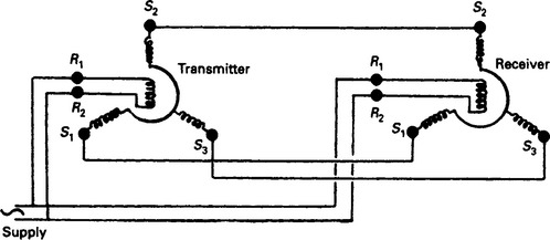
A synchro link in its simplest form consists of a transmitter and receiver connected as Figure 12.43. Although this looks superficially like a three-phase circuit it is fed from a single-phase supply, often at 400 Hz. The voltage applied to the transmitter induces in-phase/anti-phase voltages in the windings as described above and causes currents to flow through the stator windings at the receiver. These currents produce a magnetic field at the receiver which aligns with the angle of the transmitter rotor.
The receiver rotor also produces a magnetic field. If the two receiver fields do not align, torque will be produced on the receiver shaft which causes the rotor to rotate until the rotor and stator fields align, i.e. the receiver rotor is at the same position as the transmitter rotor.
Such a link is called a torque link and can be used to remotely position an indicator. A more useful circuit, shown on Figure 12.44 can be used to give an electrical signal which represents the difference in angle of the two shafts. The receiving device is called a control transformer.

Figure 12.44 Connection of a position control system using a control transformer. The output voltage is zero when the rotor on the control transformer is at 90° to the rotor on the transmitter. Note there are two zero positions 180° apart
The transmitter operates as described above and induces a magnetic field in the control transformer. An a.c. voltage will be induced in the control transformer’s rotor if it is not perpendicular to the field. The magnitude of this voltage is related to the angle error and the phase to the direction.
The a.c. output signal must be converted to d.c. by a phase sensitive rectifier. The Cowan rectifier (Figure 12.45) is commonly used. Another common circuit is the positive/negative amplifier (Figure 12.46) with the electronic polarity switch driven by the reference supply.

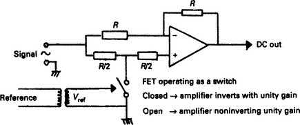
Figure 12.46 Full wave phase sensitive rectifier based on an operational amplifier. The switch represents a FET driven by a reference signal
Resolvers have two stator coils at right angles and a rotor coil as shown on Figure 12.47. The voltages induced in the two stator coils are simply
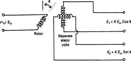
Figure 12.47 The resolver; the reference voltage is applied to the rotor and the output signals read from the two stator windings

Resolvers are used for co-ordinate conversion and conversion from rectangular to polar co-ordinates. They are also widely used with solid state digital converters which give a binary output signal (typically 12 bit). One useful feature is that ![]() is a constant which makes an open circuit winding easy to detect.
is a constant which makes an open circuit winding easy to detect.
Resolvers can also be used with a.c. applied to the stator windings and the output signal taken from the rotor (Figure 12.48). One stator signal is shifted by 90°. Both signals are usually obtained from a pre-manufactured quadrature oscillator. The output signal is then

Figure 12.48 Alternative connection for a resolver. Two reference voltages shifted by 90° are applied to the stator windings and the output read from the rotor. The output signal is a constant amplitude sine wave with phase shift determined by the rotor angle
This a.c. signal can be converted to d.c. by a phase sensitive rectifier.
Complete rotary transducers comprising quadrature oscillator, resolver and phase sensitive rectifier can be obtained which give a d.c. output signal proportional to shaft angle. Because there is little friction these are low torque devices.
12.6.4 Linear variable differential transformer (LVDT)
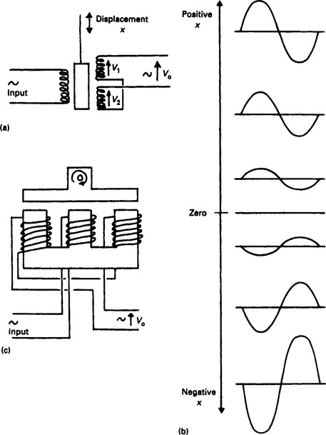
An LVDT is used to measure small displacements, typically less than a few mm. It consists of a transformer with two secondary windings and a movable core as shown on Figure 12.49(a). At the centre position the voltages induced in the secondary windings are equal but of opposite phase giving zero output signal. As the core moves away from the centre one induced voltage will be larger, giving a signal whose amplitude is proportional to the displacement and whose phase shows the direction as Figure 12.49(b). Again a d.c. output signal can be obtained with a phase sensitive rectifier. Figure 12.49(c) shows the same idea used to produce a small displacement angular transducer.
12.6.5 Shaft encoders
Shaft encoders give a digital representation of an angular position. They exist in two forms.
An absolute encoder gives a parallel output signal, typically 12 bits (one part in 4095) per revolution. Binary coded decimal (BCD) outputs are also available. A simplified four bit encoder would therefore operate as in Figure 12.50(a). Most absolute encoders use a coded wheel similar to Figure 12.50(b) moving in front of a set of photocells.

Figure 12.50 Absolute position shaft encoder. (a) Output from a four bit encoder. Real devices use 12 bits and employ unit distance coding such as the Gray code; (b) The wheel on a four bit encoder.
A simple binary coded shaft encoder can give anomalous readings as the outputs change state. Suppose a four bit encoder is going from 0111 to 1000. It is unlikely that all photocells will change together, so the output states could go 0111 > 0000 > 1000 or 0111 > 1111 > 1000 or any other sequence of bits.
There are two solutions to this problem. The first uses an additional track, called an anti-ambiguity track, which is used by the encoder’s internal logic to inhibit changes around transition points.
The second solution uses a unit distance code, such as the Gray code described in Section 14.6.4 which has no ambiguity. The conversion logic from Gray to binary is usually contained within the encoder itself.
Incremental encoders give a pulse output with each pulse representing a fixed distance. These pulses are counted by an external counter to give indication of position. Simple encoders can be made by reading the output from a proximity detector in front of a toothed wheel.
A single pulse output train carries no information as to direction. Commercial incremental encoders usually provide two outputs shifted 90° in phase as Figure 12.51(a). For clockwise rotation, A will lead B as Figure 12.51(b) and the positive edge of A will occur when B is low. For anti-clockwise rotation B will lead A as Figure 12.51(c) and the positive edge of A will occur when B is high. The logic (A and not B) can be used to count up, and (A and B) to count down. The two output incremental encoder can thus be used to follow reversals without cumulative error, but can still lose its datum position after a power failure.
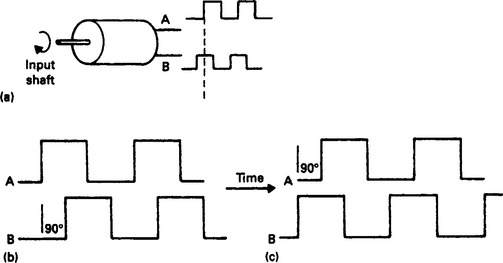
Figure 12.51 The incremental encoder. (a) Physical arrangements—the two phase shifted outputs give directional information; (b) Clockwise rotation; (c) Anti-clockwise rotation
Most PLC systems have dedicated high speed counter cards which can read directly from a two channel incremental encoder.
12.6.6 Variable capacitance transducers
The small deflections obtained in weigh systems or pressure transducers are often converted into an electrical signal by varying the capacitance between two plates. Very small displacements can be detected by these methods.
The capacitance C of a parallel plate capacitor is given by:
where ε is the permitivity of the material between the plates, A the area and d the separation.
Variation in capacitance can be obtained from varying e (sliding in a dielectric, or moving the plates horizontally (change A) or apart (change d)). Although the change is linear for e and A, the effect is small. A common arrangement uses a movable plate between two fixed plates as Figure 12.52(a). Here two capacitors are formed which can be directly connected into an a.c. bridge as Figure 12.52(b). If the fixed plates are distance D apart, d is the null position separation and the centre plate is displaced by x, the output voltage change can be shown to be:

12.6.7 Laser distance measurement
Lasers can give very accurate measurement of distance and are often used in surveying. There are two broad classes of laser distance measurement.
In the first, shown on Figure 12.53 and called a triangulation laser, a laser beam is used to produce a very bright spot on the target object. This is viewed by an imaging device which can be considered as a linear array of tiny photocells. The position of the spot on the image will vary according to the distance as shown, and the distance found by simple triangulation trigonometry.

The second type of distance measurement is used at longer distances and times how long it takes a laser pulse to reach the target and be reflected back. For very long distances, (in surveying for example), a pulse is simply timed. At shorter distances a continuous amplitude modulated laser beam is sent and the phase shift between transmitted and received signals used to calculate the distance. This latter method can give ambiguous results, so often the two techniques are combined to give a coarse measurement from time of flight which is fine tuned by the phase shift.
Lasers can blind, and are classified according to their strength. Class 1 lasers are inherently safe. Class 2 lasers can cause retinal damage with continuous viewing but the natural reaction to blink or look away gives some protection. Class 3 lasers can cause damage before the natural reaction occurs. Risk assessments, safe working practices and suitable guarding must be provided for Class 2 and 3 lasers. Optical devices such as binoculars must never be used whilst working around lasers.
12.6.8 Proximity switches and photocells
Mechanical limit switches are often used to indicate the positional state of mechanical systems. These devices are bulky, expensive and prone to failure where the environment is hostile (e.g. dust, moisture, vibration, heat).
Proximity switches can be considered to be solid state limit switches. The commonest type is constructed around a coil whose inductance changes in the presence of a metal surface. Simple two wire a.c. devices act just like a switch, having low impedance and capable of passing several hundred mA when covered by metal, and a high impedance (typical leakage 1 mA) when uncovered. Sensing distances up to 20 mm are feasible, but 5–10 mm is more common.
The leakage in the off state (typically 1 mA) can cause problems with circuits such as high impedance PLC input cards. In these circumstances a dummy load must be provided in parallel with the input.
D.c. powered switches use three wires, two for the supply and one for the output. D.c. sensors use an internal high frequency oscillator to detect the inductance change which gives a much faster response. Operation at several kHz is easily achieved.
A d.c. proximity detector can have an output in either of the two forms of Figure 12.54. A PNP output switches a positive supply to a load with a return connected to the negative supply. A PNP output is sometimes called a current sourcing output. With an NPN output the load is connected to the positive supply and the proximity detector connects the load to the negative supply. NPN outputs are therefore sometimes called a current sinking output. It is obviously important to match the detector to the load connection.

Figure 12.54 Current sourcing and sinking proximity detectors. (a) PNP current sourcing; (b) NPN current sinking
Inductive detectors only work with metal targets. Capacitive proximity detectors work on the change in capacitance caused by the target and accordingly work with wood, plastic, paper and other common materials. Their one disadvantage is they need adjustable sensitivity to cope with different applications.
Ultrasonic sensors can also be used, operating on the same principle as the level sensor described in Section 12.5.4. Ultrasonic proximity detectors often have adjustable near and far limits so a sensing window can be set.
Photocells (or PECs) are another possible solution. The presence of an object can be detected either by the breaking of a light beam between a light source and a PEC or by bouncing a light beam off the object which is detected by the PEC. In the first approach the PEC sees no light for an object present. In the second approach (called a retro-reflective PEC) light is seen for an object present. It is usual to use a modulated light source to avoid erratic operation with changes in ambient light and prevent interaction between adjacent PECs.
12.7 Velocity and acceleration
Velocity is the rate of change of position, and acceleration is the rate of change of velocity. Conversion between them can therefore be easily achieved by the use of integration and differentiation circuits based on d.c. amplifiers. Integration circuits can, though, be prone to long term drift.
12.7.2 Velocity
Many applications require the measurement of angular velocity. The commonest method is the tachogenerator which is a simple d.c. generator whose output voltage is proportional to speed. A common standard is 10 volts per 1000 rpm. Speeds up to 10 000 rpm can be measured, the upper limit being centrifugal force on the tacho commutator.
Pulse tachometers are also becoming common. These are essentially identical to incremental encoders described in Section 12.6.5 and produce a constant amplitude pulse train whose frequency is directly related to rotational speed. This pulse train can be converted into a voltage in three ways.
The first, basically analog, method used fires a fixed width monostable as Figure 12.55 which gives a mark/space ratio which is speed dependent. The monostable output is then passed through a low pass filter to give an output proportional to speed. The maximum achievable speed is determined by the monostable pulse width.

Figure 12.55 Speed measurement using incremental pulse encoder. The pulses from the encoder fire a fixed duration monostable. The resulting pulse train is filtered to give a mean voltage proportional to speed
The second, digital, method counts the number of pulses in a given time. This effectively averages the speed over the count period which is chosen to give a reasonable balance between resolution and speed of response.
Counting over a fixed time is not suitable for slow speeds as adequate resolution can only be obtained with a long duration sample time. At slow speeds, therefore, the period of the pulses is often directly timed giving an average speed per pulse. The time is obviously inversely proportional to speed.
Digital speed control systems often use both of the last two methods and switch between them according to the speed.
Linear velocity can be measured using Doppler shift. This occurs when there is relative motion between a source of sound (or electromagnetic radiation) and an object. It is commonly experienced as a change of pitch of a car horn as the vehicle passes.
Suppose an observer is moving with velocity v towards a source emitting sound with a frequency f. The observer will see each wavefront arrive early and the perceived frequency will be
where c is the velocity of propagation. As the original frequency is c/l, the frequency shift is
The Doppler shift thus allows remote measurement of velocity. The principle is shown on Figure 12.56. A transmitter, (ultrasonic, radar or light,) emits a constant frequency signal. This is bounced off the target. Two Doppler shifts occur as the object is acting as both moving observer and moving (reflected) source. The frequency shift is thus twice that for the simple case of Equation 12.5.

The transmitted and received frequencies are mixed to give a beat frequency equal to the frequency shift and hence proportional to the target object’s speed. The beat frequency can be measured by counting the number of cycles in a given time.
12.7.3 Accelerometers and vibration transducers
Both accelerometers and vibration transducers consist of a seismic mass linked to a spring as Figure 12.57(a). The movement will be damped by the dashpot giving a second order response defined by the natural frequency and the damping factor, typically chosen to be 0.7.

Figure 12.57 Principle of operation of accelerometers and vibration transducers. (a) Schematic diagram; (b) Frequency response. In region A the device acts as an accelerometer. In region C the device acts as a vibration transducer
If the frame of the transducer is moved sinsusoidally, the relationship between the mass displacement and the frequency will be as Figure 12.57(b).
In region A, the device acts as an accelerometer and the mass displacement is proportional to the acceleration. In region C, the mass does not move, and the displacement with respect to the frame is solely dependent on the frame movement (but is shifted by 180°). In this region the device acts as a vibration transducer. Typically region A extends to about one third of the natural frequency and region C starts at about three times the natural frequency.
In both cases the displacement is converted to an electrical signal by LVDTs or strain gauges.
12.8 Strain gauges, loadcells and weighing
Accurate measurement of weight is required in many industrial processes. There are two basic techniques in use. In the first, shown in Figure 12.58(a) and called a force balance system, the weight of the object is opposed by some known force which will equal the weight. Kitchen scales where weights are added to one pan to balance the object in the other pan use the force balance system. Industrial systems use hydraulic or pneumatic pressure to balance the load, the pressure required being directly proportional to the weight.
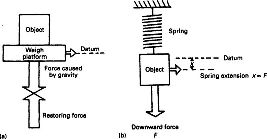
The second, and commoner, method is called strain weighing, and uses the gravitational force from the load to cause a change in the structure which can be measured. The simplest form is the spring balance of Figure 12.58(b) where the deflection is proportional to the load.
12.8.2 Stress and strain
The application of a force to an object will result in deformation of the object. In Figure 12.59 a tensile force F has been applied to a rod of cross-sectional area A and length L. This results in an increase in length ΔL. The effect of the force will depend on the force and the area over which it is applied. This is called the stress, and is the force per unit area:

Stress has the units of N/m2 (i.e. the same as pressure, so pascals are sometimes used).
The resulting deformation is called the strain, and is defined as the fractional change in length.
Strain is dimensionless. Because the change in length is small, microstrain (μstrain defined as strain* 106) is often used. A 10 m rod exhibiting a change in length of 0.0045 mm because of an applied force is exhibiting 45 μstrain.
The strain will increase as the stress increases as shown on Figure 12.60. Over region AB the object behaves as a spring; the relationship is linear and there is no hysteresis (i.e. the object returns to its original dimension when the force is removed. Beyond Point B the object suffers deformation and the change is not reversible. The relationship is now non linear, and with increasing stress the object fractures at point C. The region AB, called the elastic region, is used for strain measurement. Point B is called the elastic limit. Typically AB will cover a range of 10000 μstrain.

The inverse slope of the line AB is sometimes called the elastic modulus (or modulus of elasticity). It is more commonly known as Young’s modulus defined as
Young’s modulus has dimensions of Nm−2, i.e. the same as pressure. It is commonly given in pascals. Typical values are:

When an object experiences strain, it displays not only a change in length but also a change in cross-sectional area. This is defined by Poisson’s ratio, denoted by the Greek letter v. If an object has a length L and width W in its unstrained state and experiences changes ΔL and ΔW when strained, Poisson’s ratio is defined as:
Typically v is between 0.2 and 0.4. Poisson’s ratio can be used to calculate the change in cross-sectional area.
12.8.3 Strain gauges
The electrical resistance of a conductor is proportional to the length and inversely proportional to the cross-section. i.e.
where ρ is a constant called the resistivity of the material.
When a conductor suffers stress, its length and area will both change resulting in a change in resistance. For tensile stress, the length will increase and the cross-sectional area decrease both resulting in increased resistance. Similarly the resistance will decrease for compressive stress.
Ignoring second order effects the change in resistance is given by:
where G is a constant called the gauge factor. ΔL/L is the strain, E, so Equation 12.6 can be re-written:
where E is the strain experienced by the conductor.
Devices based on the change of resistance with load are called strain gauges, and Equation 12.7 is the fundamental strain gauge equation.
Practical strain gauges are not a slab of material as implied so far but consist of a thin small, (typically a few mm), foil similar to Figure 12.61 with a pattern to increase the conductor length and hence the gauge factor. The gauge is attached to some sturdy stressed member with epoxy resin and experiences the same strain as the member. Early gauges were constructed from thin wire but modern gauges are photo-etched from metallised film deposited onto a polyester or plastic backing. Normal gauges can experience up to 10 000 μstrain without damage. Typically the design will aim for 2000 μstrain under maximum load.

A typical strain gauge will have a gauge factor of 2, a resistance of 120Ω and experience 1000 μstrain. From Equation 12.7 this will result in a resistance change of 0.24 Ω.
Strain gauges must ignore strains in unwanted directions. A gauge has two axis, an active axis along which the strain is applied and a passive axis (usually at 90°) along which the gauge is least sensitive. The relationship between these is defined by the cross-sensitivity:
12.8.4 Bridge circuits
The small change in resistance is superimposed on the large unstrained resistance. Typically the change will be 1 part in 5000. In Figure 12.62 the strain gauge Rg is connected into a classical Wheatstone bridge. In the normal laboratory method, Ra and Rb are made equal and calibrated resistance box Rc adjusted until V0, (measured by a sensitive millivolt-meter,) is zero. Resistance Rc then equals Rg.

With a strain gauge, however, we are not interested in the actual resistance, but the change caused by the applied load. Suppose Rb and Rc are made equal, and Ra is made equal to the unloaded resistance of the strain gauge. Voltages V1 and V2 will both be half the supply voltage and V0 will be zero. If a load is applied to the strain gauge such that its resistance changes by fractional change x (i.e. x = ΔR/R) it can be shown that
In a normal circuit x will be very small compared with 2. For the earlier example x has the value 0.24/120 = 0.002, so Equation 12.8 can be simplified to:
But ΔR = E · G · R where E is the strain and G the gauge factor giving
For small values of x, the output voltage is thus linearly related to the strain.
It is instructive to put typical values into Equation 12.9. For a 24 V supply, 1000 μstrain and gauge factor 2 we get 12 mV. This output voltage must be amplified before it can be used. Care must be taken to avoid common mode noise so the differential amplifier circuit of Figure 12.63 is commonly used.
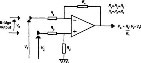
Figure 12.63 Differential amplifier. The output voltage is determined by the difference between the two input voltages
The effect of temperature on resistance was described in Section 12.2.3. and resistance changes from temperature variation are of a similar magnitude to resistance changes from strain. The simplest way of preventing this is to use two gauges arranged as Figure 12.64(a). One gauge has its active axis and the other gauge the passive axis aligned with the load. If these are connected into a bridge circuit as shown on Figure 12.64(b) both gauges will exhibit the same resistance change from temperature and these will cancel leaving the output voltage purely dependent on the strain.

Figure 12.64 Use of multiple strain gauges. (a) Two gauges used to give temperature compensation; (b) Two gauges connected into bridge. Temperature effects will affect both gauges equally and have no effect; (c) Four gauge bridge gives increased sensitivity and temperature compensation; (d) Arrangement for four gauges. Two will be in compression and two in tension for load changes. Temperature affects all gauges equally
Temperature errors can also occur from dimensional changes in the member to which the strain gauges are attached. Gauges are often temperature compensated by having coefficients of linear expansion identical to the material to which they are attached.
Many applications use gauges in all four arms of the bridge as shown on Figure 12.64(c) with two active gauges and two passive gauges. This provides temperature compensation and doubles the output voltage giving
In the arrangement of Figure 12.64(d) four gauges are used with two gauges experiencing compressive strain and two experiencing tensile strain. Here all four gauges are active, giving
Again temperature compensation occurs because all gauges are at the same temperature.
Gauges are manufactured to a tolerance of about 0.5%, i.e. about +/-0.6Ω for a typical 120Ω gauge. As this is larger than the resistance change from strain some form of zeroing will be required. Three methods of achieving this are shown on Figure 12.65. Arrangement b and c are preferred if the zeroing is remote from the bridge.

Figure 12.65 Common methods of bridge balancing. (a) Single leg balancing. R1 is less than R2; (b) Apex balancing; (c) Parallel balancing
Equation 12.10 shows that the output voltage is directly related to the supply voltage. This implies that a large voltage should be used to increase the sensitivity. Unfortunately a high voltage supply cannot be used or I2R heating in the gauges will cause errors and ultimately failure. Bridge voltages of 15–30 V and currents of 20–100 mA are typically used.
Equation 12.10 also implies that the supply voltage must be stable. If the bridge is remote from the supply and electronics, as is usually the case, voltage drops down the cabling can introduce significant errors. Figure 12.66 shows a typical cabling scheme used to give remote zeroing and compensation for cabling resistance. The supply is provided on cores 2 and 6 and monitored on cores 1 and 7 to keep constant voltage at the bridge itself.

12.8.5 Load cells
A loadcell converts a force (usually the gravitational force from an object being weighed) to a strain which can then be converted to an electrical signal by strain gauges. A load cell will typically have the local circuit of Figure 12.67 with four gauges, two in compression and two in tension, and six external connections. The span and zero adjust on test (AOT) are factory set to ensure the bridge is within limits that can be further adjusted on site. The temperature compensation resistors compensate for changes in Young’s modulus with temperature, not changes of the gauges themselves which the bridge inherently ignores.

Figure 12.67 Connection diagram for a typical commercial load cell. Note that a six core cable is required
Coupling of the load requires care, a typical arrangement being shown on Figure 12.68. A pressure plate applies the load to the proof-ring via a knuckle and avoids error from slight misalignment. A flexible diaphragm seals against dust and weather. A small gap ensures that shock overloads will make the loadcell bottom out without damage to the proof-ring or gauges. Maintenance must ensure that dust does not close this gap and cause the proof-ring to carry only part of the load. Bridging and binding are common causes of loadcells reading below the load weight.
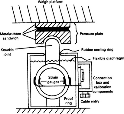
Multi-cell weighing systems can be used, with the readings from each cell being summed electronically. Three cell systems inherently spread the load across all cells. With four cell systems the support structure must ensure that all cells are in contact with the load at all times.
Usually the load cells are the only route to ground from the weigh platform. It is advisable to provide a flexible earth strap, not only for electrical safety but also to provide a route for any welding current which might arise from repairs or later modification.
12.8.6 Weighing systems
A weigh system is usually more than a collection of loadcells and a display. Figure 12.69 is a taring weigh system used when a ‘recipe’ of several materials is to be collected in a hopper. The gross weight is the weight from the load cells, i.e. the materials and the hopper itself. Each time the tare command is given, the gross weight is stored and this stored value subtracted from the gross weight to give the net weight display. In this way the weight of each new material can be clearly seen. This type of weigh system can obviously be linked into a supervisory PLC or computer control network.

Figure 12.70 is a batch feeder system where material is fed from a vibrating feeder into a weigh hopper. The system is first tared, then a two speed system used with a changeover from fast to dribble feed a pre-set weight before the target weight. The feeder turns off just before the correct weight to allow for the material in flight from the feeder. This is known as ‘in flight compensation’, ‘anticipation’ or ‘preact’. To reduce the weigh time the fast feed should be set as fast as possible without causing avalanching in the feed hopper and the changeover to slow feed made as late as possible. The accuracy of the system is mainly dependent on the repeatability of the preact weight, so the slow speed should be set as low as possible.
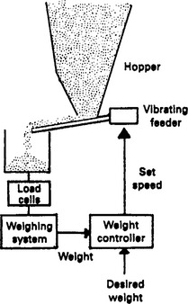
Material is often carried on conveyor belts and Figure 12.71 shows a method of providing feed rate in weight per unit time (e.g. kg per min).
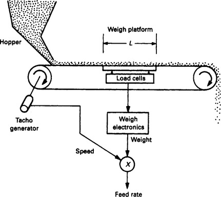
The conveyor passes over a load cell of known length and the linear speed is obtained from the drive motor, probably from a tacho-generator. If the weigh platform has length L m, and is indicating weight W kg at speed V ms−1, the feed rate is simply W · V/L kgs−1.
12.9 Fieldbus systems
A Fieldbus, discussed in more detail in Chapter 16, Section 16.5 is a way of interconnecting several devices (e.g. transducers, controllers, actuators etc.) via a simple and cheap serial cable. Devices on the network are identified by addresses which allows messages to be passed between them.
Of particular interest in instrumentation is the HART protocol. HART (for Highway Addressable Remote Transducer) was originally introduced by Rosemount as a closed standard for their own devices. Generously, Rosemount have passed the rights to the Hart Communication Foundation and HART is now an open protocol which can be used by anyone. It is a very simple master/slave system; devices only speak when requested and the operation is always master request, slave replies. Up to fifteen slaves can be connected to each master.
HART can work in two ways. In its simplest, and probably commonest, form of point to point it superimposes the serial communication data on to a standard 4–20 mA loop signal as shown in Figure 12.72(a). Frequency shift keying (FSK.) is used with frequencies of 1200 Hz for a ‘1’ and 2200 Hz for a ‘0’. These frequencies are far too high to affect the analogue instrumentation so the analog signal is still used in the normal manner. The system operates with one master (usually a computer, PLC or hand held programming terminal) and one slave (a transducer or actuator). The attraction of this approach is that it allows HART to be retro-fitted onto existing cabling and instrumentation schemes. The disadvantage is that the full cabling benefits of a fieldbus system are not realised.

Figure 12.72 The Hart communication system. (a) Hart digital data superimposed onto a two wire 4–20 mA analog loop to give additional data. A Hart master (e.g. a PLC or hand held terminal) is used to read the digital data. The transducer can also be configured by the master; (b) A Hart based fieldbus system. All data transfer is done via digital communications. Hart is not as efficient in this mode of operation as normal Fieldbus systems
The serial data, though, allows much more information to be conveyed in addition to the basic analog signal. HART devices can all be remotely configured and monitored allowing very simple diagnostics and quick replacement after a failure. In addition much more plant data can be passed from the transducer. A flow transducer giving flow as the 4–20 mA analogue signal can also give temperature and pressure via the HART link along with diagnostic information about the transducer status. With a HART programming terminal connected to the line, the transducer can also be made to send fixed currents to aid loop checks and fault diagnosis.
The second method of using HART is in a normal Fieldbus multidrop system as Figure 12.72(b). Here each device has an identifying address and sends data to the master on request. Usually devices (and their relevant parameters) are polled on a regular cyclic scan. The multidrop brings all the cost savings from simple cabling and makes the system easy to modify and expand. By comparison with other fieldbus systems, however, HART is rather slow, and this slow response time can cause difficulties in some applications. The speed is generally adequate for simple monitoring systems where the process variables cannot change quickly.
12.10 Installation notes
Analog systems are generally based on low voltages and are consequently vulnerable to electrical noise. In most plants, a PLC may be controlling 415 V high power motors at 100 A, and reading thermocouple signals of a few mV. Great care must be taken to avoid interference from the high voltage signals.
The first precaution is to adopt a sensible earthing layout. A badly laid out system, as Figure 12.73, will have common return paths, and currents from the high powered load returning through the common impedance Ze will induce error voltages into the low level analog circuit. It should be realised that there are at least three distinct ‘earths’ in a system.

• A safety earth (used for doors, frames etc.)
• A dirty earth (used for high voltage/high current signals)
These should meet at one point and one point only (which implies all analog signals should return, and hence be referenced to, the same point).
Screened cable is needed for all analog signals, with foil screening to be used in preference to braided screen. The screen should NOT be earthed at both ends as any difference in earth potential between the two points will cause current to flow in the screen as Figure. 12.74, and induce noise onto the signal lines. A screen must be earthed at one point only, ideally the receiving end. When a screened cable goes through intermediate junction boxes, screen continuity must be maintained, AND the screen must be sleeved to prevent it touching the frame of the junction boxes. Earthing faults in screened cables can cause very elusive faults.
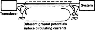
Figure 12.74 An earth loop formed by connecting both ends of a screened cable to the local earth. Screens should be earthed at one point only
High voltage and low voltage cables should be well separated, most manufacturers suggest at least one metre between 415 V and low voltage cables but this can be difficult to achieve in practice. In any case, separation can only be achieved until some other person, not knowing the system well, straps a 415 V cable to the same cable tray as a multicore thermocouple cable. It is therefore good practice to use trunking or conduit for low voltage signals as a way of identifying low voltage cables for future installers. The same result can also be achieved by using cables with different coloured PVC sleeves. Inevitably high voltage and low voltage cables will have to cross at some points. If spacing can not be achieved the crossings should always be at 90°.
In an ideal world, separate cubicles should be provided for 110 V/high current devices, and low voltage signals, but this is often not cost effective. Where both types of signals have to share a cubicle the cables should take separate, well separated routes, and high and low voltage devices separated as far as possible.