Power system operation and control are guided by the endeavour of the utility to supply electric energy to the customer in the most economic and secure way. This objective is underlined by the fact that the electric energy system is a coherent conductor-based system in which the load effects the generation without delay. Energy storage can only be realised in non-electrical form in dedicated power-stations, so that each unit of power consumed must be generated at the same time. It is therefore necessary to maintain all the variables and characteristics designating the quality of service, such as frequency, voltage level, waveform, etc.

The power system is operated continuously and extends geographically over wide areas, even over continents. The number of generators supplying the system and the number of components contributing to the objective are extremely high. However, the task of system operation is alleviated by the fact that there are not too many different types of component (if the intricacies of power-stations are excluded). In the transmission system the components that are quite easily managed are lines, cables, breakers, disconnectors, bus-bars, transformers and compensators. In the power-stations the generator commonly used is the synchronous machine. The prime mover is a turbine driven by steam or by water. Overlooking the details, there are similarities in the operation and control of turbines and generators that permit a certain uniformity of approach; however, many details have to be considered when it comes to design, failure modes, actual performance, quality of service, etc.

The mechanism of power flow in the system, which is a key issue in all considerations of operation under normal and disturbed conditions, is governed by the Ohm and Kirchhoff laws. Higher voltage at an appropriate phase angle will cause more power flow when a suitable path is available. To draw power from a system is extremely simple: the consumer’s load is just connected to a three-phase bus-bar, where the voltage is regulated so that the load can be supplied. The system includes control actions by which the power is allocated to various generators, but there is little interaction in the transmission system.

For economic and secure operation, the actions are quite sophisticated. Control can no longer be performed in a single location by observing a single variable. The control system becomes a multivariable, multi-level system with real-time and prophylactic interventions, either manual or automatic. Thus, the control system is a hierarchical system where the levels and corresponding functions can be characterised as follows.

Decentralised control:

(1) In the power-station: control of voltage, frequency, active and reactive power.

(2) In the substation: control of voltage (tap-changer on transformers), switching of lines and cables, protection.

Centralised control:

(1) Regional control centre: switching, start-up and shutdown of generating units, unit commitment, reactive power control and load frequency control.

(2) Utility control centre: economic load dispatching, security assessment, load frequency control (automatic generator control), power exchange with other areas, security monitoring, security analysis and operational enhancement.

A hierarchical control system needs extensive communication. Hence there is an extensive telemetering and telecontrol system which provides data to the various control levels and executes control actions at a particular location that have been initiated in a control centre.

The following material is organised in such a way that the objectives and requirements of system operating and control are given and discussed first (Section 40.2): they underline the motivation for the development of modern complex systems. A way of presenting components and subsystems is given in Section 40.3. Data acquisition and telemetering are then treated (Section 40.4) these are prerequisites for power system control.

Decentralised control is divided into excitation control (Section 40.5), turbine control (Section 40.6) and substation automation (Section 40.7), which are the most important control functions at a local level. Pulse controllers for tap-changers are also considered (Section 40.8).

Centralised control is dealt with in Section 40.9, where the hardware and software aspects of computer-based system operation are considered. With the various systems and functions to hand, present-day system operation is characterised in Section 40.10. Changes in the system operation due to liberalised energy markets are also pointed out in the Section 40.11. The new focus on distribution automation and demand side management is touched upon in Section 40.12. Finally, the reliability of system control is considered in Section 40.13.

40.2 Objectives and requirements

The often-cited objectives of economy and security have to be considered in various time-scales and in different system conditions in order to achieve a systematic approach to power systems operation, particularly when computer-based systems are involved. Before we go into details, it should be noted that system operation as considered here is a problem within the framework of a given power system. Planning problems and problems of procuring the primary energy are omitted.

Any objective or requirement is derived from the basic task of supplying electric energy to the consumer with the least expenditure of economic effort, measured over a long period. Hence a variety of cost items and even some intangibles such as environmental effects are involved. These items range from generating costs, losses, the cost of outages and the cost of damages, to risks and the amount of emissions, etc. Stated thus, these items are still too general to be converted immediately into an objective upon which a control function could be built. Different objectives apply for decentralised and centralised control; moverover, within a centralised control system it is necessary to distinguish various conditions to which particular objectives apply.

The most widely used concept for the realisation of a systematic control approach in centralised control is the concept of states. A state of the power system is characterised by reserves, by the ability of the system to override a disturbance, by the presence or absence of overloads, etc. The starting point is a series of considerations concerning the security of the system. However, considerations of economy can be easily added.

The four states with some rough characterisations are as follows:

(1) Normal (N) state: the system has no overloads and a good voltage profile; it can withstand a line or generator outage and is stable.

(2) Vulnerable (V) state: the system has no overloads and a good voltage profile; line or generator outage causes overloads and/or voltage droop; there is a low stability margin.

(3) Disturbed (D) state: the system still supplies its loads, but overloads are present and there is a low voltage profile.

(4) Emergency (E) state: the system cannot supply all of its loads, overloads are present, there is a low voltage profile and part of the system is disconnected.

There are inadvertent transitions between the states caused by faults, human error and dynamic effects. However, control actions will return the system to the normal state. A thorough understanding of system operation will show that appropriate objectives and corresponding control functions will effect this return in a logical manner. These mechanisms are illustrated in the schematic of Figure 40.1, which shows (upper part) a state diagram with various transitions. The lower part of the figure gives transitions associated with a number of objectives. These pertain to control actions only. It is clear that the objective of full load coverage has to be met first before the vulnerable state can be reached. Further, all vulnerable conditions have to be eliminated before economic dispatching can be initiated.

Figure 40.1 Security states and objectives: state diagram (above) and controlled transitions (below) following given objectives

At the decentralised level the objectives are much simpler and easier to understand. A state concept is not necessary since the objectives are expressed in terms of errors or time sequences in a straightforward manner. As an illustration, let us consider protection and excitation control.

In protection the objective is to keep fault duration or outage to a minimum. The fault itself cannot be avoided, but the adverse effects, possibly leading to a disturbed or emergency state, can be. Thus protection supports the aim of security on the decentralised level.

Excitation control maintains the voltage at a given location of the system and supports the stability. It is the stable voltage, with all its implications, that is at stake. A stable voltage is a very important prerequisite for system security. For its realisation many detailed considerations are required since it is system dynamics that determines the performance of excitation control. Beyond that, an excitation system has many monitoring functions, i.e. limit-checking and even protective functions. The objectives of decentralised control, which become recognisable in terms of set-points, time periods and the like, must be co-ordinated. This co-ordination is performed either in the planning or operational planning phase (e.g. for protective relays), or in real time (e.g. for economic dispatching).

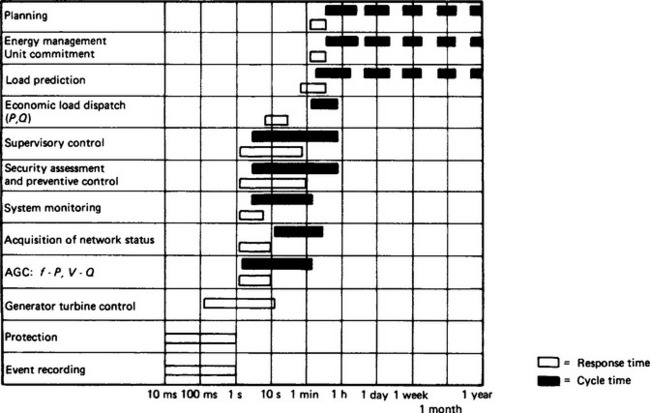
In power system operation and control it must be recognised that the control functions have a certain time range in which they are effective. Thus the corresponding objective has its validity within this time range only. As Figure 40.2 shows, there is a complete hierarchy of functions ordered in terms of their effective time range. This hierarchy in time is also responsible for the functional hierarchy of the control system.

Figure 40.2 Response times and cycle times for plant management, monitoring protection and control functions. AGC, Automatic generation control; P, active power; Q, reactive power; f, frequency; V, voltage

40.3 System description

In describing an electric power system we must distinguish the network (responsible for transmission and distribution) and the generating stations, as well as the loads.

The network is amenable to description by topological means such as graphs and incidence matrices as long as the connection of two nodes, by a line or cable, is of importance. Thereby it is implied that the connection is made by a three-phase line which is itself described by differential equations. This topological description is always inherent and necessary. In routine work, however, it may not always be obvious what the true background is. Hence it is worthwhile to consider these topological means as a starting point.

Graphs and incidence matrices are equivalent and describe the way in which nodes are connected. A graph is a pictorial representation, whereas the incidence matrix is a mathematical formulation which can be interpreted by a computer. An example will illustrate the correspondence between these two descriptions. Figure 40.3 shows a graph derived from an electrical network. The connections between nodes have been marked by arrows; this fixes the way of counting and thereby orientates the graph. Figure 40.4 is the incidence matrix corresponding to the graph. The way of counting is indicated by the sign of the entries. Both the graph and the matrix describe the same network. The graph, however, is much easier to grasp.

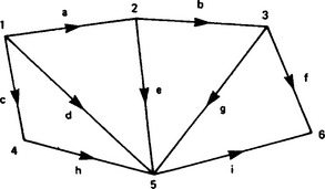
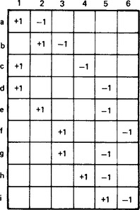
Figure 40.3 Oriented graph describing the structure of a six-node network: 1–6, nodes; a—i, lines

Figure 40.4 Nodal incidence matrix A corresponding to the graph in Figure 40.3. The matrix establishes relationships between line and nodal quantities (currents and voltages). The arrow leaving a node determines the positive sign of the entry (+1)

The incidence matrix is the base for two processes, both of which are important for systematic description. The first is the reading of network data, wherein the way in which lines are connected is already implied. The second is the establishment of admittance and impedance matrices.

Consider the graph in Figure 40.3 where the nodes have a particular numbering. This numbering permits the specification not only of a connection between two nodes but also of the type of connection. Assume that the connections consist of simple series impedances. Then the following description, which is machine-readable, is possible:

The first column specifies the nodal connection, the second the complex impedance. Each line of the list corresponds to a connection or a line of the network.

The generation of the nodal admittance matrix can be explained by a multiplication of the primitive admittance matrix _p(diagonal matrix) by the corresponding incidence matrix and its transpose from left and right respectively:

The nodal admittance matrix contains all the information necessary (topology, impedance) to describe the network.

Loads and generators are connected to the nodes of the network. The description of the nodal constraints depends on the way the network is employed in an analysis or decision-making process.

For the purposes of load-flow calculations the specification is done in terms of PQ- or PV-nodes, where PQ means that the active power P and reactive power Q at the node are constant (i.e. independent of voltage), and PV means constant active power and constant voltage.

For dynamic analysis more complex models for the nodal description have to be added. On the load side, the frequency dependence or, if necessary, a set of different equations is needed. For the generating unit, differential equations are comprehensive, but not always transparent. Hence, a block diagram is used to specify forward and feedback paths, wherever appropriate. As an example, the signal flow and the generation of torque within a turbogenerator are given by the block diagram in Figure 40.5. The dynamics of a synchronous machine would also be amenable to such a description, but in practice a description by differential equations (two-reaction theory) is usually preferred. Details of controllers and regulations are described by block diagrams, as is common in control engineering.

Figure 40.5 Schematic diagram of a generator and a speed governor: G, generator, T, turbine; R, regulator/speed governor; f, measured frequency; f_s, set-point of frequency

40.4 Data acquisition and telemetering

40.4.1 Introduction

To be able to supervise and control a power system, the network control engineer requires reliable and current information concerning the state of the network. This he obtains from the power flows, bus voltages, frequency, and load levels, plus the position of circuit-breakers and isolators; the source of these data being in the power stations and substations of the network. As these are spread over a wide geographical area, the information must be transmitted over long distances. Thus the electrical parameters and switch states must be converted into a suitable form for transmission to the control centre. A telecontrol system is also required to transmit these data using communication channels which were historically limited in capacity and were shared with other facilities such as speech, protection and, perhaps, also telex communication. Speed of data transmission was therefore often limited, and the telecontrol network was configured to optimise the use of the available bandwidth on the carrier channel. The modern communication is based on fibre optical or wireless communication networks, which provide a powerful broad band communication. The classical power line carrier communication technology has also been improved with the use of digital technology. It is almost mandatory that all the new HV and EHV lines be laid with fibre optical core in the ground wire, as the incremental cost is quite low. The trunk routes may have dedicated logical links for speech, data and protection signal in addition to the data and voice network for telecommunication purposes.

The telecontrol system comprises a master station communicating over communication channels with remote terminal units (RTUs) located in the power stations and switching stations. Normally the RTUs are quiescent, i.e. they only send data after a direct interrogation from the master station; thus more than one RTU can be connected to a transmission channel as the channel can be time shared. A telecontrol network can be configured as a point to point, star (radial) or multi-point (part line) system as illustrated in Figure 40.6. The transmission can be either duplex, half-duplex or simplex (in the case where data traffic is unidirectional). The newer generation of RTUs can remain quiescent and can report the data on their own initiative using a slave to master communication protocol. The use of standard telecontrol protocols is also being promoted to facilitate use of equipment from different suppliers. International Electrotechnical Commission (IEC) has recommended IEC870-5-xxx group of protocols, which allow certain amount of openness in the system. The state of the art RTUs can communicate over data communication networks providing a large bandwidth with good reliability.

Figure 40.6 Transmission network configuration

40.4.2 Substation equipment

The data-acquisition equipment in a substation is usually a microprocessor-based RTU, equipped with both programmable read-only memory (PROM) and random-access memory (RAM). The data-acquisition program and the transmission program are loaded into the PROM, which is non-volatile (not corrupted during a power supply failure). All the system modules are connected to the system bus (see Figure 40.7) which is structured to facilitate data transfer from the information source to its destination, under the control of the program. The microprocessor function is monitored by the watch-dog module. The RTU is configured to suit the substation requirements. A typical configuration is shown in Figure 40.8 with the input/output for one high-voltage (h.v.) circuit only. The input modules fall into three main categories: digital input, analogue input and pulse input.

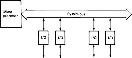
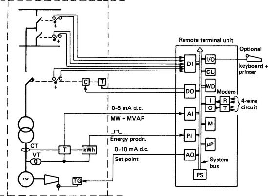
Figure 40.7 RTU bus structure: I/O, Input/output

Figure 40.8 Example of the configuration of a RTU: Dl, digital input; DO, digital output; Al, analogue input; PI, pulse input; AO, analogue output; μP, microprocessor; M, memory; CL, clock (optional); I/O, serial input/output interface; WD, watch-dog; PS, power supply; TG, turbine governor; CT, current transformer; VT, voltage transformer; T, transducer; CT, close, trip; R/T, receiver/transmitter

40.4.2.1 Digital inputs

Digital input modules are used for inputting contact states indicating breaker positions, isolator positions and alarm contact operation. The contact states are continually monitored but are not transmitted unless a contact state has been changed. Under program control, the module is cyclically interrogated to see whether it has a change of state to report: if the reply is negative, the program moves to another module; if it is positive, the change of state is written to the memory. The input circuits are decoupled from the power system equipment by electromagnetic relays or opto-couplers and are filtered to eliminate the effect of contact bounce. A digital input circuit is illustrated in Figure 40.9.

Figure 40.9 Digital input circuit

40.4.2.2 Analogue inputs

The electrical measurements are converted from current-transformer and voltage-transformer levels to analogous direct-current (d.c.) milliampere signals by suitable transducers. These convert voltage, current, active and reactive power, frequency, temperature, etc., into proportional d.c. signals which are fed into an analogue input module. This module (Figure 40.10) has a multiplexer for scanning multiple inputs (usually 16) and an analogue-to-digital converter (ADC) which converts the d.c. signal into a digital code (usually binary or BCD). The local scanning rate of the measurands is less than 0.5 s, with an accuracy of conversion for normal requirements of 1% for bipolar (7 binary bits+sign) values and of 0.5% for unipolar values. For higher accuracy requirements an accuracy of 0.1% is used (11 bits).

Figure 40.10 Analogue input module

40.4.2.3 Pulse inputs

Energy or fuel consumed can be measured by integrating meters giving a proportional pulse output. The pulses are integrated in a pulse input module which is periodically scanned, e.g. at 15 min intervals. The consumption over that period is then the difference between the last two readings. Special measures are taken to ensure that the reading does not interfere with the pulse integration or vice versa.

40.4.2.4 Digital output

Digital output modules convert a coded message, received from the control centre, into a contact output, e.g. to trip or close a circuit-breaker or to raise or lower a tap-changer. Obviously, the transmission of these signals must be very secure, and checking that the correct output is given must be rigorous. Echo checks are made to ensure that the correct code has been received by the module, and additional circuits can be added to detect stuck contacts and to prevent more than one command being output at a time.

40.4.2.5 Analogue output

Set-points are output via analogue output modules that receive a coded message which they convert into a d.c. analogue signal; this is output e.g. as a turbine-governor setting.

40.4.2.6 Clock

An optional feature of the RTU is a clock module, which enables the events in the substations to be arranged and transmitted in chronological order and the time at which an event happened to be added. The clock is capable of giving a 10 ms time resolution in event sequence recording and the time in hours, minutes, seconds and hundredths of a second.

40.4.2.7 Printer

A further option can be included to print the alarm and event sequences locally at the substation by adding memory, serial–parallel interface, a printer and additional program. If the memory capacity is limited, the output is either coded or abbreviated; however, with adequate memory the print-out can be in clear text.

40.4.3 Data transmission

The substation data are locally scanned and memorised in the RTU ready to be transmitted to the control centre. When an instruction is received from the master station, the processor prepares to send the data to the control centre. To every message containing data, it adds check bits that enable the master station to ensure that the message has not been corrupted during transmission. Similarly, to any message output from the master station, check bits are added to enable the RTU to verify that the received message has not been corrupted. The data are then output to the communication channel via the parallel-to-serial converter and the modulator-demodulator (modem) which converts d.c. pulses into keying frequencies in the voice-frequency (v.f.) range. Normally two v.f.-range frequencies are used to represent ‘1’ s and ‘0’ s of the message code and to modulate the carrier of the transmission channel. At the receiving end, the modem converts the keying frequencies into d.c. pulses and the serial—parallel converter module reassembles the message into a parallel word including the check bits. The message can then be checked for errors induced during transmission.

There are various methods of checking for errors in a message telegram. The error-detecting capability of a checking system is often described as a Hamming distance. The Hamming distance between two binary words is the number of bit positions by which they differ, which is undetectable by the error-checking system. For most purposes in telecontrol, the minimum Hamming distance is 4, i.e. all 3-bit errors are detected. An example of a modified Hamming code error-checking system is shown in Figure 40.11.

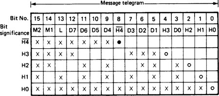
Figure 40.11 An example of message telegram organisation: •, odd parity check; ×, even parity check; x, bits supervised by Hamming bits; D, data bits; L, message sequence complete; M, message-type definition; H, Hamming bit

The advantage of this system is that in addition to detecting the same number of error patterns as equivalent error-checking systems of the same size, the introduction of odd parity in one check-bit position and even parity in the others forces at least two changes in bit settings in the telegram. This considerably reduces the risk of loss of synchronism when the word is being read. The Hamming distance of this code is 4: i.e. all patterns of 3-bit errors are detected, as well as all odd numbers of bit error patterns and over 92% of all even numbers of bit error patterns.

40.4.4 Transmission system

The data transmission system must be designed to allow all the RTUs to transmit their data to the control centre in a reasonable time without imposing impractical demands on the communication system. The data transmission can be divided into several parts, each of which can comprise one or more RTUs. Each part system is completely independent of the others; thus they effectively operate in parallel.

Three basic systems are possible: point-to-point, radial or multi-point (see Figure 40.6). Combinations of radial and multi-point are also possible.

With point-to-point systems, the transmission can be simplex (where the RTU sends data continuously to the master station) or half- or full-duplex (where data can be transmitted in both directions).

With radial or multi-point systems, the dialogue between the master station and the RTU is entirely controlled by the master station to avoid two or more RTUs sending data simultaneously. The master station transmits instructions to the RTU, which, in complying with the instruction, acknowledges it. The RTU takes no initiative in transmitting data and sends data only after receiving a specific instruction to do so from the master station. Thus all data in a part system are transmitted from each RTU in turn and response times are a limiting feature of a part system configuration.

There are two basic forms of data to transmit: even-controlled data which appear at random intervals, and data that must be transmitted cyclically as they are liable to be continually changing. The cyclically transmitted data, e.g. measurands which require frequent updating at the control centre, take up most of the transmission time; however, as the RTU is quiescent, periodically it must be asked whether it has any spontaneous data to transmit. To save transmission time, this is made in a ‘broadcast’ interrogation to all RTUs in the part system simultaneously. If no RTU answers positively, the normal cycle sequence is resumed; however, if one or more RTU answers that it has spontaneous data to send, the normal cycle is interrupted and each RTU is interrogated in turn until all the spontaneous data have been transmitted and received at the master station. In order that the detection of spontaneous data (e.g. a breaker trip) is transmitted in a reasonable time, the spontaneous data interrogation is interjected between the transmission of groups of measurands (say 16). An example of a transmission sequence is given in Figure 40.12. The spontaneous data can be sent in chronological order of events taking place and also with the time at which each event happened.

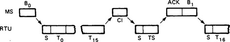
Figure 40.12 A typical transmission sequence: B_n, call for transmission of a group of measurands; S, start character; T_n, values; CI, call for transmission of a change of state; T_s, change-of-state message; ACK, acknowledgement of receipt of meassage; MS, master station

The response times are dependent on the transmission speeds, and a choice of speed is available. Standard speeds of 50, 100, 200, 600 and 1200 bit/s are available within the v.f. band. The choice of speed is then dependent on the response times required and the bandwidth available on the communication channel. As an example of response times, a part system comprising four RTUs each having measurands would have a measurand and indication interrogation scan time (with no changes of state to transmit) of approximately 6.5 s, using a 200-baud channel. To decrease this time, either the number of RTUs in the part system would have to be reduced or the speed of transmission would have to be increased.

40.4.5 Communication channels

The transmission of the frequency-shift keying signals requires a four-wire circuit communication channel, which can be telephone-type cable, power line carrier equipment, radio transmission or any combination of these media in series or parallel. Figure 40.13 gives an example of a possible combination of different types of communication channels.

Figure 40.13 An example of a data transmission system. Tx, Rx, radio transmitter and receiver; PLC, programmable logic controller

Often the telecontrol signal must share the v.f. band with other transmissions such as speech, telex, protection or even another telecontrol part-system transmission. An example of the frequency multiplexing of the v.f. band is given in Figure 40.14. The multiplexing equipment is normally available with the power line carrier. The frequency-shift keying takes place within the frequency bandwidth indicated in Figure 40.14: e.g. for a 200-baud modem the lower keying frequency is −90 Hz and the upper is +90 Hz of the channel centre frequency. The total bandwidth required is 360 Hz.

Figure 40.14 Allocation of communication functions to a 4 Hz channel

40.5 Decentralised control: excitation systems and control characteristics of synchronous machines

40.5.1 Introduction

A synchronous generator operating on an interconnected grid requires a fast-response excitation system to ensure its stable operation. This system must be able to adjust the level of magnetic flux in the generator according to the grid network requirements. Since the parameters of the generator will fall into a fairly narrow range according to the type of generator (salient pole or turbo), the excitation system must be designed to bring the generator flux (i.e. excitation current) to the required level in the shortest possible time, notwithstanding the long time-constants of the generator transfer functions.

Brushless excitation equipment has been developed to meet these requirements on various types of synchronous generator—particularly on smaller turbogenerators—and has given excellent results in service. The control characteristics of this system, however, are dictated largely by the exciter and the rotating diodes rather than by the voltage regulator (d.c. exciters are not used in modern excitation systems).

For large generators a static excitation system represents the best solution since, in principle, it imposes no limit on the ceiling voltage. In the per-unit system the ceiling voltage is the ratio of the maximum excitation voltage to the excitation voltage for nominal open-circuit voltage at the generator terminals. Values of 10 or 15 p.u. are quite often used. A great advantage of static excitation is that the total field-voltage range is available with practically no time delay. This speeds up not only field forcing but also field suppressions when required, by change-over to inverter mode.

40.5.2 Brushless excitation systems

Brushless excitation systems are mainly employed either where the control requirements are not too stringent or where the atmosphere is chemically aggressive. The main generator excitation is provided by an auxiliary exciter generator mounted on the main generator shaft.

This exciter is a salient-pole synchronous generator with a three-phase winding on the rotor and a d.c. excitation winding on the stator. The alternating currents produced by the rotor winding are rectified by rotating diode bridges mounted on the shaft, the resulting d.c. being fed to the field winding of the main generator. The excitation for the exciter stator winding is supplied by a thyristor regulator which comprises voltage regulators and limit-value controllers. Field suppression of the exciter machine is also carried out by the regulator (Figure 40.15):

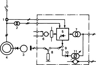
Figure 40.15 Voltage regulation system with manual control facility: 1, current transformer; 2, voltage transformer; 3, exciter; 4, generator; 5, voltage regulation; 6, reference value; 7, supply transformer for the voltage regulator; 8, field switch/discharge resistor; 9, change-over switch; 10, rectifier; 11, variac with motor drive

The controlled rectifiers and the electronic circuitry of the regulator are supplied either from a permanent magnet (p.m.) generator on the main shaft or through a transformer fed from the main generator terminals. In the latter case, compounding equipment is available for the required selective switching (short-circuit duration in excess of 0.5 s) which is then combined with the standard regulators.

In its basic form the regulation system contains the continuously active elements for automatically controlled operation, which are;

(1) a voltage regulator;

(2) a reference-value potentiometer for remote adjustment;

(3) a supply transformer;

(4) a field-breaker and discharge resistors; and

(5) diode monitoring consisting of the manual control device, i.e.

(a) a variac transformer,

(b) a diode bridge, and

40.5.3 Static excitation systems

On generators with difficult regulation requirements a rotating exciter should not be used. Here the excitation is supplied either directly from the generator terminals via a transformer and a controlled rectifier bridge (Figure 40.16) or by an auxiliary generator.

Figure 40.16 Block diagram of a voltage regulator with static excitation (without manual control): 1, instrument transformer; 2a, transducer; 2b, voltage regulator; 2c, PID filters; 3a, firing-angle control; 3b, filter; 3c, voltage relay for control of excitation field flashing; 4, pulse amplifier; 5, reference-value setting unit; 7, generator; 8, main excitation rectifier; 9, excitation transformer; 10, field suppression device; 11, field flashing device; 12, overvoltage protection

The main components of a static excitation system are:

(1) an excitation transformer (or auxiliary generator);

(2) a static converter;

(3) a field suppression system;

(4) control and firing circuits; and

(5) a protection and monitoring system.

The capacity of the excitation system is dependent on the generator specification and on the requirements of the power system. The rating of the excitation transformer or exciter in particular is determined by the maximum continuous current rating of the rotor winding and the required ceiling voltage. In designing the converter circuits, which have much shorter thermal time-constants, the ceiling current and short-circuit current capacity must also be considered.

The voltage of the transformer secondary (or of the auxiliary generator) is determined by the maximum ceiling voltage, V_c of the excitation system, and its current by the maximum continuous current I_fm of the generator field winding. A simple approximation to the rating of a three-phase excitation transformer is 1.35 V_cI_fm.

The static converter comprises one or more fully controlled thyristor bridges, which are almost always cooled by forced air. The number of parallel bridges and the number of series elements in each bridge branch are determined by the technical data (current rating and inverse voltage) of the thyristor bridges, the maximum exciting current, the transient overload (due, for example, to a system fault) and the ceiling voltage. An extra redundant bridge is normally included (in parallel) so that, even if one bridge fails, the full operational requirements can still be met. To ensure selectivity, it is necessary to have at least three bridges in parallel. This is because a faulty thyristor together with a healthy branch can form a two-pole short circuit that persists until the fuse in series with the defective element blows. If only two parallel bridges are provided then the short-circuit current in the healthy branch is shared by only two thyristors; the fusing integral of both the corresponding fuses may then be exceeded, resulting in an excitation trip.

The rectifier can have either a block structure or be arranged phase by phase. In the block arrangement, one or more bridges are grouped together and gated from a common pulse amplifier. Blocks are normally provided with individual fans, but common cooling is also possible.

The arrangement of the converter in phase groups reduces the risk of an interphase short circuit. All parallel thyristors of one phase are brought together in a single rack. A separate cooling system for each rack is inappropriate in this arrangement and common cooling is employed, consisting of two fans each capable of supplying the full cooling-air requirement.

With the phase-by-phase arrangement, the excitation transformer is usually composed of three one-phase units; this will always provide a higher degree of safety against interphase short circuits.

The field suppression system comprises essentially a two-pole field-breaker and a non-linear field discharge resistor. The component ratings are so chosen that neither the permissible arcing voltage at the breaker nor the maximum permissible field-circuit voltage is exceeded, even with the maximum possible field current (following a terminal short circuit on the generator). A ‘crowbar’ is included in the discharge-equipment cubicle as additional overvoltage protection. This comprises two antiparallel thyristor groups which are triggered by suitable semiconductor elements such as breakover diodes (BODs). If, for instance, a voltage is induced in the rotor field circuit owing to generator slip, this voltage can rise only to the threshold of the BOD element. If this value is reached, the element triggers the thyristors, and the rotor circuit is connected to the discharge resistance, allowing a current to flow which immediately causes the induced voltage to break down.

40.5.4 Automatic voltage regulator and firing circuits for excitation systems

The voltage regulator for brushless exciters as well as for static excitation systems constitutes the central control element in a modern plant. This unit uses a voltage transformer to measure the actual value, rectifies it and compares it with the reference value. The difference-voltage is fed to an amplifier with a lead—lag filter (the response characteristics of which must be carefully adjusted to suit the particular generator and grid parameters) and the amplified value is brought to the gate control unit. Using additional reactive current compensation it is possible to adjust the reactive current behaviour of the generator with regard to the network.

The voltage regulator has normally to be supplemented with parallel-connected limiters which function before corresponding generator protection relays are activated. Depending on requirements, rotor-current, load-angle and stator-current limiters may be employed. Their features are described later.

If the limitation control causes a reduction in the excitation current (on over-excited operation), time-delay elements are incorporated to allow high transient currents. For underexcited operation there is no time delay.

Stabilising equipment can be used to damp power oscillations that may arise under exceptional network conditions.

The voltage regulator may be supplemented with an overriding system for controlling the power factor or the reactive power flow, as required. All voltage regulators are provided with manual control (changeover from closed-loop to open-loop control). A separate redundant gate control unit is often provided (double-channel type). In case of a fault in the ‘automatic’ channel, a follow-up control system ensures a smooth transition to manual operation.

The amplified difference signal is transformed into pulses with the appropriate firing angle by the gate control unit. The firing pulses are amplified in an intermediate stage and led to the individual output stages which are assigned to the various converter units. The output stages shape the pulses to the steep slopes necessary to ensure simultaneous firing of all parallel thyristors. The pulses from the output stages are fed via impulse transformers to the thyristor gates.

The transfer function of the automatic voltage regulator (AVR) including the gate control system is

where T_M is the measuring time-constant, T_E is the exciter time-constant, T₁, … T₄ are the equivalent lead-lag time-constants, A is the amplification, and p is the operator d/dt.

40.5.5 Limiting the excitation of synchronous machines

Ever-increasing demands on power system reliability led to the development of ancillary equipment (limiters), to inhibit the tripping of protection gear when this was not wanted and to make, within the permissible limits, better use of the synchronous machine. These limits are clearly depicted in the power chart of a turbogenerator shown in Figure 40.17.

Figure 40.17 Current and power diagram of a turbogenerator (I = 1 p.u.; V = V_k = 1 p.u.; X_d = X_q = 2 p.u.; cos ψ = 0.8): I, underexcitation; II, overexcitation. AB, Practical stability limit; AB′, steady-state stability limit; BC, limit of stator temperature rise; CD, limit of rotor temperature rise; CE, active power limit; E rotor e.m.f.; I_b, reactive current; I_e, excitation current; I w, active current; P active power; Q reactive power; V_k, terminal voltage; X_d, direct-axis reactance; X_q, quadrature-axis reactance; δ, load angle; ϕ_n, rated phase angle

The limit of active power output (line CE) is determined by the prime-mover, and is disregarded. A factor connected directly with excitation current, however, is the permissible temperature rise in the rotor winding, represented by the arc CD with centre A corresponding to the non-excited condition. This thermal limit is defined by the ageing of the insulation. It may therefore be exceeded for a short time—a requirement essential for the stability of the power system.

In the underexcited mode, operation of the synchronous machine is limited by the airgap torque necessary for the active power transfer, the steady-state condition being represented by a definite, permissible rotor displacement angle (line AE). This limit has mechanical and dynamic characteristics, and calls for instantaneous intervention as soon as it is exceeded, to prevent the generator from falling out of step.

Another important condition governing the limits to be introduced is the requirement that these do not interfere with the normal operation of the voltage regulator, and that neither intervention nor return to voltage regulation leads to disturbances.

Electronic load-angle and current-limit controllers were introduced some time ago, and these are now standard components of all good voltage regulation equipments. Practical experience has made possible the addition of improvements and refinements.

Consider the static excitation equipment commonly used for large generators (Figure 40.18). Normally, the voltage regulator holds the generator voltage (and thus, indirectly, the reactive power output) at a constant level. The static converter adjusts the excitation current so that the reference voltage remains a function of the reactive current. At the same time, the rotor-current limit controller measures the excitation current in the static converter supply and compares it with the relevant reference limit. The load-angle limit controller continuously forms from the generator current and voltage a signal that is proportional to the angle, and compares it with the limit.

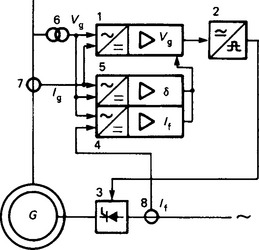
Figure 40.18 Block diagram of the automatic voltage regulation system for a synchronous generator: 1, voltage regulator; 2, gate control unit; 3, static converter; 4, rotor-current limiter; 5, load-angle limiter; 6, voltage transformer; 7, generator-current transformer; 8, excitation-current transformer; G, synchronous generator, V_g, generator voltage; I_g, generator current; I_f, rotor current; δ, rotor angle

The two limiters operate as parallel controllers, i.e. their signals completely replace the voltage as controlled variable when their output variables become smaller or greater than the voltage control signal. Thus, the change in specific dynamic behaviour of the control circuit for each limit function can be fully taken into account. It will be shown that unwanted side-effects occurring on signal take-over can be avoided entirely.

40.5.5.1 Rotor-current limitation

Every exciter is capable of delivering a maximum current appreciably greater than the continuous value based on thermal considerations. This capacity for overexcitation is necessary to provide the additional reactive power demanded during selective clearance of faults and to maintain a synchronous torque even when the voltage level has fallen.

Although it safeguards the winding insulation against damage from prolonged overexcitation, rotor protection gear (such as overcurrent and overtemperature relays) disconnects the generator even when disconnection is not desired. Use of a controller to limit the excitation current to an acceptable value during operation would substantially improve the availability of the generator. For safety reasons, however, a separate protective device must be retained to safeguard the winding against overloading.

The demands to be met by the rotor-current limiter are best explained with reference to the voltage and excitation current when a short-line fault occurs. The voltage regulator reacts to the drop in voltage with surge excitation. The controller is not intended to impede this, but merely to determine the ceiling current I_fm. Although the clearance normally takes place in a few hundred milliseconds, the longest duration (back-up protection) of 2–3 s will be assumed. When, after the fault has been cleared, nominal voltage is attained with a permissible continuous excitation current, the thermal controller will not intervene. However, when because of, for example, breaker failure the fault is not cleared, or when generated reactive power no longer suffices to maintain the voltage level, overexcitation will continue to be present. The limit controller now aims to reduce the excitation current before any of the protection gear is tripped. A further important aspect is that this also causes the short-circuit power of the system to be reduced, which, in turn, will diminish the extent of the damage resulting from failure of a breaker or other protective gear.

The condition in which the maximum continuous excitation permissible is present might persist for a long time, and experience has shown that further short circuits appear relatively frequently during this time. When these secondary disturbances occur, it becomes necessary to deliver the maximum reactive current to the system once more, especially to retain system stability. This means that limitation has to be cancelled again for a short time. The characteristic which trips the reset is the steep drop in voltage, dV/dt.

A further requirement results form the fact that today most of the large excitation equipment is fed from the generator terminals. The necessary ceiling excitation current is normally already available at 90% of the rated voltage. This means that at 120% of the rated voltage, a ceiling current which is 33% higher than the necessary value will flow when an instantaneously acting excitation limiter is not provided.

The limitation signal can be introduced as a reference-value variation of the voltage regulator. However, two facts suggest applying the signal to the voltage regulation output for use as dominant parallel limitation. These are: (i) the limitation is absolute and thus fully effective even when the actual value for the voltage regulator is lost (voltage-transformer fuses blown); and (ii) the limit controller can be adapted to the dynamic conditions of the field-current controller and become independent of voltage-regulator response.

As has been mentioned, limitation to the permissible continuous excitation current should be delayed in order to first give the voltage the maximum support possible. The permissible continuous current in the excitation circuit is determined by the thermal stressing of the field winding, the supply transformer, or the thyristors or diodes. The overload capacity of these elements can usually be represented by integration of the current. A slight overrun of the set limit for the continuous current is then tolerated correspondingly longer. It can be argued, however, that the ceiling excitation will be required only as long as fault clearance is still taking place, in which case a fixed timing element is provided. In both cases, it is usually desired that ceiling excitation should be available again in the event of secondary disturbance.

Based on previous experience, improved rotor-current limit controllers were developed to cater for the many varied applications met with in practice; these controllers can be easily adapted to the particular protection method used.

A maximum-current limit controller, instantaneous acting and always available, ensures that for terminal-fed excitation the desired ceiling current is not exceeded over the entire operating voltage range.

In the case of the simple integrator mode, the speed at which reduction to the limit value takes place is relative to the magnitude of the overcurrent. The integrator is reset only when the limit for the continuous rotor current is underrun.

With the switching mode, reduction to the limit begins after a set delay T_v of several seconds. Every time there is a sharp drop in voltage, maximum-current limitation begins anew and the timing element is reset.

A method frequently used in the combined mode: here, integration of the overcurrent is combined with resetting of the integrator by each succeeding voltage drop.

The actual current can usually be measured with a current transformer in the alternating-current (a.c.) power supply prior to rectification by the thyristors or diodes. A d.c./d.c. converter makes connection to a shunt also possible.

When partial failure of components in the excitation circuit causes the permissible continuous current to be reduced, change-over to a pre-set second current limit set-point is possible.

40.5.5.2 Load-angle limitation

For a number of years it has been standard practice to provide protection gear that detects excitation failure or loss of generator synchronism and trips the generator breaker. Inadequate excitation can, for example, also be caused by a change in the system configuration due to a fault, by reference-value failure or by other faults in the voltage regulator. The load-angle limiter obviates unnecessary disconnection by the under-excitation protection device in all these cases.

The limit angle is set intentionally to a value considerably smaller than the pull-out limit. For turbogenerators, for example, the angle lies between 70° and 85°. For salient-pole machines the actual stability must be taken into account and a suitable response limit determined. Thus, an adequate angle difference exists for the acceleration of the generator during clearance of a nearby short circuit. This reserve is directly related to the time allowed for clearing the fault.

The principle of analogue simulation of the phasor diagram using stator voltage and current is applied. This method is notably simpler than the direct measuring processes. In the event of a transmitter on the shaft providing the rotor position, the same device may be employed for further evaluation. The angle between the two simulated phasors, rotor voltage E_p and the infinite bus voltage V_s, is converted into a d.c. signal in a solid-state angle discriminator. When transients appear, the angle generated by the simulation leads the true load angle slightly. This is advantageous as this limiter should intervene at an early stage. Such a procedure has been shown to be reliable in practice.

40.5.5.3 Stator-current limitation

The stator-current limit, which is governed by thermal considerations, normally lies beyond the operating range of the synchronous generator. Thus, stator-current limitation is employed only in special cases. To illustrate this point, actual applications of a stator-current limit controller, usually in conjunction with limit control of the load angle and excitation current, are given below.

(1) With gas turbo-sets, for example, the useful output can be raised at times to cover peak demands, so that the limit is governed partly by the stator current.

(2) In coastal areas it is necessary to reduce the system voltage at certain times of the year because of salt vapour; there is thus an increase in stator current for the same power.

(3) In the case of reactive power compensators the under-excitation limit can be attained only with a stator-current limiter.

(4) With synchronous motors, a practical utilisation limit can appear that will be detected approximately by a stator-current limit controller.

40.5.6 Control characteristics for synchronous machines

As far as the system of synchronous generator and network is concerned, there is a strong similarity between the speed and active-power control system on the one hand, and the voltage and reactive-power control system on the other. To understand control by characteristic it is useful to compare the two systems (Figure 40.19). As long as the set is operating at no load, or on isolated duty, the appropriate value is controlled by the corresponding control system, i.e. the speed (frequency) or generator voltage. This is no longer the case, however, in parallel operation with a live network. Frequency and voltage are already present and can be changed by the set only to a limited extent. Secondary controlled variables are involved here, and it is imperative that they are controlled in parallel operation. These secondary variables are the active and the reactive power.

Figure 40.19 Characteristics for parallel operation: (a) speed/active-power control; (b) voltage/reactive-power control. 1, Generator breaker; 2, generator; 3a, speed regulator; 3b, voltage regulator; 4, turbine; 5, rotor winding; 6, network; P, active power; Q, reactive power; n, frequency; V, voltage

On what is this two-fold nature of the control system based? In isolated duty, only one control system is acting on any control loop. In parallel operation, however, many loops are coupled through the common controlled variable. The primary control task is distributed over a large number of control points. Selective stable distribution is of decisive importance. The overall task here is to maintain frequency and to produce active load, or to maintain voltage and to produce reactive load. The familiar solution is to provide the regulator with a drooping characteristic, i.e. the set-point of the primary controlled variable drops as the secondary controlled variable rises. The point of intersection of this characteristic of the network rating defines the corresponding operating conditions. Any set-point can also be set for the secondary controlled variable by parallel displacement of the characteristic. The gradient of the characteristic is usually expressed as a droop of the form S_n = Δn/n or S_v = ΔV/V, i.e. as the percentage deviation in the primary controlled variable that is necessary to bring the secondary controlled variable from zero to the rated value.

While the frequency of the network is the same throughout, in the case of voltage this applies only to the imaginary voltage of an infinite bus-bar. The true network represents roughly a variable ‘mountain landscape’ of voltages defined by its line impedances and feed-in or feed-out at a large number of junction points. This true network must first be accessible by reducing it to a simple equivalent circuit (Figure 40.20).

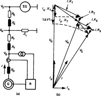
Figure 40.20 Impedances and voltage drops: (a) equivalent circuit diagram; (b) phasor diagram. V_s, Voltage of infinite system; V_N, system voltage; V_G, generator voltage; I, generator current; I_P, active component; I_q, reactive component; X, external (short-circuit) reactance; X_T, transformer reactance; X_D, direct-axis reactance of generator; E_E, R_T, active resistances; Z_L, load impedance; G generator; ΣG, sum of all other generators; R, voltage regulator

Each individual generator feeds through transformer and line impedances into the ‘finite bus-bar’ formed by the sum of all the other generators. As can be seen from the phasor diagram in Figure 40.20, which may be considered as qualitative, the products of the reactances and reactive components of the current are decisive for the magnitude of the voltage drop |ΔV|. The drop in active voltage and the phase displacement of the voltage phasor can here be ignored. The reactances between the generator terminals and the infinite network thus produce a natural drop in the reactive current, whereas the drop of the speed-control system is always synthetic. The generator reactance X_D is within the control loop and therefore need not be taken into account for quasi-steady-state phenomena. The effect of the natural drop in reactive current, and its increase or decrease by artificial means, is the main theme to be discussed from various viewpoints in the following.

40.5.6.1 Parallel operation in a power-station

Parallel operation in a power-station is illustrated in Figure 40.21. As virtually all large generators are operated in unit connection, the transformer reactance between the terminals and the h.v. bus-bar causes a natural reactive current droop of 8–12%. This accurately defines the reactive power output. Conditions are very different in the case of low-voltage (l.v.) generators, which must operate in parallel direct at the machine terminals. Here there is no natural droop, and even the smallest difference in the voltage values will lead to undesirable mutual exchange of reactive power between the machines, without resulting in a defined distribution of demand. It is not until an artificial droop is introduced by applying reactive current in the measuring loop of the voltage regulator that the reactive load distribution becomes stable; initially it is immaterial whether the generators themselves define the voltage at a purely consumer network, or coincide with the voltage given by a live network.

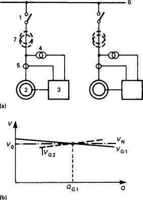
Figure 40.21 Parallel operation in a power-station: (a) basic circuit diagram; (b) characteristics. 1, Generator breaker; 2, generator; 3, voltage regulator; 4, voltage transformer; 5, current transformer; 6, bus-bar; 7, unit-connected transformer; V_N, system voltage; V_G1, V_G2, generator voltage characteristics; V₀, no-load voltage; Q_G1, reactive power output of generator 1

Electronic controllers have no dead-band and permit closed-loop gains of between 100 and 200 in accordance with a proportional range of 1–0.5%. Consequently, in isolated duty a satisfactory distribution over the parallel generators is achieved even with a 3–4% artificial droop. For reasons discussed later, there are various factors that make higher droop values more suitable for interconnected systems. The polygon connection used previously in some power-stations for distributing the reactive load has therefore lost its significance to a large extent because total elimination of changes in the steady-state voltage had to be bought at the cost of complicated circuitry.

40.5.6.2 Principle of current bias

The principle of phasor addition of a current-proportional voltage to the generator voltage has been known in various forms for some time (Figure 40.22). All three-phase voltages should be measured in each case to keep ripple and filter time-constants small. As shown in Figure 40.22, a one-phase current bias can be applied. In the case of controllers for large generators, the extra cost for symmetrical three-phase bias is justified.

Figure 40.22 Current bias: (a) basic circuit diagram; (b) phasor diagram; (c) characteristics. 1, Three-phase voltage transformer; 2, current transformer; 3, load resistance R_B; 4, rectifier; 5, voltage regulator; 6, generator; V_c, V, r.m.s. voltage; I_Rp, active current in phase R; I_Rq, reactive current in phase R, I_q, reactive current, superexcited; I, reactive current droop; II, no effect; III, reactive current compounding

The summation is made such that the overexcited reactive component of the current increases the actual voltage. This method of falsifying the actual value in relation to an unchanged set-point results in a drooping characteristic. In a steady-state condition the effect is the same as that of a reactance. A subtractive current bias causes a rising characteristic, i.e. a compounding. The effect of a true reactance can be reduced by compounding. In simple circuits the reactive current droop is accompanied by a slight compounding in the active current, but in most cases this is useful and under no circumstances is it a disturbing influence.

It should also be noted that the current bias curve is not entirely linear but slightly progressive. This is of virtually no significance. The current bias can be varied between zero and maximum by altering the load resistance. Nearly all voltage regulators are issued with this equipment.

As mentioned above, the current phasor is chosen in most cases so that an almost purely reactive load effect is created.

However, an active-load effect or a mixture of the two effects can be achieved by selecting a different phase angle. Consequently, in medium-voltage networks, additional active current compounding has shown itself to be a suitable means of improving the operating behaviour.

40.5.7 Slip stabilisation

Power transmission between synchronous machines and the load centre must remain stable even over long distances and under complex conditions. Experience has shown that certain network conditions can cause excessive hunting. Analysis indicates that hunting can be effectively reduced only by the introduction into the voltage control circuit of transient stabilising signals derived from the machine speed/frequency or produced by a change in the electrical output of the generator. Knowledge of the origin of the instability and the means of intervening in the controlled synchronous machine are essential for applying additional signals.

If the synchronous machine is connected to a rigid network through a reactance, it can be easily seen from the phasor diagram that the terminal voltage of the machine and the electrical torque alter with the rotor angle and with the main flux. The changes in terminal voltage, torque and main flux are given by differential quotients. In order to be able to make a quantitative statement for a given duty point, small changes are observed and the transmission functions and their representative factors are linearised about the duty point (index 0). This gives simple expressions, and a block circuit diagram (Figure 40.23) can be drawn which characterises the response of the synchronous machine at the rigid network. Let

Figure 40.23 Block circuit diagram of a synchronous machine connected to a rigid network: D, damping constant of synchronous machine; k, k_E proportionality factors; M_dE, electric torque; M_dM; mechanical torque; T′_d0, T_E, time-constants; T_m, moment of inertia; ω_m, angular velocity of synchronous machine; p, operator d/dt; other symbols, as for Figure 40.17. For linearisation of transfer functions assuming small changes:

The relationship between change in torque and change in rotor angle in a closed voltage-regulator loop is therefore

The factors, k₁, …, k₆ have a considerable influence on the damping of the synchronous machine and its behaviour, as follows.

k₁ is generally positive and can assume negative values only at correspondingly large network reactances, but it is then no longer possible to transmit stable power. In the normal range, however, this factor has a stabilising effect, i.e. damping.

k₂ is always positive and has a stabilising effect.

k₃ is independent of the rotor angle and responds only to changes in excitation.

k₄ is negative and reduces damping in the system, an effect that can be markedly reduced by high gain in the voltage regulator. The negative electric torque generated by k₄ is synchronous with the torque achieved with k₁ and is compensated by this.

k₅ comprises two components. With large system reactances x_e, i.e. where the rotor angle is large anyway, the expression can become negative. A torque that reduces damping is generated and is further enlarged by the gain at the voltage regulators. Active-load hunting commences with large amplitudes and leads to the machine losing synchronism and being shut down. Only with slip-stabilisation equipment can the effects of this component be eliminated and stable power transmission restored.

k₆ is independent of rotor angle and therefore of no significance as far as hunting is concerned.

It can be seen from the block circuit diagram that the damping-reducing influence is introduced through the difference between set-point and actual values at the voltage regulator. Provided that the synchronous machine is not equipped with static excitation, it is recommended to feed the stabilising signal to the mixing point of the control amplifier. Where static excitation equipment is provided, mixing is also possible direct at the entrance of the gate control system of the power stage of the excitation equipment. To damp the rotor oscillations, it is essential that more active power is delivered at the stator terminals when the rotor is accelerated, and less when it is braked.

There are various means of measuring speed and acceleration, and their corresponding effect on the rotor motion. One simple method is to measure the active power. Assuming that the prime-mover power is constant, changes in the active power cause corresponding acceleration or deceleration of the rotor. Measuring the active power fluctuations gives the first derivative of speed. The actual speed can be determined by integration. The accuracy of the method is adequate for this purpose. However, the reaction to load changes at the drive end is entirely false. Any danger to operation can safely be eliminated by limiting the effect of the stabilising equipment on the voltage control and by introducing an additional signal that is also proportional to frequency.

Thus the use of Δf, i.e. the angular frequency (Δω), instead of integration of ΔP represents a considerable advance in this field. The base signal combination (Δω plus ΔP) arrangement therefore gives the best arrangement for damping of oscillations (Figure 40.24). Test results have fulfilled all expectations in respect of the stabilising signal. Peaks in the signal, which occur when breaker operations take place in the network, are of such short duration that they have no effect upon the excitation. The load/frequency system combines the advantages of load and frequency measurement without any detrimental side-effects.

Figure 40.24 Δω+ΔP base signal combination arrangement for damping of oscillations, MU

40.5.8 Adapted regulator for the excitation of large generators

The excitation of a generator is in principle controlled by automatic voltage regulators, and improvements have been achieved in several respects. The original purpose of the feedback arrangement was voltage regulation. This basic requirement is important for maintaining stable synchronous operation of the generators in the power system and for controlling the voltage supplied to customers. Further advantages have been obtained since static (power semiconductor) excitation systems have been used. Through these fast-acting devices, the regulator may contribute to the transient stability after faults (keeping the generator from falling out of step) and to the damping of electromechanical rotor oscillations. Furthermore, stabilising signals have been introduced with pre-set amplification gains as a compromise to various operational points. These features are now provided by many commercial regulators. The adapted regulator improves the performance one step further. The main result is the good damping provided for a wide region of operating points, and the smooth voltage regulation.

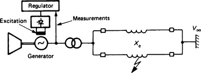
For better understanding of the benefits of an adaptive control on a network, the one-machine system is presented in Figure 40.25. The generator is connected to the ‘infinite bus’ V_∞ over two transmission lines with circuit-breakers. V_∞ is an ideal three-phase voltage source, and the lines are represented by pure reactances. X_e denotes the equivalent reactance between the generator and V_∞. This configuration corresponds to the realistic case of a remote power-station supplying a distant load centre.

Figure 40.25 Power system model

The control quality of the synchronous machine is assessed in terms of the steady-state behaviour and the dynamic performance in the presence of disturbances. Two kinds of disturbance must be considered.

(1) short circuits in the network, line switchings;

(2) changes of operating point (power, voltage, network parameters).

Therefore in the design of the voltage regulator the following performance criteria must be considered.

(1) Regulation of the generator terminal voltage with regard to: (i) smoothness (no ripple during steady-state operation); (ii) speed of response (to avoid overvoltages after load or topology changes); and (iii) accuracy.

(2) Ability to keep synchronism after a fault. This requirement means simply that the excitation voltage should be at the maximum during faults and during dangerous rotor accelerations. The excitation may return to normal after the first peak of the rotor swing.

(3) Damping of rotor oscillations.

(4) Criteria (1)–(3) for a wide region of operating points of the generator (power loading, voltage).

The voltage regulator used here corresponds to the present-day conventional regulator as described earlier. However, the stabilising signals derived from power and frequency measurements are introduced via variable gain factors (Figure 40.26). P and ω feedback are regarded as additional signals, the purpose of which is to produce damping (stabilisation) of rotor oscillations.

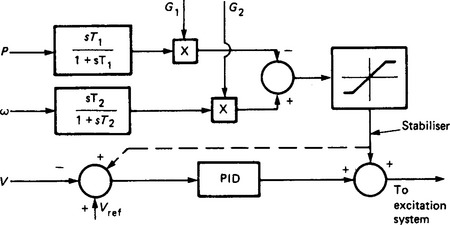
Figure 40.26 The analogure regulator (present-day Brown Boveri Cie (BBC) regulator). …, Alternative connection required by some customers

The gains for the power and frequency feedback are determined by using the D-decomposition technique. D decomposition (or domain separation) is a method based on the characteristic equation of the linearised model. It produces curves of constant damping in the plane of the gains G₁ and G₂, at a certain operating point (P = constant, Q = constant) and constant line impedance X_c. The method is combined with an optimisation procedure to generate optimal gains (optimal damping of the dominant poles). However, as already stated, the gains that are adequate for the best damping of rotor oscillations depend on the operating point of the generator. Owing to the non-linearities in the system, the operating point itself may vary in time, depending on the loading, voltage and network topology (X_c).

Three quantities are sufficient to define the operating point; active power P, reactive power Q and the reactance X_e of the network. P and Q are measurable directly, while X_e can be identified from local measurements by system response. When the three quantities are known, the linearised model of the generator is fully defined (assuming V∞ = 1 p.u.) and the adequate gains can be adjusted automatically.

However, two situations must be considered: steady-state operation and transient operation (short circuit, rotor oscillations). In the steady state, the gains G₁ and G₂ should be reduced for better voltage control, but they may be larger during transient operation.

The resulting adaptation scheme is shown in Figure 40.27. The entries of the look-up table are computed off-line. G₁ and G₂ are adjusted whenever major events occur or the parameters have drifted significantly. Updating of the gains is only permitted once every few seconds in order to secure the stability of the adaptation. The identification of X_e is based on a simple curve-fitting procedure. The adaptation scheme (Figure 40.27) is implemented on a digital microprocessor. The gains G₁ and G₂ are then applied to the analogue regulator of Figure 40.26.

Figure 40.27 The adaptation scheme

The need for adaptation at critical operating points is demonstrated in Figure 40.28. Two sets of gains are used, each designed for a specific operating point. The graphs show that the gains designed for one case may not be used in the other. When the wrong gains are used, instability occurs after a disturbance or in the form of self-induced oscillations. Figure 40.28 shows the region of stable operating points for two typical values of X_e. The stability boundary is evaluated using the linearised model.

Figure 40.28 Steady-state stability limits of the generator: —, Unadapted regulator; —, adapted regulator

40.5.9 Static excitation systems for positive and negative excitation current

Hydroelectric power-plants are usually remote from the load centre, and the power produced is transmitted over long three-phase transmission lines to the consumer. Depending upon the active power to be transmitted (light-or heavy-load operation), the transmission line will supply or consume reactive power, which must be absorbed or supplied by generators at two ends of the line or by reactive current compensators (var sources). Owing to the great distance of transmission along the line, the excitation equipment of such synchronous machines must be designed for high ceiling voltages and negative excitation currents in conjunction with stability of operation. Static excitation equipments with controlled static converters connected in antiparallel and subject to circulating current are capable of satisfying these requirements for hydroelectric generators and synchronous compensators; they improve the capacity of these machines for absorbing reactive load, while retaining optimum control and operating characteristics not merely for steady-state operation but also for dynamic and transient conditions in the network. The circuit diagram for an excitation device is shown in Figure 40.29.

Figure 40.29 Circuit diagram for excitation device: CT, current transformers; G, synchronous generator; I_f, field current of synchronous generator; PT, voltage transformer; T₁, T₂, transformers; a, field suppression switch; b, control electronics; C₁, C₂, firing-angle devices; d, crowbar; k, reactor; n₁, static converter for positive excitation current; n₂, static converter for negative excitation current; r, non-linear de-energising resistor

The maximum continuously permissible positive excitation current is defined by the maximum continuous load of the synchronous machine for a given power factor. The short-term loadings due to ceiling current and load-independent short-circuit current at the rotor in the event of a fault must also be superimposed upon this value. The maximum continuous current of an excitation device for hydroelectric generators is therefore about 1.5 times the rated excitation current, if redundancy design is ignored. On the other hand, the maximum negative excitation current that must be applied to maintain the voltage of the synchronous machine under extreme capacitive load is determined solely by the design, and therefore by the machine parameters, of the synchronous machine.

A salient-pole generator of terminal voltage V operating at a load angle δ with an internal field electromagnetic force (e.m.f.) E_p supplies a reactive power Q given by

where X_d and X_q are the direct- and quadrature-axis reactances, respectively. If the load angle δ and the excitation E_p are zero, the synchronous machine takes continuously from the network a reactive power, the value of which is determined by the direct-axis reactance X_d: i.e. Q = −V²/X_d. The supply of reactive power by the network is then just equal to the absorption capability of the synchronous machine. If no negative excitation current can be supplied and the capacitive network load increases further, self-excitation will occur, and the machine must be disconnected. Since, however, the synchronising torque M_e = dP/dδ begins to decrease only with negative excitation beyond the value corresponding to E = − V[(X_d − X_q)/X_q], negative excitation up to this value can be introduced with quick-acting, regulators, the reactive power absorption rising to Q = −V²/X_q.

The ratio X_d/X_q for salient-pole hydrogenerators lies in the range 1.3–1.4, and the no-load excitation current I_f0 corresponds to the generator terminal voltage. The maximum negative exciting current is therefore I_f0(X_d/X_q − 1), which approximates to 0.4I_f0. Thus the equipment for imposing negative excitation needs to be designed for only about 40% of the excitation on no-load; it does, however, ensure an increase of about 40% in the reactive power absorption at rated load and frequency. If the reactive load supplied by the connected network rises above Q_c = V²/X_q, the synchronous machine will no longer be capable of holding the voltage, and the definitive self-excitation condition, which cannot be controlled by any excitation current or regulator, will be initiated.

If the operating conditions now change specifically with regard to the frequency, the limitations on the use of negative excitation currents must be carefully investigated, since the design of the means for compensating the transmission system will be affected. For instance, with a synchronous machine operating on a long line, if a sudden drop occurs in the active load at the consumer end of the line then, in addition to the charging power for the network, a frequency rise also occurs. This leads both to a rise in the quadrature-axis reactance of the machine and to a fall in the capacitive network impedance. This implies, however, that maintaining the voltage is rendered more difficult by the square of the frequency change. The maximum negative excitation that can be used must in this case be reduced in inverse proportion to the frequency.

In order to decouple the two d.c. circuits (to absorb the different voltage-time areas) and to avoid short-circuit balancing currents, a reactor is incorporated in the d.c. intermediate circuit. The balancing current between the two bridges is regulated to a minimum, but it does provide a guarantee that the two converter sets always carry current; therefore changeover from negative to positive excitation current can be effected virtually without loss of time.

40.5.10 Machine models for investigating stability

Generally, when investigating stability, one examines the consequences of the following disturbances.

(1) Short circuit (one- to three-phase) in the network with subsequent complete (three-phase) or partial interruption of the load flow between generator and network (rapid reclosure).

(2) Partial or complete interruption of load flow between generator and network (load rejection).

(3) Small fluctuations in the load flow (static stability).

It is always assumed that the generators are connected to an infinite power system via a transformer and a network reactance X_n (single-machine problem).

The major parameters for studying stability are:

(1) the generator parameters ;

(2) the transfer functions of the voltage regulator and turbine controller;

(3) the unit-transformer reactance X_tr and the network;

(4) the nature of the fault (one-phase, three-phase, short circuit, etc.), the fault location and fault time t_F.

The generator parameters are determined by the construction of the machine. Evaluation of the data for a variety of machines reveals the following trend: for a given frequency f, the inertia constant H diminishes with increase in rating S and a decreasing number p of pole pairs:

where GD²/4 is the moment of inertia referred to diameter, and ω_s = 2πf/ρ = 2πn_s is the synchronous angular velocity. Only a lower limit of H can be specified, because its magnitude depends considerably on the turbine inertia.

The reactances X_d and X′_d, the stator resistance R and the short-circuit time-constant T′_d show a tendency to become larger with increasing power rating. However, these relationships can be very strongly influenced by structural features and design layout.

Experience shows that the method of calculation and the machine model influence the results more strongly with high-speed transients than with slow ones.

40.5.10.1 Synchronous machine models

Six different models of synchronous machine are generally used. Saturation is disregarded and the same equations of motion are used for all models.

Model 1: This model has six windings (three damper windings). Its equivalent circuit diagram is shown in Figure 40.30. The corresponding equations are as follows.

Figure 40.30 Equivalent circuit for model 1 of a synchronous machine (for symbols, see text)

The network equations are

(40.1)

in which ωL_e = X_tr+X_N.

The following equations are used for the synchronous machine:

Flux—current relationships:

(40.2)

Voltage equations:

(40.3)

Mechanical equations: Torque:

(40.4)

Power:

(40.5)

(40.6)

Equation of motion:

(40.7)

(40.8)

(40.9)

The quantities L, X, R, ψ, i, V, M and ω are per-unit quantities.

From the input data

of which T, S_N, V_N, f, I_fd0, V_fd0 and H are not per-unit, the constants X_ad and X_aq of the synchronous machine can be calculated in the following manner:

(40.10)

(40.11)

(40.12)

(40.13)

(40.14)

(40.15)

(40.16)

(40.17)

(40.18)

(40.19)

(40.20)

(40.21)

where

(40.22)

(40.23)

(40.24)

(40.25)

The reference values are:

V_N for voltages and

S_N for powers P and Q

I_fd0 for excitation current i_fd

V_fd0 for the excitation voltage

In Equations (40.1), R_e and L_e are respectively the resistance or the inductance of the positive-sequence system between generator and infinite network, i.e. ωL_e = X_tr+X_N.

If the site of the short circuit is between the generator and the infinite network, there are ten first-order differential equations to integrate.

Model 2: This model has only one damper winding in the quadrature axis, i.e. i_tq = 0. The relationships ψ_tq = f(i_q, i_tq, i_kq) in Equations (40.2) and dψ_tq/dt = R_tqi_tq in Equations (40.3) do not apply. Instead of Equations (40.16) and (40.19) we have

(40.16a)

(40.19a)

Equations (40.20), (40.23) and (40.24) do not apply.

Model 2 also takes account of the transformation terms, but has only two damper windings. In this case only nine differential equations have to be integrated.

Model 3: This, like model 2, has one damper winding in each of the direct and quadrature axes. The transformation terms in the stator equations do not apply, i.e. Equations (40.3) become

(40.3a)

Model 3 also has two damper windings. The transformation terms are disregarded. There are only five differential equations to integrate. It is found from experience that with this configuration the time step can be much larger than with models 1 and 2.

The equations of motion (40.7)-(40.9) remain unchanged. In addition to M_B in Equation (40.4), however, the braking torque M_Bs, caused by the transformation terms when switching operations occur, must be introduced into Equation (40.7):

if the movement process is to be represented correctly.

Model 4: This model has no damper windings. The basic equations therefore become

(40.2b)

(40.3b)

In the absence of damper windings, the asynchronous damping torque (M_B2) also must be included in the Equation of motion (40.7):

Instead of Equations (40.10)–(40.24) we have the expressions

(40.10^*)

(40.11^*)

(40.13a)

(40.17a)

The transformation terms are disregarded. Thus only three differential equations need to be integrated.

Model 5: This model has no field winding and no damper winding. The base equations for this model are:

(40.2b)

(40.3c)

The mechanical behaviour is described by Equations (40.4) and (40.7)–(40.9). E_t is calculated in terms of the initial values of i_d, i_q and :

On the stator, conditions are represented by one winding each in the direct and quadrature axes, their reactances being different. The effect of excitation appears as a current source in the equivalent circuit of the direct-axis winding. Only the two differential equations for the mechanical system have to be integrated.

Model 6: This model, like model 5, has neither field winding nor damper windings. Equations (40.2b) contain X′_d instead of X_q. Thus Equation (40.4) becomes

Model 6 resembles model 5 except that it has identical reactance in the direct and quadrature axes.

40.5.10.2 Comparison of the models

The essential difference between models 1 and 2 on the one hand, and models 3–6 on the other, is the allowance made for the transformation effect. Models 1–3 have damper windings, while models 4–6 do not. The stability of a synchronous machine after disconnection of the short circuit is determined chiefly by the accelerating torque M_A, or braking torque M_B, that was acting on the rotor during the short circuit. Accelerating torque M_A is composed of driving torque M and braking torque M_B: i.e. M_A = M − M_B. The braking torque M_B arising during the short circuit and oscillations must therefore be correctly represented in each model.

The braking torque M_B acting after the fault has occurred consists of the following component parts:

(1) a braking torque M_B1 corresponding to losses in the stator and network resistance R;

(2) an asynchronous braking torque M_B2 corresponding to losses in the rotor field and damper windings; and

(3) a decaying braking torque M_B3 introduced by the transformation terms in the machine and network equations—this torque becomes effective at every change of state.

M_B3 is mainly responsible for the well-known ‘backswing’ effect. The synchronous machine is then braked initially in the first 20 ms after the short circuit. However, the extent of the backswing depends on the site of the short circuit, because torque M_B2 incorporates the network reactances between the machine and short-circuit location. In some instances, therefore, a short circuit across the terminals may be less of a stability problem than a distant short circuit.

Direct account is taken of all the braking torques M_B1 to M_B3 only in the case of models 1 and 2. M_B1 is present with all the models. With model 3 there is also torque M_B2.

The following conclusions can be drawn.

(1) The transformation terms in the Park equations (models 1 and 2) and in the network equations must be taken into account (i) when power is low, (ii) when the short circuit is in the vicinity of the generator, and (iii) if the braking torque M_B3 brought about by the transformation terms cannot be introduced into the mechanical equations.

(2) The backswing effect occurs only when the site of the short circuit is close to the generator. From this it follows that under certain circumstances a short circuit remote from the generator can be more dangerous, as regards stability, than a short circuit nearby.

(3) It is known that the individual synchronous machine models behave very differently.

In many instances, especially in the case of transient stability problems, the simpler models (4 and 5) exhibit the same behaviour as model 2 or 1 with transformation effect. Nevertheless, with the simple models it is particularly important to represent damping correctly. Models 4 and 5 are therefore particularly suitable for simulating synchronous machines with constant excitation voltage that are located far away from the short circuit. Investigation shows also that the widely recommended model 6 (constant voltage beyond transient reactance) yields results that are pessimistic.

If it is assumed that the constant H decreases, and reactances X_d, X′_d and X_t increase, with rising generator capacity, then the critical short-circuit duration will be smaller as generator capacity rises. Studies show, however, that the behaviour of even large synchronous machines can be described with the known models of synchronous machines, and that there is usually no need to make allowance for the transformation terms.

..................Content has been hidden....................

You can't read the all page of ebook, please click here login for view all page.

Table of Contents for Chapter 40: Power System Operation and Control

Create new playlist

Sign In

Sign Up

Power System Operation and Control

40.1 Introduction