Electrical Measurement
The role of measurement traceability in product quality 11.3
National and international measurement standards 11.4
Direct-acting analogue measuring instruments 11.5
Direct-acting indicators 11.5.1
Direct voltage and current 11.5.2
Alternating voltage and current 11.5.3
Medium and high direct and alternating voltage 11.5.4
Maximum alternating current 11.5.6
Integrating (energy) metering 11.6
Electronic instrumentation 11.7
Potentiometers and bridges 11.9
11.1 Introduction
With increased interest in quality in manufacturing industry, the judicious selection of measuring instruments and the ability to demonstrate the acceptability of the measurements made are more important than ever. With this in mind, a range of instruments is described and instrument specification and accuracy are considered.
11.2 Terminology
The vocabulary of this subject is often a source of confusion and so the internationally agreed definitions1 of some important terms are given.
Measurement: The set of operations having the object of determining the value of a quantity.
Measurand: A quantity subject to measurement.
Metrology: The field of knowledge concerned with measurement. This term covers all aspects both theoretical and practical with reference to measurement, whatever their level of accuracy, and in whatever field of science or technology they occur.
Accuracy: The closeness of agreement between the result of a measurement and the true value of the measurand.
Systematic error: A component of the error of measurement which, in the course of a number of measurements of the same measurand, remains constant or varies in a predictable way.
Correction: The value which, added algebraically to the uncorrected result of a measurement, compensates for an assumed systematic error.
Random error: A component of the error of measurement which, in the course of a number of measurements of the same measurand, varies in an unpredictable way.
Uncertainty of measurement: An estimate characterising the range of values within which the true value of a measurand lies.
Discrimination: The ability of a measuring instrument to respond to small changes in the value of the stimulus.
Traceability: The property of the result of a measurement whereby it can be related to appropriate standards, generally international or national standards, through an unbroken chain of comparisons.
Calibration: The set of operations which establish, under specified conditions, the relationship between values indicated by a measuring instrument or measuring system and the corresponding known value of a measurand.
Adjustment: The operation intended to bring a measuring instrument into a state of performance and freedom from bias suitable for its use.
Influence quantity: A quantity which is not the subject of the measurement but which influences the value of a measurand or the indication of the measuring instrument.
11.3 The role of measurement traceability in product quality
Many organisations are adopting quality systems such as ISO 9000 (BS 5750). Such a quality system aims to cover all aspects of an organisation’s activities from design through production to sales. A key aspect of such a quality system is a formal method for assuring that the measurements used in production and testing are acceptably accurate. This is achieved by requiring the organisation to demonstrate the traceability of measurements made. This involves relating the readings of instruments used to national standards, in the UK usually at the National Physical Laboratory, by means of a small number of steps. These steps would usually be the organisation’s Calibration or Quality Department and a specialist calibration laboratory. In the UK, the suitability of such laboratories is carefully monitored by NAMAS. A calibrating laboratory can be given NAMAS accreditation in some fields of measurement and at some levels of accuracy if it can demonstrate acceptable performance. The traceability chain from production to National Measurement Laboratory can, therefore, be established and can be documented. This allows products to be purchased and used or built into further systems from organisations accredited to ISO 9000 with the confidence that the various products are compatible since all measurements used in manufacture and testing are traceable to the same national and international measurement standards.
11.4 National and international measurement standards
At the top of the traceability chain are the SI base units. Definitions of these base units are given in Chapter 1. The SI base units are metre, kilogram, second, ampere, kelvin, candela and mole. Traceability for these quantities involves comparison with the unit through the chain of comparisons. An example for voltage is shown in Figure 11.1.

The measurement standards for all other quantities are, in principle, derived from the base units. Traceability is, therefore, to the maintained measurement standard in a country. Since establishing the measurement standards of the base and derived quantities is a major undertaking at the level of uncertainty demanded by end users, this is achieved by international cooperation and the International Conference of Weights and Measures (CIPM) and the International Bureau of Weights and Measures (BIPM) have an important role to play. European cooperation between national measurement institutes is facilitated by Euromet.
11.4.1 Establishment of the major standards
The kilogram is the mass of a particular object, the International Prototype Kilogram kept in France. All other masses are related to the kilogram by comparison.
11.4.1.2 Metre
The definition of the metre incorporates the agreed value for the speed of light (c = 299 792 458 m/s). This speed does not have to be measured. The metre is not in practice established by the time-of-flight experiment implied in the definition, but by using given wavelengths of suitable laser radiation stated in the small print of the definition.
11.4.1.3 Second
The second is established by setting up a caesium clock apparatus. This apparatus enables a man-made oscillator to be locked onto a frequency inherent in the nature of the caesium atom, thus eliminating the inperfections of the man-made oscillator, such as temperature sensitivity and ageing.
Using this apparatus, the second can be established extremely close in size to that implied in the definition. Time and frequency can be propagated by radio signals and so calibration of, for example, a frequency counter consists in displaying the frequency of a stable frequency transmission such as BBC Radio 4 on 198 kHz. Commercial off-air frequency standards are available to facilitate such calibration.
11.4.1.4 Voltage
Work by Kibble2 and others has led to the value of 483 597.9 GHz/V being ascribed to the height of the voltage step which is seen when a Josephson junction is irradiated with electromagnetic energy. A Josephson junction is a device formed by the separation of two superconductors by a very small gap. The voltage produced by such a junction is independent of temperature, age, materials used and apparently any other influencing quantity. It is therefore an excellent, if somewhat inconvenient, reference voltage. It is possible to cascade thousands of devices on one substrate to obtain volt level outputs at convenient frequencies. Industrial voltage measurements can be related to the Josephson voltage by the traceability hierachy.
11.4.1.5 Impedance
Since 1990 measurements of electrical resistance have been traceable to the quantised Hall effect at NPL.3 Capacitance and inductance standards are realised from DC standards using a chain of AC and DC bridges. Impedance measurements in industry can be related through the traceability hierarchy to these maintained measurement standards. Research is in progress at NPL and elsewhere aimed at using the AC quantum hall effect for the direct realisation of impedance standards.
11.4.1.6 Kelvin
The fundamental fixed point is the triple point of water, to which is assigned the thermodynamic temperature of 273.16 K exactly; on this scale the temperature of the ice point is 273.15 K. (or 0°C). Platinum resistance and thermocouple thermometers are the primary instruments up to 1336K (gold point), above which the standard optical pyrometer is used to about 4000 K.
11.5 Direct-acting analogue measuring instruments
The principal specification for the characteristics and testing of low-frequency instruments is IEC 51 (BS 89). The approach of this standard is to specify intrinsic errors under closely defined reference conditions. In addition, variations are stated which are errors occurring when an influencing quantity such as temperature is changed from the reference condition. The operating errors can, therefore, be much greater than the intrinsic error which is likely to be a best-case value.
Instruments are described by accuracy class. The class indices are 0.05, 0.1, 0.2, 0.3, 0.5, 1, 1.5, 2, 2.5, 3 and 5 for ammeters and voltmeters. Accuracy class is the limit of the percentage intrinsic error relative to a stated value, usually the full-scale deflection. For example, for a class index of 0.05, the limits of the intrinsic error are ±0.05% of the full-scale value. It must be stressed that such performance is only achieved if the instrument is at the reference conditions and almost always extra errors in the form of variations must be taken into account.
11.5.1 Direct-acting indicators
These can be described in terms of the dominating torque-production effects:
(1) Electromagnetic torque: moving-coil, moving-iron, induction and electrodynamic (dynamometer).
A comparison is made in Table 11.1, which lists types and applications.

11.5.1.1 Torque effects
Instrument dynamics is discussed later. The relevant instantaneous torques are: driving torque, produced by means of energy drawn from the network being monitored; acceleration torque; damping and friction torque, by air dashpot or eddy current reaction; restoring torque, due usually to spring action, but occasionally to gravity or opposing magnetic field.
The higher the driving torque the better, in general, are the design and sensitivity; but high driving torque is usually associated with movements having large mass and inertia. The torque/mass ratio is one indication of relative performance, if associated with low power demand. For small instruments the torque is 0.001–0.005 mN-m for full-scale deflection; for 10–20 cm scales it is 0.05–0.1 mN-m, the higher figures being for induction and the lower for electrostatic instruments.
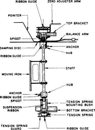
Friction torque, always a source of error, is due to imperfections in pivots and jewel bearings. Increasing use is now made of taut-band suspensions (Figure 11.2); this eliminates pivot friction and also replaces control springs. High-sensitivity moving-coil movements require only 0.005 mN-m for a 15 cm scale length: for moving-iron movements the torques are similar to those for the conventional pivoted instruments.
11.5.1.2 Scale shapes
The moving-coil instrument has a linear scale owing to the constant energy of the permanent magnet providing one of the two ‘force’ elements. All other classes of indicators are inherently of the double-energy type, giving a square-law scale of the linear property (voltage or current) being measured; for a wattmeter, the scale is linear for the average scalar product of voltage and current. The rectifier instrument, although an a.c. instrument, has a scale which is usually linear, as it depends on the moving-coil characteristic and the rectifier effect is usually negligible. (In low-range voltmeters, the rectifier has some effect and the scale shape is between linear and square law.) Thermal ammeters and electrodynamic voltmeters and ammeters usually have a true square-law scale, as any scale shaping requires extra torque and it is already low in these types. Moving-iron instruments are easily designed with high torque, and scale shaping is almost always carried out in order to approach a linear scale. In some cases the scale is actually contracted at the top in order to give an indication of overloads that would otherwise be off-scale. The best moving-iron scale shape is contracted only for about the initial 10% and is then nearly linear. Logarithmic scales have the advantage of equal percentage accuracy over all the scale, but they are difficult to read, owing to sudden changes in values of adjacent scale divisions. Logarithmic scales are unusual in switchboard instruments, but they are sometimes found in portable instruments, such as self-contained ohmmeters.
11.5.2 Direct voltage and current
11.5.2.1 Moving-coil indicator
This instrument comprises a coil, usually wound on a conducting former to provide eddy-current damping, with taut-band or pivot/control-spring suspension. In each case the coil rotates in the short air gap of a permanent magnet. The direction of the deflection depends on the polarity, so that unmodified indicators are usable only on d.c., and may have a centre zero if required. The error may be as low as ±0.1% of full-scale deflection; the range, from a few microamperes or millivolts up to 600 A and 750 V, which makes possible multirange d.c. test sets. The scale is generally linear (equispaced) and easily read. Non-linear scales can be obtained by shaping the magnet poles or the core to give a non-uniform air gap.
11.5.2.2 Corrections
The total power taken by a normal-range voltmeter can be 50 μW/V or more. For an ammeter the total series loss is 1–50 mW/A. Such powers may be a significant fraction of the total delivered to some electronic networks: in such cases electronic and digital voltmeters with trivial power loss should be used instead.
11.5.2.3 Induced moving-magnet indicator
The instrument is polarised by a fixed permanent magnet and so is only suitable for d.c. A small pivoted iron vane is arranged to lie across the magnet poles, the field of which applies the restoring torque. One or more turns of wire carry the current to be measured around the vane, producing a magnetic field at right angles to that of the magnet, and this drive torque deflects the movement to the equilibrium position. It is a cheap, low-accuracy instrument which can have a nearly linear centre-zero scale, well suited to monitoring battery charge conditions.
11.5.3 Alternating voltage and current
11.5.3.1 Moving-iron indicator
This is the most common instrument for a.c. at industrial frequency. Some (but not all) instruments may also be used on d.c. The current to be measured passes through a magnetising coil enclosing the movement. The latter is formed either from a nickel–iron alloy vane that is attracted into the field, or from two magnetic alloy members which, becoming similarly polarised, mutually repel. The latter is more usual but its deflection is limited to about 90°; however, when combined with attraction vanes, a 240° deflection is obtainable but can be used only on a.c. on account of the use of material of high hysteresis.
The inherent torque deflection is square law and so, in principle, the instrument measures true r.m.s. values. By careful shaping of vanes when made from modern magnetic alloys, a good linear scale has been achieved except for the bottom 10%, which readily distinguishes the instrument from the moving-coil linear scale. Damping torque is produced by eddy-current reaction in an aluminium disc moving through a permanent-magnet field.
11.5.3.2 Precautions and corrections
These instruments work at low flux densities (e.g. 7 mT), and care is necessary when they are used near strong ambient magnetic fields despite the magnetic shield often provided. As a result of the shape of the B/H curve, a.c./d.c. indicators used on a.c. read high at the lower end and low at the higher end of the scale. The effect of hysteresis with d.c. measurements is to make the ‘descending’ reading higher than the ‘ascending’.
Moving-iron instruments are available with class index values of 0.3–5.0, and many have similar accuracies for a.c. or d.c. applications. They tend to be single-frequency power instruments with a higher frequency behaviour that enables good r.m.s. readings to be obtained from supplies with distorted current waveforms, although excessive distortion will cause errors. Nevertheless, instruments can be designed for use in the lower audio range, provided that the power loss (a few watts) can be accepted. Ranges are from a few milliamperes and several volts upward. The power loss is usually significant and may have to be allowed for.
11.5.3.3 Electrodynamic indicator
In this the permanent magnet of the moving-coil instrument is replaced by an electromagnet (field coil). For ammeters the moving coil is connected in series with two fixed field coils; for voltmeters the moving and the fixed coils each have series-connected resistors to give the same time-constant, and the combination is connected in parallel across the voltage to be measured. With ammeters the current is limited by the suspension to a fraction of 1 A, and for higher currents it is necessary to employ non-reactive shunts or current transformers.
11.5.3.4 Precautions and corrections
The flux density is of the same order as that in moving-iron instruments, and similar precautions are necessary. The torque has a square-law characteristic and the scale is cramped at the lower end. By using the mean of reversed readings these instruments can be d.c. calibrated and used as adequate d.c./a.c. transfer devices for calibrating other a.c. instruments such as moving-iron indicators. The power loss (a few watts) may have to be allowed for in calculations derived from the readings.
11.5.3.5 Induction indicator
This single-frequency instrument is robust, but limited to class index (CI) number from 1.0 to 5.0. The current or voltage produces a proportional alternating magnetic field normal to an aluminium disc arranged to rotate. A second, phase-displaced field is necessary to develop torque. Originally it was obtained by pole ‘shading’, but this method is obsolete; modern methods include separate magnets one of which is shunted (Ockenden), a cylindrical aluminium movement (Lipman) or two electromagnets coupled by loops (Banner). The induction principle is most generally employed for the measurement of energy.
11.5.3.6 Moving-coil rectifier indicator
The place of the former copper oxide and selenium rectifiers has been taken by silicon diodes. Used with taut-band suspension, full-wave instrument rectifier units provide improved versions of the useful rectifier indicator.
11.5.3.7 Precautions and corrections
Owing to its inertia, the polarised moving-coil instrument gives a mean deflection proportional to the mean rectified current. The scale is marked in r.m.s. values on the assumption that the waveform of the current to be measured is sinusoidal with a form factor of 1.11. On non-sinusoidal waveforms the true r.m.s. value cannot be inferred from the reading: only the true average can be known (from the r.m.s. scale reading divided by 1.11). When true r.m.s. values are required, it is necessary to use a thermal, electrodynamic or square-law electronic instrument.
11.5.3.8 Multirange indicator
The rectifier diodes have capacitance, limiting the upper frequency of multirange instruments to about 20 kHz. The lower limit is 20–30 Hz, depending on the inertia of the movement. Indicators are available with CI numbers from 1.0 to 5.0, the multirange versions catering for a wide range of direct and alternating voltages and currents: a.c. 2.5V–2.5kV and 200 mA–10 A; d.c. 100 μV–2.5kV and 50 μA–10A. Non-linear resistance scales are normally included; values are derived from internal battery-driven out-of-balance bridge networks.
11.5.3.9 Moving-coil thermocouple indicator
The current to be measured (or a known proportion of it) is used as a heater current for the thermocouple, and the equivalent r.m.s. output voltage is steady because of thermal inertia–-except for very low frequency (5 Hz and below). With heater current of about 5 mA in a 100Ω resistor as typical, the possible voltage and current ranges are dictated by the usual series and shunt resistance, under the restriction that only the upper two-thirds of the square-law scale is within the effective range. The instrument has a frequency range from zero to 100 MHz. Normal radiofrequency (r.f.) low-range self-contained ammeters can be used up to 5 MHz with CI from 1.0 to 5.0. Instruments of this kind could be used in the secondary circuit of a r.f. current transformer for measurement of aerial current. The minimum measurable voltage is about 1 V.
The thermocouple, giving a true r.m.s. indication, is a primary a.c./d.c. transfer device. Recent evidence4 indicates that the transfer uncertainty is only a few parts in 106. Such devices provide an essential link in the traceability chain between microwave power, r.f. voltage and the primary standards of direct voltage and resistance.
11.5.3.10 Precautions and corrections
The response is slow, e.g. 5–10 s from zero to full-scale deflection, and the overload capacity is negligible: the heater may be destroyed by a switching surge. Thermocouple voltmeters are low-impedance devices (taking, e.g., 500 mW at 100 V) and may be unsuitable for electronic circuit measurements.
11.5.4 Medium and high direct and alternating voltage
11.5.4.1 Electrostatic voltmeter
This is in effect a variable capacitor with fixed and moving vanes. The power taken (theoretically zero) is in fact sufficient to provide the small dielectric loss. The basically square-law characteristic can be modified by shaping the vanes to give a reasonably linear upper scale. The minimum useful range is 50–150 V in a small instrument, up to some hundreds of kilovolts for large fixed instruments employing capacitor multipliers. Medium-voltage direct-connected voltmeters for ranges up to 15 kV have CI ratings from 1.0 to 5.0. The electrostatic indicator is a true primary alternating/direct voltage (a.v./d.v.) transfer device, but has now been superseded by the thermocouple instrument. The effective isolation property of the electrostatic voltmeter is attractive on grounds of safety for high-voltage measurements.
11.5.5 Power
11.5.5.1 Electrodynamic indicator
The instrument is essentially similar to the electrodynamic voltmeter and ammeter. It is usually ‘air-cored’, but ‘iron-cored’ wattmeters with high-permeability material to give a better torque/mass ratio are made with little sacrifice in accuracy. The current (fixed) coils are connected in series with the load, and the voltage (moving) coil with its series range resistor is connected either (a) across the load side of the current coil, or (b) across the supply side. In (a) the instrument reading must be reduced by the power loss in the volt coil circuit (typically 5 W), and in (b) by the current coil loss (typically 1 W).
The volt coil circuit power corrections are avoided by use of a compensated wattmeter, in which an additional winding in series with the volt circuit is wound, turn-for-turn, with the current coils, and the connection is (a) above. The m.m.f. due to the volt-coil circuit current in the compensating coil will cancel the m.m.f. due to the volt circuit current in the current coils.
The volt circuit terminal marked ± is immediately adjacent to the voltage coil; it should be connected to the current terminal similarly marked, to ensure that the wattmeter reads positive power and that negligible p.d. exists between fixed and moving coils, so safeguarding insulation and eliminating error due to electric torque.
When a wattmeter is used on d.c., the power should be taken from the mean of reversed readings; wattmeters read also the active (average) a.c. power. For the measurement of power at very low power factor, special wattmeters are made with weak restoring torque to give f.s.d. at, e.g., a power factor of 0.4. Range extension for all wattmeters on a.c. can be obtained by internal or external current transformers, internal resistive volt-range selectors or external voltage transformers. Typical self-contained ranges are between 0.5 and 20 A, 75 and 300 V. The usable range of frequency is about 30–150 Hz, with a best CI of 0.05.
Three-phase power can be measured by single dual-element instruments.
11.5.5.2 Thermocouple indicator
The modern versions of this instrument are more correctly termed electronic wattmeters. The outputs from current-and voltage-sensing thermocouples, multiplied together and amplified, can be displayed as average power. Typical d.c. and a.c. ranges are 300 mV–300V and 10 mA–10 A, from pulsed and other non-sinusoidal sources at frequencies up to a few hundred kilohertz. The interaction with the network is low; e.g. the voltage network has typically an impedance of 10 k Ω/V.
11.5.6 Maximum alternating current
11.5.6.1 Maximum-demand instrument
The use of an auxiliary pointer carried forward by the main pointer and remaining in position makes possible the indication of maximum current values, but the method is not satisfactory, because it demands large torques, a condition that reduces effective damping and gives rise to overswing. A truer maximum demand indication, and one that is insensitive to momentary peaks, is obtainable with the aid of a thermal bimetal. Passing the current to be indicated through the bimetal gives a thermal lag of a few minutes. For long-period indication (1 h or more) a separate heater is required.
Such instruments have been adapted for three-phase operation using separate heaters. A recent development permits a similar device to be used for two phases of a three-phase supply. The currents are summed linearly, and the maximum of the combined unbalanced currents maintained for 45 min is recorded on a kV-A scale marked in terms of nominal voltage.
11.5.7 Power factor
Power factor indicators have both voltage and current circuits, and can be interconnected to form basic electrodynamic or moving-iron direct-acting indicators. The current coils are fixed; the movement is free, the combined voltage-and current-excited field producing both deflecting and controlling torque. The electrodynamic form has the greater accuracy, but is restricted to a 90° deflection, as compared with 360° (90° lag and lead, motoring and generating) of the moving-iron type.
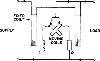
One electrodynamic form comprises two fixed coils carrying the line current, and a pair of moving volt coils set with their axes mutually at almost 90° (Figure 11.3). For one-phase operation the volt-coil currents are nearly in quadrature, being, respectively, connected in series with an inductor L and a resistor R. For three-phase working, L is replaced by a resistor r and the ends of the volt-coil circuits taken, respectively, to the second and third phases. A three-phase moving-iron instrument for balanced loads has one current coil and three volt coils (or three current and one voltage); if the load is unbalanced, three current and three volt coils are required. All these power factor indicators are industrial frequency devices.
The one-phase electrodynamic wattmeter can be used as a phase-sensing instrument. When constant r.m.s. voltages and currents from two, identical-frequency, sinusoidal power supplies are applied to the wattmeter, then the phase change in one system produces power scale changes which are proportional to cos φ.
Many electronic phase-meters of the analogue and digital type are available which, although not direct-acting, have high impedance inputs, and they measure the phase displacement between any two voltages (of the same frequency) over a wide range of frequencies. Either the conventional solid state digital instruments generate a pulse when the two voltages pass zero, and measure and display the time between these pulses as phase difference, or the pulses trigger a multivibrator for the same period, to generate an output current proportional to phase (time) difference. These instruments provide good discrimination and, with modern high-speed logic switching, the instant for switch-on (i.e. pulse generation) is less uncertain: conversely, the presence of small harmonic voltages around zero could lead to some ambiguity.
11.5.8 Phase sequence and synchronism
A small portable form of phase sequence indicator is essentially a primitive three-phase induction motor with a disc rotor and stator phases connected by clip-on leads to the three-phase supply. The disc rotates in the marked forward direction if the sequence is correct. These instruments have an intermittent rating and must not be left in circuit.
The synchroscope is a power factor instrument with rotor slip-rings to allow continuous rotation. The moving-iron type is robust and cheap. The direction of rotation of the rotor indicates whether the incoming three-phase system is ‘fast’ or ‘slow’, and the speed of rotation measures the difference in frequency.
11.5.9 Frequency
Power frequency monitoring frequency indicators are based on the response of reactive networks. Both electrodynamic and induction instruments are available, the former having the better accuracy, the latter having a long scale of 300° or more.
One type of indicator consists of two parallel fixed coils tuned to slightly different frequencies, and their combined currents return to the supply through a moving coil which lies within the resultant field of the fixed coils. The position of the moving coil will be unique for each frequency, as the currents (i.e. fields) of the fixed coils are different unique functions of frequency. The indications are within a restricted range of a few hertz around nominal frequency. A ratiometer instrument, which can be used up to a few kilohertz, has a permanent-magnet field in which lie two moving coils set with their planes at right angles. Each coil is driven by rectified a.c, through resistive and capacitive impedances, respectively, and the deflection is proportional to frequency.
Conventional solid state counters are versatile time and frequency instruments. The counter is based on a stable crystal reference oscillator (e.g. at 1 MHz) with an error between 1 and 10 parts in 108 per day. The displays have up to eight digits, with a top frequency of 100 MHz (or 600 MHz with heterodyning). The resolution can be 10 ns, permitting pulse widths of 1000 ns to be assessed to 1%: but a 50 Hz reading would be near to the bottom end of the display, giving poor discrimination. All counters provide for measurements giving the period of a waveform to a good discrimination.
11.6 Integrating (energy) metering
Integrating meters record the time integral of active, reactive and apparent power as a continuous summation. The integration may be limited by a specified total energy (e.g. prepayment meters) or by time (e.g. maximum demand). Meters for a.c. supplies are all of the induction type, with measuring elements in accordance with the connection of the load (one-phase or three- or four-wire three-phase). Manufacturing and testing specifications are given in BS 37. Instrument transformers for use with meters are listed in BS 3938 and BS 3941.
11.6.1 Single-phase meter
The rotor is a light aluminium disc on a vertical spindle, supported in low-friction bearings. The lower bearing is a sapphire cup, carrying the highly polished hemispherical hardened steel end of the spindle. The rotor is actuated by an induction driving element and its speed is controlled by an eddy current brake. The case is usually a high-quality black phenolic moulding with integral terminal block. The frame is a rigid high-stability iron casting which serves as the mounting, as part of a magnetic flux path, and as a shield against ambient magnetic fields.
The driving element has the basic form shown in Figure 11.4. It has two electromagnets, one voltage-excited and the other current-excited. The volt magnet, roughly of E-shape, has a nearly complete magnetic circuit with a volt coil on the central limb. Most of the flux divides between the outer limbs, but the working flux from the central limb penetrates the disc and enters the core of the current magnet. The latter, of approximate U-shape, is energised by a coil carrying the load current. With a condition of zero load current, the working flux from the volt magnet divides equally between the two limbs of the current magnet and returns to the volt magnet core through the frame, or through an iron path provided for this purpose. If the volt magnet flux is symmetrically disposed, the eddy current induced in the disc does not exert any net driving torque and the disc remains stationary. The volt magnet flux is approximately in phase quadrature with the applied voltage.
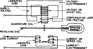
When a load current flows in the coil of the current magnet, it develops a co-phasal flux, interacting with the volt magnet flux to produce a resultant that ‘shifts’ from one current magnet pole to the other. Force is developed by interaction of the eddy currents in the disc and the flux in which it lies, and the net torque is proportional to the voltage and to that component of the load current in phase with the voltage—i.e. to the active power. The disc therefore rotates in the direction of the ‘shift’.
The disc rotates through the field of a suitably located permanent isotropic brake magnet, and induced currents provide a reaction proportional to speed. Full-load adjustment is effected by means of a micrometer screw which can set the radial position of the brake magnet.
The volt magnet working flux lags the voltage by a phase angle rather less than 90° (e.g. by 85°). The phase angle is made 90° by providing a closed quadrature coil on the central limb, with its position (or resistance) capable of adjustment.
The accuracy of the meter is affected on low loads by pivot friction. A low-load adjustment, consisting of some device that introduces a slight asymmetry in the volt magnet working flux, is fitted to mitigate frictional error. There are several methods of producing the required asymmetry: one is the insertion of a small magnetic vane into the path of the working flux. The asymmetry results in the development at zero load of a small forward torque, just sufficient to balance friction torque without causing the disc to rotate.
11.6.1.1 Performance of single-phase meters
The limits of permissible error are defined in BS 37. In general, the error should not exceed ± 2% over most of the working range for credit meters. For prepayment meters, +2 and −3% for loads above 1/30 full load at unity power factor, at any price setting to be used, are the specified limits. Tests for compliance with this requirement at and below 1/10 marked current must be made with the coin condition that not less than one nor more than three coins of the highest denomination acceptable by the meter are prepaid.
It is usual for manufacturers to adjust their meters to less than one-half of the permissible error over much of the working range. The mean error of an individual meter is, of course, less than the maximum observable error, and the mean collective error of a large number of meters is likely to be much less than ± 1% at rated voltage and frequency. If no attempt is made during production testing to bias the error in one direction, the weighted mean error of many meters taken collectively is probably within 0.5%, and is likely to be positive (see Figure 11.5(a)).

11.6.1.2 Temperature
The temperature error of a.c. meters with no temperature compensation is negligible under the conditions normally existing in the UK. In North America it is common practice to fix meters on the outside of buildings, where they are subjected to wide temperature ranges (e.g. 80°C), which makes compensation desirable. However, even in the UK it is common to provide compensation (when required) in the form of a strip of nickel-rich alloy encircling the stator magnet. Its use is advantageous for short-duration testing, as there is an observable difference in error of a meter when cold and after a 30 min run.
11.6.1.3 Voltage and frequency
Within the usual limits of ± 4% in voltage and ± 0.2% in frequency, the consequent errors in a meter are negligible. Load-shedding, however, may mean substantial reductions of voltage and frequency. A significant reduction in voltage usually causes the meter to read high on all loads, as shown in Figure 11.5(b). Reduction of the supply frequency makes the meter run faster on high-power-factor loads and slower on lagging reactive loads: an increase of frequency has the opposite effect (Figure 11.5)(c). The errors are cumulative if both voltage and frequency variations occur together.
11.7 Electronic instrumentation
The rapid development of large-scale integrated (l.s.i.) circuits, as applied to analogue and especially digital circuitry, has allowed both dramatic changes in the format of measurement instrumentation by designers and in the measurement test systems available for production or control applications.
A modern instrument is often a multipurpose assembly, including a microprocessor for controlling both the sequential measurement functions and the subsequent programmed assessment of the data retained in its store; hence, these instruments can be economical in running and labour costs by avoiding skilled attention in the recording and statistical computation of the data. Instruments are often designed to be compatible with standardised interfaces, such as the IEC bus or IEEE-488 bus, to form automatic measurement systems for interactive design use of feedback digital-control applications; typically a system would include a computer-controlled multiple data logger with 30 inputs from different parameter sensors, statistical and system analysers, displays and storage. The input analogue parameters would use high-speed analogue-to-digital (A/D) conversion, so minimising the front-end analogue conditioning networks while maximising the digital functions (e.g. filtering and waveform analyses by digital rather than analogue techniques). The readout data can be assembled digitally and printed out in full, or presented through D/A converters in graphical form on X–Y plotters using the most appropriate functional co-ordinates to give an economical presentation of the data.
The production testing of the component subsystems in the above instruments requires complex instrumentation and logical measurements, since there are many permutations of these minute logic elements resulting in millions of high-speed digital logic operations—which precludes a complete testing cycle, owing to time and cost. Inspection testing of l.s.i. analogue or digital devices and subassemblies demands systematically programmed measurement testing sequences with varied predetermined signals; similar automatic test equipments (ATE) are becoming more general in any industrial production line which employs these modern instruments in process or quality-control operations. Some companies are specialising in computer-orientated measurement techniques to develop this area of ATE; economic projections indicate that the present high growth rate in ATE-type measurement systems will continue or increase during the next few years.
The complementary nature of automated design, production and final testing types of ATE leads logically to the interlinking of these separate functions for optimising and improving designs within the spectrum of production, materials handling, quality control and costing to provide an overall economic and technical surveillance of the product.
Some of the more important instruments have been included in the survey of electronic instrumentation in the following pages, but, owing to the extensive variety of instruments at present available and the rapid rate of development in this field, the selection must be limited to some of the more important devices.
Digital instruments usually provide an output in visual decimal or coded digit form as a discontinuous function of a smoothly changing input quantity. In practice the precision of a digital instrument can be extended by adding digits to make it better than an analogue instrument, although the final (least significant) digit must always be imprecise to ± 0.5.
11.7.1 Digital voltmeters
These provide a digital display of d.c. and/or a.c. inputs, together with coded signals of the visible quantity, enabling the instrument to be coupled to recording or control systems. Depending on the measurement principle adopted, the signals are sampled at intervals over the range 2–500 ms. The basic principles are: (a) linear ramp; (b) charge balancing; (c) successive-approximation/potentiometric; (d) voltage to frequency integration; (e) dual slope; (f) multislope; and (g) some combination of the foregoing.
Modern digital voltmeters often include a multiway socket connection (e.g. BCD; IEC bus; IEEE-488 bus, etc.) for data/interactive control applications.
11.7.1.1 Linear ramp
This is a voltage/time conversion in which a linear time-base is used to determine the time taken for the internally generated voltage vs to change by the value of the unknown voltage V. The block diagram (Figure 11.6(b)) shows the use of comparison networks to compare V with the rising (or falling) vs; these networks open and close the path between the continuously running oscillator, which provides the counting pulses at a fixed clock rate, and the counter. Counting is performed by one of the binary-coded sequences; the translation networks give the visual decimal output. In addition, a binary-coded decimal output may be provided for monitoring or control purposes.

Limitations are imposed by small non-linearities in the ramp, the instability of the ramp and oscillator, imprecision of the coincidence networks at instants y and z, and the inherent lack of noise rejection. The overall uncertainty is about ±0.05% and the measurement cycle would be repeated every 200 ms for a typical four-digit display.
Linear ‘staircase’ ramp instruments are available in which V is measured by counting the number of equal voltage ‘steps’ required to reach it. The staircase is generated by a solid state diode pump network, and linearities and accuracies achievable are similar to those with the linear ramp.
11.7.1.2 Charge balancing
This principle5 employs a pair of differential-input transistors used to charge a capacitor by a current proportional to the unknown d.c. voltage, and the capacitor is then discharged by a large number of small +δq and -δq quantities, the elemental discharges being sensed and directed by fast comparator/flip-flop circuits and the total numbers being stored. Zero is in the middle of the measurement range and the displayed result is proportional to the difference between the number of +δq, -δq events.
The technique which, unlike dual-ramp methods, is inherently bipolar, claims some other advantages, such as improved linearity, more rapid recovery from overloads, higher sensitivity and reduced noise due to the averaging of thousands of zero crossings during the measurement, as well as a true digital auto-zero subtraction from the next measurement, as compared with the more usual capacitive-stored analogue offset p.d. being subtracted from the measured p.d.
Applications of this digital voltmeter system (which is available on a monolithic integrated circuit, Ferranti ZN 450) apart from d.c. and a.c. multimeter uses, include interfacing it directly with a wide range of conventional transducers such as thermocouples, strain gauges, resistance thermometers, etc.
11.7.1.3 Successive approximation
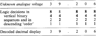
As it is based on the potentiometer principle, this class produces very high accuracy. The arrows in the block diagram of Figure 11.7 show the signal-flow path for one version; the resistors are selected in sequence so that, with a constant current supply, the test voltage is created within the voltmeter.

Each decade of the unknown voltage is assessed in terms of a sequence of accurate stable voltages, graded in descending magnitude in accordance with a binary (or similar) counting scale. After each voltage approximation of the final result has been made and stored, the residual voltage is then automatically re-assessed against smaller standard voltages, and so on to the smallest voltage discrimination required in the result. Probably four logic decisions are needed to select the major decade value of the unknown voltage, and this process will be repeated for each lower decade in decimal sequence until, after a few milliseconds, the required voltage is stored in a coded form. This voltage is then translated for decimal display. A binary-coded sequence could be as shown in Table 11.2, where the numerals in bold type represent a logical rejection of that number and a progress to the next lower value. The actual sequence of logical decisions is more complicated than is suggested by the example. It is necessary to sense the initial polarity of the unknown signal, and to select the range and decimal marker for the read-out; the time for the logic networks to settle must be longer for the earlier (higher voltage) choices than for the later ones, because they must be of the highest possible accuracy; offset voltages may be added to the earlier logic choices, to be withdrawn later in the sequence; and so forth.
The total measurement and display takes about 5 ms. When noise is present in the input, the necessary insertion of filters may extend the time to about 1 s. As noise is more troublesome for the smaller residuals in the process, it is sometimes convenient to use some different techniques for the latter part. One such is the voltage–frequency principle (see below), which has a high noise rejection ratio. The reduced accuracy of this technique can be tolerated as it applies only to the least significant figures.
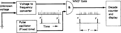
11.7.1.4 Voltage–frequency
The converter (Figure 11.8) provides output pulses at a frequency proportional to the instantaneous unknown input voltage, and the non-uniform pulse spacing represents the variable frequency output. The decade counter accumulates the pulses for a predetermined time T and in effect measures the average frequency during this period. When T is selected to coincide with the longest period time of interfering noise (e.g. mains supply frequency), such noise averages out to zero.
Instruments must operate at high conversion frequencies if adequate discrimination is required in the final result. If a six-digit display were required within 5 ms for a range from zero to 1.000 00 V to ± 0.01%, then 105 counts during 5 ms are called for, i.e. a 20 MHz change from zero frequency with a 0.01% voltage–frequency linearity. To reduce the frequency range, the measuring time is increased to 200 ms or higher. Even at the more practical frequency of 0.5 MHz that results, the inaccuracy of the instrument is still determined largely by the non-linearity of the voltage–frequency conversion process.
In many instruments the input network consists of an integrating operational amplifier in which the average input voltage is ‘accumulated’ in terms of charge on a capacitor in a given time.
11.7.1.5 Dual-slope
This instrument uses a composite technique consisting of an integration (as mentioned above) and an accurate measuring network based on the ramp technique. During the integration (Figure 11.9) the unknown voltage Vx is switched at time zero to the integration amplifier, and the initially uncharged capacitor C is charged to Vx in a known time T1, which may be chosen so as to reduce noise interference. The ramp part of the process consists in replacing Vx by a reversed biased direct reference voltage Vr which produces a constant-current discharge of C; hence, a known linear voltage/time change occurs across C. The total voltage change to zero can be measured by the method used in the linear-ramp instrument, except that the slope is negative and that counting begins at maximum voltage. From the diagram in Figure 11.9(a) it follows that tan θx/tan θr = (T2 − T1)/T1 = Vx/Vr so that Vx is directly proportional to T2−T1. The dual-slope method is seen to depend ultimately on time-base linearity and on the measurement of time difference, and is subject to the same limitations as the linear-ramp method, but with the important and fundamental quality of inherent noise rejection capability.
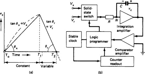
Noise interference (of series-mode type) is principally due to e.m.f.s at power supply frequency being induced into the d.c. source of Vx. When T1 equals the periodic time of the interference (20 ms for 50 Hz), the charging p.d. vc across C would follow the dotted path (Figure 11.9(a)) without changing the final required value of vc, thus eliminating this interference.
11.7.1.6 Multislope
At time T1 (above) the maximum dielectric absorption in C will coincide with vc maximum; this effect degrades (a) the linearity of the run-down slope during T2 − T1 and (b) the identification of zero p.d. One improved ‘multislope’ technique reduces dielectric absorption in C by inserting various reference voltages during the run-up period and, after subtraction, leaves a lower p.d., v′c, prior to run-down while storing the most significant digit of Vx during the run-up period. During run-down, C is discharged rapidly to measure the next smaller digit; the residue of v′c, including overshoot, is assessed to give the remaining three digits in sequence using three vr/t functions of slope +1/10, −1/100, + 1/1000 compared with the initial rapid discharge. Measurement time is reduced, owing to the successive digits being accumulated during the measurement process.6
11.7.1.7 Mixed techniques
Several techniques can be combined in the one instrument in order to exploit to advantage the best features of each. One accurate, precise, digital voltmeter is based upon precision inductive potentiometers, successive approximation, and the dual-slope technique for the least significant figures. An uncertainty of 10 parts in 106 for a 3-month period is claimed, with short-term stability and a precision of about 2 parts in 106.
11.7.1.8 Digital multimeters
Any digital voltmeter can be scaled to read d.c. or a.c. voltage, current, immittance or any other physical property, provided that an appropriate transducer is inserted. Instruments scaled for alternating voltage and current normally incorporate one of the a.c./d.c. converter units listed in a previous paragraph, and the quality of the result is limited by the characteristics inherent in such converters. The digital part of the measurement is more accurate and precise than the analogue counterpart, but may be more expensive.
For systems application, programmed signals can be inserted into, and binary-coded or analogue measurements received from, the instrument through multiway socket connections, enabling the instrument to form an active element in a control system (e.g. IEC bus, IEEE-488 bus).
Resistance, capacitance and inductance measurements depend to some extent on the adaptability of the basic voltage-measuring process. The dual-slope technique can be easily adapted for two-, three- or four-terminal ratio measurements of resistance by using the positive and negative ramps in sequence; with other techniques separate impedance units are necessary. (See Table 11.3)
Table 11.3
Typical characteristics of digital multimeters

*Specifications often include 12-, 6-, and 3-month periods each with progressively smaller uncertainties of measurement down to 24-h statements for high precision instruments.
11.7.1.9 Input and dynamic impedance
The high precision and small uncertainty of digital voltmeters make it essential that they have a high input impedance if these qualities are to be exploited. Low test voltages are often associated with source impedances of several hundred kilo-ohms; for example, to measure a voltage with source resistance 50 k Ω to an uncertainty of ±0.005% demands an instrument of input resistance 1 G Ω, and for a practical instrument this must be 10 G Ω if the loading error is limited to one-tenth of the total uncertainty.
The dynamic impedance will vary considerably during the measuring period, and it will always be lower than the quoted null, passive, input impedance. These changes in dynamic impedance are coincident with voltage ‘spikes’ which appear at the terminals owing to normal logic functions; this noise can adversely affect components connected to the terminals, e.g. Weston standard cells.
Input resistances of the order of 1–10 G Ω represent the conventional range of good-quality insulators. To these must be added the stray parallel reactance paths through unwanted capacitive coupling to various conducting and earth planes, frames, chassis, common rails, etc.
11.7.1.10 Noise limitation
The information signal exists as the p.d. between the two input leads; but each lead can have unique voltage and impedance conditions superimposed on it with respect to the basic reference or ground potential of the system, as well as another and different set of values with respect to a local earth reference plane.
An elementary electronic instrumentation system will have at least one ground potential and several earth connections–-possibly through the (earthed) neutral of the main supply, the signal source, a read-out recorder or a cathode ray oscilloscope. Most true earth connections are at different electrical potentials with respect to each other, owing to circulation of currents (d.c. to u.h.f.) from other apparatus, through a finite earth resistance path. When multiple earth connections are made to various parts of a high-gain amplifier system, it is possible that a significant frequency spectrum of these signals will be introduced as electrical noise. It is this interference which has to be rejected by the input networks of the instrumentation, quite apart from the concomitant removal of any electrostatic/electromagnetic noise introduced by direct coupling into the signal paths. The total contamination voltage can be many times larger (say 100) than the useful information voltage level.
Electrostatic interference in input cables can be greatly reduced by ‘screened’ cables (which may be 80% effective as screens), and electromagnetic effects minimised by transposition of the input wires and reduction in the ‘aerial loop’ area of the various conductors. Any residual effects, together with the introduction of ‘ground and earth-loop’ currents into the system, are collectively referred to as series and/or common-mode signals.
11.7.1.11 Series and common-mode signals
Series-mode (normal) interference signals, Vsm, occur in series with the required information signal. Common-mode interference signals, Vcm, are present in both input leads with respect to the reference potential plane: the required information signal is the difference voltage between these leads. The results are expressed as rejection ratio (in decibels) with respect to the effective input error signal, Ve, that the interference signals produce, i.e.
where K is the rejection ratio. The series-mode rejection networks are within the amplifier, so Vc is measured with zero normal input signal as Ve = output interference voltage ÷ gain of the amplifier appropriate to the bandwidth of Ve.
Consider the elementary case in Figure 11.10, where the input-lead resistances are unequal, as would occur with a transducer input. Let r be the difference resistance, C the cable capacitance, with common-mode signal and error voltages Vcm and Ve, respectively. Then the common-mode numerical ratio (c.m.r.) is

assuming the cable insulation to be ideal, and XC ![]() r. Clearly, for a common-mode statement to be complete, it must have a stated frequency range and include the resistive imbalance of the source. (It is often assumed in c.m.r. statements that r = 1 k Ω.)
r. Clearly, for a common-mode statement to be complete, it must have a stated frequency range and include the resistive imbalance of the source. (It is often assumed in c.m.r. statements that r = 1 k Ω.)
The c.m.r. for a digital voltmeter could be typically 140dB (corresponding to a ratio of 107/1) at 50 Hz with a 1 k Ω line imbalance, and leading consequently to C = 0.3 pF. As the normal input cable capacitance is of the order of 100 pF/m, the situation is not feasible. The solution is to inhibit the return path of the current i by the introduction of a guard network. Typical guard and shield parameters are shown in Figure 11.11 for a six-figure digital display on a voltmeter with ± 0.005% uncertainty. Consider the magnitude of the common-mode error signal due to a 5 V, 50 Hz common-mode voltage between the shield earth E1 and the signal earth E2:

11.7.1.12 Floating-voltage measurement
If the d.c. voltage difference to be measured has a p.d. to E2 of 100 V, as shown, then with N–G open the change in p.d. across r will be 50 μV, as a series-mode error of 0.005% for a 1 V measurement. With N–G connected the change will be 1 μV, which is negligible.
The interconnection of electronic apparatus must be carefully made to avoid systematic measurement errors (and short circuits) arising from incorrect screen, ground or earth potentials.
In general, it is preferable, wherever possible, to use a single common reference node, which should be at zero signal reference potential to avoid leakage current through r. Indiscriminate interconnection of the shields and screens of adjacent components can increase noise currents by short-circuiting the high-impedance stray path between the screens.
11.7.1.13 Instrument selection
A precise seven-digit voltmeter, when used for a 10 V measurement, has a discrimination of ±1 part in 106 (i.e. ±10μV), but has an uncertainty (‘accuracy’) of about ±10 parts in 106 (i.e. ±100 μV). The distinction is important with digital read-out devices, lest a higher quality be accorded to the number indicated than is in fact justified. The quality of any reading must be based upon the time stability of the total instrument since it was last calibrated against external standards, and the cumulative evidence of previous calibrations of a like kind.
Selection of a digital voltmeter from the list of types given in Table 11.3 is based on the following considerations:
(1) No more digits than necessary, as the cost per extra digit is high.
(2) High input impedance, and the effect on likely sources of the dynamic impedance.
(3) Electrical noise rejection, assessed and compared with (a) the common-mode rejection ratio based on the input and guard terminal networks and (b) the actual inherent noise rejection property of the measuring principle employed.
(4) Requirements for binary-coded decimal, IEEE-488, storage and computational facilities.
(5) Versatility and suitability for use with a.c. or impedance converter units.
(6) Use with transducers (in which case (3) is the most important single factor).
11.7.1.14 Calibration
It will be seen from Table 11.3 that digital voltmeters should be recalibrated at intervals between 3 and 12 months. Built-in self-checking facilities are normally provided to confirm satisfactory operational behaviour, but the ‘accuracy’ check cannot be better than that of the included standard cell or Zener diode reference voltage and will apply only to one range. If the user has available some low-noise stable voltage supplies (preferably batteries) and some high-resistance helical voltage dividers, it is easy to check logic sequences, resolution, and the approximate ratio between ranges. In order to demonstrate traceability to national standards, a voltage source whose voltage is traceable to national standards should be used. This can either be done by the user or, more commonly, by sending the instrument to an accredited calibration laboratory.
11.7.2 Digital wattmeters7–9
Digital wattmeters employ various techniques for sampling the voltage and current waveforms of the power source to produce a sequence of instantaneous power representations from which the average power is obtained. One new NPL method uses high-precision successive-approximation A/D integrated circuits with the multiplication and averaging of the digitised outputs being completed by computer.10,11 A different ‘feedback time-division multiplier’ principle is employed by Yokogawa Electric Limited.r
The NPL digital wattmeter uses ‘sample and hold’ circuits to capture the two instantaneous voltage (vx) and current (ix) values, then it uses a novel double dual-slope multiplication technique to measure the average power from the mean of numerous instantaneous (vxix) power measurements captured at precise intervals during repetitive waveforms. Referring to the single dual-ramp (Figure 11.9(a)) the a.c. voltage vx (captured at T0) is measured as vxT1 = Vr(T2 – T1). If a second voltage (also captured at T0) is proportional to ix and integrated for T2 – T1, then, if it is reduced to zero (by Vr) during the time T3 – T2 it follows that ix(T2 – T1) = Vr(T3 − T2).
The instantaneous power (at T0) is vxix = K(T3 – T2) and, by scaling, the mean summation of all counts such as T3 – T2 equals the average power. The prototype instrument measures power with an uncertainty of about ±0.03% f.s.d. (and ±0.01%, between 50 and 400 Hz, should be possible after further development).
The ‘feedback time division multiplier’ technique develops rectangular waveforms with the pulse height and width being proportional, respectively, to the instantaneous voltage (vx) and current (ix); the average ‘area’ of all such instantaneous powers (vxix) is given (after 1.p. filtering) as a d.c. voltage measured by a DVM scaled in watts; such precision digital wattmeters, operating from 50 to 500 Hz, have ±0.05% to ±0.08% uncertainty for measurements up to about 6kW.
11.7.3 Energy meters
A solid state single-phase meter is claimed to fulfil the specifications of its traditional electromechanical counterpart while providing a reduced uncertainty of measurement coupled with improved reliability at a similar cost. The instrument should provide greater flexibility for reading, tariff and data communication of all kinds, e.g. instantaneous power information, totalised energy, credit limiting and multiple tariff control. The instrument is less prone to fraudulent abuse.
11.7.4 Signal generators
Signal generators provide sinusoidal, ramp and square-wave output from fractions of 1 Hz to a few megaherz, although the more accurate and stable instruments generally cover a more restricted range. As voltage sources, the output power is low (100 mW–2W). The total harmonic distortion (i.e. r.m.s. ratio between harmonic voltage and fundamental voltage) must be low, particularly for testing-quality amplifiers, e.g. 90 dB rejection is desirable and 60 dB (103:1) is normal for conventional oscillators. Frequency selection by dials may introduce ±2% uncertainty, reduced to 0.2% with digital dial selection which also provides 0.01% reproducibility. Frequency-synthesiser function generators should be used when a precise, repeatable frequency source is required. Amplitude stability and constant value over the whole frequency range is often only 1–2% for normal oscillators.
11.7.5 Electronic analysers
Analysers include an important group of instruments which operate in the frequency domain to provide specialised analyses, in terms of energy, voltage, ratio, etc., (a) to characterise networks, (b) to decompose complex signals which include analogue or digital intelligence, and (c) to identify interference effects and non-linear cross-modulations throughout complex systems.
The frequency components of a complex waveform (Fourier analysis) are selected by the sequential, or parallel, use of analogue to digital filter networks. A frequency-domain display consists of the simultaneous presentation of each separate frequency component, plotted in the x-direction to a base of frequency, with the magnitude of the y-component representing the parameter of interest (often energy or voltage scaled in decibels).
Instruments described as network, signal, spectrum or Fourier analysers as well as digital oscilloscopes have each become so versatile, with various built-in memory and computational facilities, that the distinction between their separate objectives is now imprecise. Some of the essential generic properties are discussed below.
11.7.5.1 Network analysers
Used in the design and synthesis of complex cascaded networks and systems. The instrument normally contains a swept-frequency sinusoidal source which energises the test system and, using suitable connectors or transducers to the input and output ports of the system, determines the frequency-domain characteristic in ‘lumped’ parameters and the transfer function equations in both magnitude and phase: high-frequency analysers often characterise networks in ‘distributed’ s-parameters for measurements of insertion loss, complex reflection coefficients, group delay, etc. Three or four separate instruments may be required for tests up to 40 GHz. Each instrument would have a wide dynamic range (e.g. 100 dB) for frequency and amplitude, coupled with high resolution (e.g. 0.1 Hz and 0.01 dB) and good accuracy, often derived from comparative readings or ratios made from a built-in reference measurement channel.
Such instruments have wide applications in research and development laboratories, quality control and production testing–-and they are particularly versatile as an automatic measurement testing facility, particularly when provided with built-in programmable information and a statistical storage capability for assessment of the product. Data display is by X – Y recorder and/or cathode-ray oscilloscope (c.r.o.) and the time-base is locked to the swept frequency.
11.7.5.2 Spectrum analysers
Spectrum analysers normally do not act as sources; they employ a swept-frequency technique which could include a very selective, narrow-bandwidth filter with intermediate frequency (i.f.) signals compared, in sequence, with those selected from the swept frequency; hence, close control of frequency stability is needed to permit a few per cent resolution within, say, a 10 Hz bandwidth filter. Instruments can be narrow range, 0.1 Hz–30 kHz, up to wide range, 1 MHz–40 GHz, according to the precision required in the results; typically, an 80 dB dynamic range can have a few hertz bandwidth and 0.5 dB amplitude accuracy. Phase information is not directly available from this technique. The instrument is useful for tests involving the output signals from networks used for frequency mixing, amplitude and frequency modulation or pulsed power generation. A steady c.r.o. display is obtained from the sequential measurements owing to digital storage of the separate results when coupled with a conventional variable-persistence cathode-ray tube (a special cathode-ray tube is not required for a digital oscilloscope): the digitised results can, in some instruments, be processed by internal programs for (a) time averaging of the input parameters, (b) probability density and cumulative distribution, and (c) a comprehensive range of statistical functions such as average power or r.m.s. spectrum, coherence, autocorrelation and cross-correlation functions, etc.
11.7.5.3 Fourier analysers
Fourier analysers use digital signalling techniques to provide facilities similar to the spectrum analysers but with more flexibility. These ‘Fourier’ techniques are based upon the calculation of the discrete Fourier transform using the fast Fourier transform algorithm (which calculates the magnitude and phase of each frequency component using a group of time-domain signals from the input signal variation of the sampling rate); it enables the long measurement time needed for very-low-frequency (![]() 1 Hz) assessments to be completed in a shorter time than that for a conventional swept measurement—together with good resolution (by digital translation) at high frequencies. Such specialised instruments are usable only up to 100 kHz but they are particularly suitable for examining low-frequency phenomena such as vibration, noise transmission through media and the precise measurement of random signals obscured by noise, etc.
1 Hz) assessments to be completed in a shorter time than that for a conventional swept measurement—together with good resolution (by digital translation) at high frequencies. Such specialised instruments are usable only up to 100 kHz but they are particularly suitable for examining low-frequency phenomena such as vibration, noise transmission through media and the precise measurement of random signals obscured by noise, etc.
11.7.6 Data loggers
Data loggers consist of an assembly of conditioning amplifiers which accept signals from a wide range of transducers or other sources in analogue or digital form; possibly a small computer program will provide linearisation and other corrections to signals prior to computational assessments (comparable to some features of a spectrum or other class of analyser) before presenting the result in the most economical manner (such as a graphical display). The data logger, being modular in construction, is very flexible in application; it is not limited to particular control applications and by the nature of the instrument can appear in various guises.
11.8 Oscilloscopes
The cathode-ray oscilloscope (c.r.o.) is one of the most versatile instruments in engineering. It is used for diagnostic testing and monitoring of electrical and electronic systems, and (with suitable transducers) for the display of time-varying phenomena in many branches of physics and engineering. Two-dimensional functions of any pair of repetitive, transient or pulse signals can be developed on the fluorescent screen of a c.r.o.
These instruments may be classified by the manner in which the analogue test signals are conditioned for display as (a) the ‘analogue c.r.o.’, using analogue amplifiers, and (b) the ‘digital storage oscilloscope’, using A/D converters at the input with ‘all-digit’ processing.
11.8.1 Cathode-ray tube
The cathode-ray tube takes its name from Pluecker’s discovery in 1859 of ‘cathode rays’ (a better name would be ‘electron beam’, for J. J. Thomson in 1897 showed that the ‘rays’ consist of high-speed electrons). The developments by Braun, Dufour and several other investigators enabled Zworykin in 1929 to construct the essential features of the modern cathode-ray tube, namely a small thermionic cathode, an electron lens and a means for modulating the beam intensity. The block diagram (Figure 11.12) shows the principal components of a modern cathode-ray oscilloscope. The tube is designed to focus and deflect the beam by means of structured electric field patterns. Electrons are accelerated to high speed as they travel from the cathode through a potential rise of perhaps 15kV. After being focused, the beam may be deflected by two mutually perpendicular X and Y electric fields, locating the position of the fluorescing ‘spot’ on the screen.

11.8.1.1 Electron gun and beam deflection
The section of the tube from which the beam emerges includes the heater, cathode, grid and the first accelerating anode; these collectively form the electron gun. A simplified diagram of the connections is given in Figure 11.13. The electric field of the relatively positive anode partly penetrates through the aperture of the grid electrode and determines on the cathode a disc-shaped area (bounded by the −15 kV equipotential) within which electrons are drawn away from the cathode: outside this area they are driven back. With a sufficiently negative grid potential the area shrinks to a point and the beam current is zero. With rising grid potential, both the emitting area and the current density within it grow rapidly.
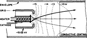
The diagram also shows the electron paths that originate at the emitting area of the cathode. It can be seen that those which leave the cathode at right angles cross the axis at a point not far from the cathode. This is a consequence of the powerful lens action of the strongly curved equipotential surfaces in the grid aperture. But, as electrons are emitted with random thermal velocities in all directions to the normal, the ‘cross-over’ is not a point but a small patch, the image of which appears on the screen when the spot is adjusted to maximum sharpness.
The conically shaped beam of divergent electrons from the electron gun have been accelerated as they rise up the steep potential gradient. The electrical potentials of the remaining nickel anodes, together with the post-deflection accelerating anode formed by the graphite coating, are selected to provide additional acceleration and, by field shaping, to refocus the beam to a spot on the screen. To achieve sharply defined traces it is essential that the focused spot should be as small as possible; the area of this image is, in part, dictated by the location and size of the ‘point source’ formed in front of the cathode. The rate at which electrons emerge from the cathode region is most directly controlled by adjustment of the negative potential of the grid; this is effected by the external brightness control. A secondary result of changes in the brightness control may be to modify, slightly, the shape of the point source. The slight de-focusing effect is corrected by the focus control, which adjusts an anode potential in the electron lens assembly.
11.8.1.2 Performance (electrostatic deflection)
If an electron with zero initial velocity rises through a potential difference V, acquiring a speed u, the change in its kinetic energy is ![]() , so that the speed is
, so that the speed is
using accepted values of electron charge, e, and rest-mass, m. The performance is dependent to a considerable extent on the beam velocity, u.
The deflection sensitivity of the tube is increased by shaping the deflection plates so that, at maximum deflection, the beam grazes their surface (Y1Y2; Figure 11.12). The sensitivity and performance limits may be assessed from the idealised diagrams (and notation) in Figure 11.14. Experience shows that a good cathode-ray tube produces a beam-current density Js at the centre of the luminous spot in rough agreement with that obtained on theoretical grounds by Langmuir, i.e.

where Jc is the current density at the cathode, V is the total accelerating voltage, T is the absolute temperature of the cathode emitting surface, θ is one-half of the beam convergence angle, and k is a constant. If ib is the beam current, then the apparent diameter of the spot is given approximately by ![]() .
.
The voltage Vd applied to the deflection plates produces an angular deflection δ given by
Deflection is possible, however, only up to a maximum angle α, such that
From these three expressions, certain quantities fundamental to the rating of a cathode-ray tube with electric field deflection can be derived.
11.8.1.3 Definition
This is the maximum sweep of the spot on the screen, D = 2αL, divided by the spot diameter, i.e. N = D/s. In television N is prescribed by the number of lines in the picture transmission. In oscillography N is between 200 and 300. Better definition can be obtained only at the expense of deflection sensitivity.
11.8.1.4 Specific deflection sensitivity
This is the inverse of the voltage that deflects the spot by a distance equal to its own diameter, i.e. the voltage which produces the smallest perceptible detail. The corresponding deflection angle is δ0 = s/L. Use of equations (11.1)–(11.3) gives for the specific deflection sensitivity
where k1 is a constant. Thus, the larger the tube dimensions the better the sensitivity at the smallest beam power consistent with adequate brightness of trace.
11.8.1.5 Maximum recording speed
The trace remains visible so long as its brightness exceeds a certain minimum. The brightness is proportional to the beam power density VJ, to the luminous efficiency σ of the screen, and to the time s/U during which the beam sweeps at speed U over one element of the screen. Hence,
Recording speeds up to 40 000km/s have been achieved with sealed-off tubes, permitting single-stroke photography of the trace.
11.8.1.6 Maximum specified recording speed
Unless compared with the spot size s, the value of U does not itself give adequate information. The specific speed Us= U/s is more useful: it is the inverse measure of the shortest time-interval in which detail can be recorded. Combining equations (11.5) and (11.1)
The product ζ(Vθ)2 is the essential figure in the speed rating of a cathode-ray tube.
11.8.1.7 Limiting frequency
A high recording speed is useful only if the test phenomena are recorded faithfully. The cathode-ray tube fails in this respect at frequencies such that the time of passage of an electron through the deflection field is more than about one-quarter of the period of an alternating quantity. This gives the condition of maximum frequency fm:
which means that the smallest tube at the highest acceleration voltage has the highest frequency limit. This conflicts with the condition for deflection sensitivity. Combining the two expressions gives the product of the two:
Compromise must be made according to the specific requirement. It may be observed that the optimum current ib is not zero as might appear, because for such a condition the convergence angle θ is also zero. In general, the most advantageous current will not differ from that for which the electron beam just fills the aperture.
Limitation of cathode-ray-tube performance by space charge is an effect important only at low accelerating voltages and relatively large beam currents. For these conditions the expressions above do not give practical ratings.
11.8.1.8 Fluorescent screen
The kinetic energy of each incident electron is converted into light owing to the exchange of energy which occurs within the phosphors coated on the inside of the screen. The result, luminescence, is usually described as either fluorescence or phosphorescence. Fluorescence is the almost instantaneous energy conversion into light, whereas phosphorescence is restricted to the phosphors which ‘store’ the converted energy and release it, as light, after a short delay. The afterglow can last many seconds. The respective terms are applied to the phosphors in accordance with their dominant light-emitting behaviour; however, each property is always present in a phosphor. In most cathode-ray tubes fluorescent phosphors are used with a very short afterglow (40 μs); a longer afterglow would blur a quickly changing display.
The most common fluorescent substances are silicates and sulphides, with calcium tungstate for photographic work. An excellent zinc silicate occurs naturally in the mineral willemite, but all other substances are prepared artificially. After purification, the substances are activated by the addition of very small quantities of suitable metals, and then ground to a powder of grain size 5–10 μm (for sulphides 10–50 μm).
In applying the powder to the glass several methods are used. Very finely ground silicates can be applied without a binder, by setting the powder from water, or an electrolyte. Sulphides are usually compounded with the glass wall by means of a binder such as sodium silicate; good results have been obtained also by baking them directly into the glass. In choosing the method two conflicting considerations must be taken into account. Baking or compounding gives good thermal contact, and prevents overheating of the powder particles by the electron beam. But at the same time good optical contact is established with the glass, with the result that light from the powder enters the glass also at angles exceeding the total reflection angle. This part of the light cannot escape at the viewing side, but is reflected and forms a luminous ‘halo’ which blurs the picture.
While silicates fluoresce usually green or blue-green, white fluorescence can be obtained by mixing cadmium sulphide and zinc cadmium sulphide in suitable proportions. The luminous efficiency of modern fluorescent powders is very high. Zinc silicate emits up to 2.5cd/W of beam power, and some sulphides are even more effective. The luminous efficacy increases with voltage up to about 10 kV, beyond which it decreases, partly because fast electrons are not stopped by the crystal grains.
The range of phosphors is classified by ‘P’ numbers, as in Table 11.4.

The light persistence of the most widely used phosphor (P31) is 40 μs; however, there are tubes available, using this phosphor, which have both variable persistence and ‘mesh storage’ facilities. Adjustable persistence enables very-low-frequency signals, lasting for a minute, to be viewed as a complete trace while retaining the normal ‘writing’ properties of the tube. Storage, at reduced brightness, is possible for up to 8 h.
Phosphor materials are insulators. The current circuit for all the incident beam electrons is completed by an equal number of low-energy electrons being attracted along various paths through the vacuum to the positive conducting-graphite coating. The result of secondary emission of electrons is to leave the screen with a positive charge only a little lower in potential than that of the graphite coating; thus, the surplus secondary emission electrons return to the phosphor-coated screen surface. This mechanism works perfectly at the voltages usually employed in oscillography and television (3–20 kV), also in small projection-tube sealed-off high-speed oscillographs (10–25 kV). Above 25 kV the mechanism is unsatisfactory and the dispersion of charge has to be supplemented by other means.
The power concentration in the luminous spot of a cathode-ray tube is very high. In direct-vision television tubes the momentary luminance may exceed 10 cd/mm2. A 3 mA 80 kV beam of a large-screen projection tube may be concentrated in an area of 0.1 mm2, representing a power density of 2kW/mm2. (By comparison, melting tungsten radiates about 10 W/mm2.) The width of the trace in a conventional 10 kV cathode-ray tube with a beam current of 10 μA is only 0.35 mm.
11.8.2 Deflection amplifiers (analogue c.r.o.)
Amplifiers are built into cathode-ray oscilloscope (c.r.o.) equipment to provide for time base generation and the amplification of small signals. The signals applied to the vertical (Y) deflecting plates are often repetitive time functions. To display them on a time base, the vertical displacements must be moved horizontally across the screen at uniform speed repeatedly at intervals related to the signal frequency, and adjusted to coincidence by means of a synchronising signal fed to the time base from the Y amplifier.
An additional constraint may be the requirement to start the time base from the left side of the screen at the instant the Y-plate signal is zero: a synchronising trigger signal is fed to the time base circuit to initiate each sweep. Finally, the spot must return (flyback) to the origin at the end of each sweep time. Ideally, flyback should be instantaneous: in practice it takes a few score nanoseconds. During flyback the beam is normally cut off to avoid return-trace effects, and this is the practice for television tubes.
Linear time bases are described in terms either of the sweep time per centimetre measured on the horizontal centre line of the graticule, or of the frequency. The repetition frequency range is from about 0.2 Hz to 2.5 MHz.
11.8.2.1 Ramp voltage (saw-tooth) generator
If a constant current I is fed to a capacitor C, its terminal voltage increases linearly with time. An amplified version of the voltage is applied to the X plates. Various sweep times are obtained by selecting different capacitors or other constant current values.
The method shown in Figure 11.15 employs a d.c. amplifier of high gain −G with a very large negative feedback coupled through an ideal capacitor Cf. The amplifier behaves in a manner dictated by the feedback signal to node B rather than by the small direct input voltage Es. The resultant signal vi is small enough for node B to be considered as virtually at earth potential. Analysing the network based on the ‘virtual earth’ principle, then v1 = 0 and ii = 0, the input resistance Ri being typically 1 MΩ. Then is + if = 0, whence

The output voltage vo increases linearly with time to provide the ramp function input to the X amplifier.
11.8.2.2 Variable delay
When two similar X amplifiers, A and B, are provided, B can be triggered by A; if B is set for, say, five times the frequency of A and this had a variable delay facility, then any one-fifth of the complete A waveform display can be extended to fill the screen. Both complete and expanded waveforms can be viewed simultaneously by automatic switching of A and B to the X plates during alternate sweeps.
11.8.2.3 Signal amplifiers
The X- and Y-plate voltages for maximum deflection in a modern 10 cm cathode-ray tube may lie between 30 and 200 V. As many voltage phenomena of interest have amplitudes ranging between 500 V and a few millivolts, both impedance matched attenuators and voltage amplifiers are called for. The amplifiers must be linear and should not introduce phase distortion in the working frequency range; the pulse response must be fast (e.g. 2 ns); and the drift and noise must be small (e.g. 3 μV).
Amplifiers have d.c. and a.c. inputs. The d.c. coupling is conventional, to minimise the use of capacitors (which tend to produce low-frequency phase distortion). The d.c. inputs also permit the use of a reference line. The a.c. input switch introduces a decoupling capacitor.
Two separate Y amplifiers are often provided; in conjunction either with one switched or with two separate X amplifiers, they permit the examination of two voltages simultaneously. It is important to distinguish the dual-trace oscilloscope (in which a single beam is shared by separate signal amplifiers) and the true double-beam device (with a gun producing two distinct beams).
11.8.3 Instrument selection
A general purpose c.r.o. must compromise between a wide frequency range and a high amplification sensitivity, because high gain is associated with restricted bandwidth. An economically priced c.r.o. with solid state circuitry may have a deflection sensitivity of 5 mV/cm, bandwidth 10 MHz and a 3 kV accelerating voltage for a 10 cm useful display. For greater flexibility, many modern c.r.o.s comprise a basic frame unit with plug-in amplifiers; the frame carries the tube, all necessary power outlets and basic controls; the plug-in units may have linear or special characteristics. The tube must be a high-performance unit compatible with any plug-in unit. The cost may be higher than that of a single function c.r.o., but it may nevertheless be economically advantageous. Many classes of measurement are catered for by specially designed oscilloscopes. In the following list, the main characteristic is given first, followed by the maximum frequency, deflection sensitivity and accelerating voltage, with general application notes thereafter.
Low-frequency (30 MHz, or 2 MHz at high gain; 0.1 mV/cm–10 V/cm; 3–10 kV). General purpose oscillography, for low-frequency system applications. Usually, high X-sweep speeds are needed for transient displays and complex transducer signals. Two traces available with two-beam or chopped single-beam tube. Single-shot facility. Y-amplifier signal delay useful for ‘leading-edge’ display. Rise times 10–30 ns.
Medium-frequency (100 MHz; 0.1 mV/cm; 8–15 kV). General-purpose, including wide-band precision types with a rise time of 3–10 ns.
High-frequency (non-sampling) (275 MHz; 10 mV/cm; 20 kV). May include helical transmission-line deflecting plates. Rise time 1.5 ns for testing digital system and computer displays.
Variable persistence storage cathode-ray tube for h.f. transients.
Very-high frequency (sampling) (12000 MHz; 5 mV/cm; 20 kV). The v.h.f. waveforms are ‘instantaneously’ measured and optically stored, n times at n successively retarded instants during the period of each of n successive waveforms (with n typically 1000). The n spots accumulate in the correct time sequence as a single waveform derived from the n waveforms sampled.
Large-screen (20 MHz; 60 mV/cm; 28 kV). Screen area up to 0.25 m2. Useful for industrial monitoring, classroom display and computer graphics. (Magnetic deflection gives a shorter overall length of tube, probably with improved focusing towards the edges but with a lower maximum frequency.)
11.8.3.1 Other features
With all c.r.o.s, the X–Y cartesian coordinate display can be augmented by Z-modulation. This superimposes a beam-intensity control on the X–Y signals to produce the illusion of three dimensions. The beam control may brighten one spot only, or gradually ‘shape’ the picture.
Oscilloscopes are supplemented by such accessories as special probes for matching and/or attenuating the signal to the signal/cable interface. Anti-microphony cables are available which minimise cable-generated noise and capacitance change. Many types of high-speed camera can be used, including single-shot cameras that can employ ultraviolet techniques to ‘brighten’ a record from a trace of low visual intensity.
11.8.4 Operational use
To avoid degradation of the signal source, a c.r.o. has a high input impedance (1 MΩ, 20 pF) and a good common-mode rejection (50 dB). The quality can be considerably impaired by impedance mismatch and incorrect signal/earth (or ground) connections.
11.8.4.1 Impedance matching
Voltage signals are often presented to a c.r.o. through wires or coaxial cables terminated on crocodile clips. Although this may be adequate at low frequencies, it can behave like a badly matched transmission line, causing attenuation distortion and phase distortion. The earth screen of a coaxial cable is not fully effective, and in consequence the cable can pick up local radiated interference. In a normal cable the central conductor is not bonded to the insulation, and flexure of the cable may distort the signal waveform because of changes in the capacitance distribution, or generated noise. The cable capacitance of about 50 pF/m is additive to the c.r.o. input capacitance, and will distort the signal, particularly if the frequency and source impedance are high.
These adverse effects can be mitigated by use of fully screened probes and cables of low and constant capacitance associated with low loss. The probes may be active (including an impedance matching unity-gain amplifier) or passive (including resistance with adjustable capacitance compensation); attenuators are incorporated in each to reduce both the signal level and the capacitive loading of the source, the compensation being most effective for high-impedance sources. The active probe can be used to match the source to the standard 50Ω input impedance of a high-frequency c.r.o. (100 MHz and above), an important matter in that a quarter wavelength at 100 MHz is about 75 cm, and severe standing-wave effects may otherwise occur to invalidate the measurements.
11.8.4.2 Earths and grounds
Ground planes (e.g. extended screens) and earth planes (e.g. trunking) constitute low-impedance paths through which interfering signals can circulate, of a wide variety of frequencies and waveforms. The arbitrary connection of screens to earth and ground terminals can have the unwelcome result of increasing noise, due to earth-loop currents. The latter must not enter the input signal lines of either the system or the c.r.o.; and the interference can be minimised by using a single ground/earth connection to serve the whole equipment, if this is possible. The common connection should be made at the zero-potential input signal lead.
11.8.5 Calibration
Operational specifications will include performance statements, typically: voltage accuracy, ±3%; time-base frequency ±3%; Y-amplifier linearity, ±3%, phase shift, 1°; pulse response, ![]() 5% after 2 ns; sweep delay accuracy, ±2%. The calibration facility provided usually consists of a 1 or 2 kHz square waveform with a 3 us rise time, with both the frequency and voltage amplitude within ±1%.
5% after 2 ns; sweep delay accuracy, ±2%. The calibration facility provided usually consists of a 1 or 2 kHz square waveform with a 3 us rise time, with both the frequency and voltage amplitude within ±1%.
The practical application of the c.r.o. as a test instrument includes (a) the general diagnostic display of waveforms, and (b) the testing of a product during development or manufacture in relation to its accuracy and quality control. For (a) the built-in calibration facility is adequate; but for (b) it is prudent (or essential) to make regular checks of the actual parameters of the self-calibration facility and of the basic characteristics of the instrument. Such tests would include assessments of the accuracy on alternating voltages, and the ratio and phase angle of the amplifiers and attenuators over the frequency range. The most important and critical test for a c.r.o., which will inevitably be used with modern digital networks, is its response to high frequency square waveforms. The rise time is quite easily measured, but the initial resonant frequency of the ‘flat’ part of the waveform and its rate of attenuation are important in assessing the actual duration of this part.
The quality and usefulness of these tests is ultimately related to the readability of the display, which would be no better than ±0.3% in a 10 cm trace. The quality of the standard reference devices would, for example, be ±0.1% for a variable-frequency alternating voltage source; hence, there would be a total measurement uncertainty of about 0.4% in the ±1% waveform. It follows that the actual c.r.o. voltage source must be correct to within 0.6% if it is to be used with confidence as a ±1% source. It is a fundamental requirement that the quality of all the reference standards be known from recent linearity and traceability tests.
11.8.6 Applications
The principal application is for diagnostic testing. In addition, the c.r.o. is used to monitor the transfer characteristics of devices and systems, as well as for numerical measurements. Among special uses are to be found the television camera, electron diffraction camera and electron microscope.
Single-deflection measurements The tube functions with a single pair of deflecting plates as a voltmeter or ammeter, with the advantages of being free from damping, unaffected by change of frequency or temperature or over-deflection, and imposing only a minute load on the test circuit. Examples are the monitoring of signals in broadcast and recording studios, modulation checks, indication of motor peak starting currents, thickness measurement, null detection and the measurement of current and voltage in networks of very low power.
Differential measurements: Similar or related phenomena are compared by use of both pairs of deflecting plates, the resulting Lissajous figure being observed. In this way phase difference can be measured, frequencies accurately checked against a standard, armature windings tested, modulation indicated by a stationary waveform, and the distortion measured in receivers, amplifiers and electro-acoustic equipment. Figure 11.16 is a Lissajous figure comparing two frequencies by counting the horizontal and vertical loops, giving the ratio 4/5. The diagram in Figure 11.17 shows the connections for testing the distortion of an amplifier: the oscillator is set to a known frequency, the two pairs of deflectors connected, respectively, to the input and output (with suitable attenuators). A straightline display indicates absence of distortion, while curvature or looping indicates distortion.


Repetitive time base: Using a linear time base enables sustained waveforms to be displayed for machines, transformers and rectifiers, rapid operations to be timed, and surge phenomena to be shown with the aid of a recurrent-surge generator.
Single sweep: Non-repetitive transients, such as those arising by lightning or switching, are most readily traced by use of the continuously evacuated tube, but sensitive sealed-off tubes can also be employed. In either case a non-repetitive time base is used consisting of the voltage of a capacitor discharged through a resistor and triggered by a gap. The transient discharge is normally obtained by use of a surge generator for power system plant testing, but other single transients, such as the small voltages of cardiac origin, may also require to be recorded.
Independent bases: The c.r.o. is well suited to the display of quantities related by some variable other than time. The current due to an impressed voltage can be displayed on a frequency base as a resonance curve, radio receivers aligned, and B/H loops taken for steel samples. Transistor curve tracers are useful applications capable of giving a complete family of characteristics in a single display.
Modified time bases: There are several modified forms of time base. If two voltages of the same amplitude and frequency are displaced in time phase by a quarter-period and applied, respectively, to the X and Y plates as in Figure 11.18, they will produce a circular trace. One application, in decade digital logic circuits, involves a Z modulation of the c.r.o. grid. To check that a frequency divider section is working correctly, the period of the circular time base is made 10 times that of the next higher count rate section. With the latter used to modulate, 10 equal bright and dark peripheral sectors should appear on the trace.

11.8.7 Digital storage oscilloscopes
Digital storage oscilloscopes (d.s.o.) (Figure 11.19) offer advantages over the analogue c.r.o. in some circumstances:

(1) they allow long-term display of a transient quantity;
(2) it is easy to produce a hard copy of the display;
(3) they allow computation and signal processing within the d.s.o.;
(4) they allow easy transfer of data to a computer; and
(5) they use cheap cathode-ray-tube construction because the deflection is not at signal frequency but much lower than the maximum signal frequency.
The d.s.o. has become available for laboratory and industrial use because of the development of relatively cheap, accurate and fast A/D converters.
11.8.8 Digital oscilloscope characteristics
Clearly the sampling rate must be high enough to give a faithful representation of the applied signal. Nyquist’s theorem states that a periodic signal must be sampled at more than twice the highest frequency component of the signal. In practice, because of the finite time available, a sample rate somewhat higher than this is necessary. A sample rate of 4 per cycle at oscilloscope bandwidth would be typical. Therefore, for single shot, a digital oscilloscope specification will give a bandwidth of 100 MHz or a sample rate of 400 megasamples/s. If the display is a dot display, then something like 20 samples per cycle is necessary if the eye is to interpret the display easily. Usually some form of interpolation is provided to aid interpretation. The simplest method is to draw straight lines between successive sample parts. Other interpolation methods are used such as sine interpolation, designed for fairly pure sine waves. This interpolation will give erroneous displays for non-sinusoidal inputs.
All this means that great care must be taken in interpreting a display when the input approaches the oscilloscope bandwidth, particularly if it has significant high frequency components such as a square wave. This is also true of course for an analogue c.r.o.
The d.s.o. in repetitive mode can build up the display over a number of sections of the displayed waveform, and so the sampling-rate problems are not so severe. Specifications will give bandwidth, single-shot bandwidth and sampling rate. If single-shot mode is to be used, then care must be taken to look for the adequacy of the single-shot bandwidth or the sampling rate.
For an analogue c.r.o., a rule of thumb relates the rise time of the c.r.o. to its bandwidth rise time (s) × bandwidth (Hz) = 0.35. So, a 100 MHz oscilloscope has a rise time of 3.5 ns. A signal rise time approaching this cannot be faithfully displayed, as the fastest displayed rise time is that of the instrument itself. Usually the fastest rise time display-able is 8 times the c.r.o. rise time. So the fastest signal rise time = 2.8 ÷ bandwidth. For a 100 MHz c.r.o. this would be 28 ns.
A similar restriction occurs for the d.s.o. A fast signal pulse on an expanded time scale is shown in Figure 11.20. The worst case giving the slowest rise time is when one of the samples is in the middle of the edge. The time from 10% to 90% of the rise (the rise time) is given by (80/100) × 2 sample periods (= 1.6 sample periods).

So for a 100 megasample/s d.s.o., the sampling interval is 10 ns and the displayed edge, regardless of the rise time of the applied signal, is at worst 16 ns. Again, in order to faithfully display the signal, and not the characteristics of the d.s.o., the fastest signal rise time should be about 8 times this limit, say 10 sample intervals. So, as a rule of thumb:

e.g. for 100 megasamples/s d.s.o. the fastest signal rise time is 100 ns. For a signal rise time faster than this it is likely that the performance of the d.s.o. will show itself in the display of the signal.
11.8.8.2 Vertical resolution
Vertical resolution is another important parameter of the d.s.o. An important contribution to this is the number of bits of the A/D converter. The more bits, the greater the resolution. The minimum discernible level is
where n is the number of bits of the A/D.
For example, for an input voltage of 1 V and an 8-bit A/D, the minimum discernible level is
This value is sometimes given as a percentage and in this case would be ±0.2%.
So on a 1-V signal, noise of less than 4 mV will not be displayed. Increasing the number of bits in the A/D converter will help, but internally generated noise limits the advantage achieved. This leads to the concept of effective bits of the d.s.o., which is performance of a hypothetical idealised A/D converter which gives the same vertical resolution of the actual A/D converter with its noise limitation.