
22
MARGINAL RATE OF TRANSFORMATION AND RATE OF SUBSTITUTION
22.1 INTRODUCTION
This chapter1 discusses the use of DEA environmental assessment to measure the marginal rate of transformation (MRT) and rate of substitution (RSU) among production factors, in particular between desirable and undesirable outputs. In the methodological concern, this chapter is an extension of Chapter 9 which discusses the quantitative approach on MRT within a conventional framework of DEA. In discussing the new approach for measuring MRT and RSU, it is necessary for us to describe that both estimates depend upon the magnitude and sign of dual variables, or multipliers, obtained from the proposed formulations. A problem associated with the estimation of MRT and RSU is that the two measures often become unstable, so often being inconsistent with economic and/or business reality, because DEA does not assume any functional form among the three production factors (X, G and B). The non‐parametric feature makes the DEA‐based MRT and RSU measurement very difficult because it often produces large or small multipliers. As a result, DEA does not attain a high level of estimation accuracy and thus has limited practicality. Consequently, almost no previous studies have explored the measurement of MRT and RSU, only paying attention to efficiency measurement. Exceptions can be found in Cooper et al. (2000)2 and Asmild et al. (2006)3.
To overcome such a research difficulty, the proposed measurement of MRT and RSU pays attention to two research concerns. One of the two concerns is how to restrict dual variables in such a manner that computational results are consistent with our expectation and prior information. Conventional approaches are often referred to as “multiplier restriction” methods. For example, Charnes et al (1989)4 and Thompson et al. (1990)5 provided their descriptions on “CR: cone ratio approach” and “AR: assurance region analysis,” respectively, which have long served as well‐known multiplier restriction methods. See Chapter 4 on the multiplier restriction methods. This chapter extends the multiplier restriction to environmental assessment by proposing “explorative analysis.” An important feature of the proposed approach is that it can avoid prior information on multiplier restriction. It can be easily imagined that we have a difficulty in accessing prior information for restricting multipliers. The proposed explorative analysis can overcome such a difficulty related to the multiplier restriction.The other important research concern is that this chapter incorporates the concept of desirable congestion (DC), discussed in Chapter 21, into the measurement of MRT and RSU. This chapter considers that an occurrence of DC is more important than undesirable congestion (UC) because the former occurrence indicates eco‐technology innovation. As mentioned previously, the underlying philosophy of this book is that we are interested in policy and business concerns for reducing the global warming and climate change by eco‐technology innovation (e.g., clean coal technology in the electricity industry and hybrid cars in the automobile industry) along with related managerial challenges (e.g., a fuel mix strategy from coal to natural gas and other renewable energies in the electricity industry).
This chapter acknowledges that the research of Cooper et al. (2000) was the first to provide DEA‐based MRT and RSU in the framework of inputs and desirable outputs. Acknowledging their contribution, however, this chapter needs to mention that they have never considered an output separation into desirable and undesirable categories. Consequently, it is impossible for us to incorporate their approach on MRT and RSU into the environmental assessment proposed in this chapter.
The remainder of this chapter is organized as follows: Section 22.2 discusses economic and strategic concepts used in this chapter. Section 22.3 briefly discusses the possible occurrence of DC, as an extension of Chapter 21, and extends it to the measurement of MRT and RSU. Section 22.4 discusses the analytical structure of MRT and RSU. Section 22.5 describes multiplier restriction for the two measures. Section 22.6 discusses the explorative analysis, incorporated into the proposed environmental assessment. Section 22.7 applies the proposed approach to nations in Europe and North America. Section 22.8 summarizes this chapter.
22.2 CONCEPTS
22.2.1 Desirable Congestion
Returning to Figure 15.6 in Chapter 15, Figure 22.1 depicts the unification process between desirable and undesirable outputs. Since Chapter 15 provides a description on the top of Figure 22.1, this chapter starts with the middle of Figure 22.1, which describes an occurrence of DC in the g–b space, where g and b indicate desirable and undesirable outputs in horizontal and vertical coordinates, respectively. To simplify our visual description, we consider a case of a single component of the three vectors for production factors (i.e., X, G and B).
FIGURE 22.1 Damages to return under managerial disposability (a) The middle of the figure assumes that an undesirable output (b) is a byproduct of a desirable output (g). (b) The type of DTR is classified into decreasing, constant and increasing under no DC. See Chapter 23 for a description of DTR.
Here, in shifting our description from the top to the middle and bottom of Figure 22.1, we need to consider that “undesirable outputs are byproducts of desirable outputs.” In the middle and bottom of the figure, the negative slope of the supporting hyperplane indicates the occurrence of strong DC, or eco‐technology innovation for reducing the undesirable output (i.e., industrial pollution). In contrast, a positive slope implies the opposite case (i.e., no occurrence of DC), so there is no DC. An occurrence of weak DC is identified between strong and no DC, so being weak DC.
The bottom of Figure 22.1 depicts the three types of DC: no, weak and strong DC in the g–b space. Under the occurrence of no DC, damages to return (DTR) is separated into three categories: constant, increasing and decreasing. An occurrence of eco‐technology innovation under managerial disposability is identified by negative DTR, or strong DC, in the case where three production factors have a single component. When the three production factors have multiple components, the occurrence of strong DC becomes a necessary condition of negative DTR, but not sufficient. See Chapter 23 on the classification of DTR.
22.2.2 MRT and RSU
Figure 22.2 depicts RSU among an input (x), a desirable output (g) and an undesirable output (b). As depicted in Figure 22.2, for example, dg/dx measures the degree of MRT where d stands for the derivative on a functional form between g and x. In a similar manner, the degree of MRT is applicable to other relationships among x, g and b. It can be intuitively considered that the MRT measures the rate at which a DMU willingly exchanges an amount of a production factor for another one.

FIGURE 22.2 Marginal rate of transformation and rate of substitution
The degree of (dg/dx)/(g/x) measures a magnitude of RSU that is considered as “scale elasticity” when the two vectors (X and G) have a single component. The analytical relationship is applicable to the other two cases (b and x; g and b) in the manner of (db/dx)/(b/x) and (db/dg)/(b/g).
Here, it is important to note that RSU, explored in this chapter, is different from elasticity of substitution (ES) that serves as a fundamental concept of economics. Both measures have similarities and differences in many aspects. To describe the position of RSU more clearly, this chapter reviews ES and then compares it with RSU.
Elasticity of Substitution (ES):
The concept of ES has a long history in economics, dating back to the original concept proposed by Hicks (1932)6. He used ES as a methodology for analyzing between capital and labor income shares in a growing economy, along with constant RTS and a natural technology change. Allen and Hicks (1934)7 and Allen (1938)8 extended the original concept of ES. Uzawa (1962)9 further analyzed the concept, becoming a dominant concept of ES, conventionally referred to as “Allen–Uzawa elasticity” in modern economics. Later, Morishima (1967)10 proposed an alternative to the Allen–Uzawa elasticity, referred to as “Morishima elasticity,” to which many economists (Davis and Gauger, 1996; Klump and de la Grandville, 2000) 11,12 paid attention because it fitted with various functional forms to represent production and/or cost functions.
It is indeed true that such previous works in economics made a major contribution on the ES measurement. However, this chapter needs to mention the following five concerns on how the proposed RSU is different from the conventional ES in environmental assessment.
First, all the previous studies assumed a flexible functional form, or so‐called “distance function,” to express a production function or a cost function. However, none knows what the most appropriate functional form is in reality. A methodological contribution of DEA is that it can avoid a specification error of such a distance function.
Second, another assumption associated with ES was that a functional form used for measuring the degree should be twice differentiable because both Allen–Uzawa and Morishima ES measures needed to take a derivative on a distance function that was usually a quadratic functional form. For example, Hicks (1932, pp. 241–246) proposed the following ES between two inputs:
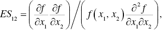
where the symbol (f) stands for a functional form as well as x1 and x2 indicate the amount of inputs, respectively. The symbol (![]() ) indicates a partial derivative of a functional form. All the proceeding studies in economics followed the above definition on ES along with their extensions. Acknowledging the importance of the original definition on ES and its extension (e.g., Morishima, 1967), this chapter does not follow that definition of ES, rather measuring the derivative of a distance function by dual variables, or multipliers, of linear programming because this chapter is concerned with the measurement of RSU, so not conventional ES, within the framework of DEA environmental assessment.
) indicates a partial derivative of a functional form. All the proceeding studies in economics followed the above definition on ES along with their extensions. Acknowledging the importance of the original definition on ES and its extension (e.g., Morishima, 1967), this chapter does not follow that definition of ES, rather measuring the derivative of a distance function by dual variables, or multipliers, of linear programming because this chapter is concerned with the measurement of RSU, so not conventional ES, within the framework of DEA environmental assessment.
Third, previous studies in economics assumed that all entities in private and public sectors worked efficiently without any loss or any inefficiency. Consequently, the previous studies could measure their ES measures on an efficiency frontier, or on the surface of a distance function to represent the efficiency frontier. That was for mathematical convenience. The reality is much different from the economic assumption. In contrast, DEA can measure the degree of efficiency or inefficiency without the assumption. Thus, the DEA‐based RSU measurement becomes conceptually more practical than the ES measurement in economics. However, nobody knows which is accurate or not in reality because all methodologies are approximations.
Fourth, previous studies in economics often imposed many assumptions such as linear homogeneity and symmetry on input prices on a functional form. In contrast, DEA can avoid such economic assumptions for specifying a functional form. Thus, DEA has more practicality than the conventional approaches proposed in economics.
Finally, Sueyoshi and Goto (2012d) discussed how to measure MRT and RSU within the computational framework of DEA environmental assessment. Their study did not measure the degree of these scale‐related measures. The measurement is important because when we examine a large production process, as found in energy sectors, the environmental assessment needs to consider these scale‐related measures. Furthermore, their estimates may become unstable because an efficiency frontier, measured by DEA, consists of a piece‐wise linear polyhedron surface, so not assuming any functional form. Therefore, the multiplier (dual variable) restriction method is necessary for obtaining reliable MRT and RSU estimates on the frontier. The methodological issue will be discussed in this chapter, hereafter.
22.3 A POSSIBLE OCCURRENCE OF DESIRABLE COnGESTION (DC)
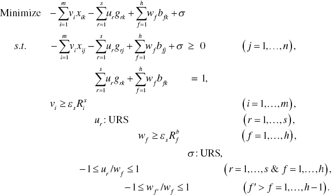
As depicted in Figure 22.1, this chapter incorporates a possible occurrence of DC into the proposed environmental assessment under managerial disposability because we are interested in eco‐technology innovation for pollution reduction. To examine the occurrence, this chapter starts with the following model (22.2) for our descriptive convenience:
The model has the following dual formulation:
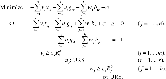
As discussed in Chapter 21, an important feature of Model (22.3) is that the dual variables (ur: URS for r = 1,…, s) are unrestricted in these signs because Model (22.2) does not have slacks related to desirable outputs (G).
A unified efficiency measure, or ![]() , of the k‐th DMU under managerial disposability becomes as follows:
, of the k‐th DMU under managerial disposability becomes as follows:
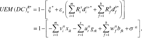
where all variables are determined on the optimality of Models (22.2) and (22.3). The equation within the parenthesis, obtained from the optimality of Models (22.2) and (22.3), indicates the level of unified inefficiency under managerial disposability. The unified efficiency is obtained by subtracting the level of inefficiency from unity.
As discussed in Chapter 21, we solve Model (22.3) and then identify a possible occurrence of DC, or eco‐technology innovation, by the following rule along with the assumption on a unique optimal solution:
- If
 for some (at least one) r, then “weak DC” occurs on the k‐th DMU,
 - If
 for some (at least one) r, then “strong DC” occurs on the k‐th DMU and
 - If
 for all r, then “no DC” occurs on the k‐th DMU.
If ![]() for some r and
for some r and ![]() for the other r′, then the occurrence of weak and strong DCs coexist on the k‐th DMU. This chapter considers it as strong DC, so indicating eco‐technology innovation on undesirable outputs. It is important to note that
for the other r′, then the occurrence of weak and strong DCs coexist on the k‐th DMU. This chapter considers it as strong DC, so indicating eco‐technology innovation on undesirable outputs. It is important to note that ![]() for all r is the best case because an increase in any desirable output always decreases the amount of undesirable outputs. Meanwhile, if
for all r is the best case because an increase in any desirable output always decreases the amount of undesirable outputs. Meanwhile, if ![]() is identified for some r, then it indicates that there is a chance to reduce the amount of undesirable output(s). Therefore, this chapter also considers this case as an occurrence of DC.
is identified for some r, then it indicates that there is a chance to reduce the amount of undesirable output(s). Therefore, this chapter also considers this case as an occurrence of DC.
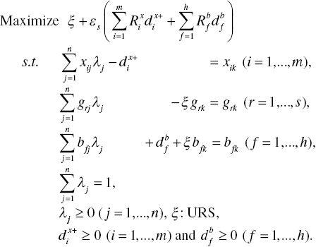
22.4 MEASUREMENT OF MRT AND RSU UNDER DC
In the case of a single component of the three production factors, this chapter estimates the degrees of MRT and RSU regarding the k‐th DMU under managerial disposability as follows:
Since the managerial disposability has a priority order in which environmental performance comes first and operational performance comes second, this chapter considers the MRT and RSU of b to the other two production factors (g and x). The superscript R stands for radial measurement.
For efficient DMUs:
This chapter can specify the degree of MRT and RSU of the k‐th DMU, having multiple components of the three production factors, which are measured under managerial disposability as follows:
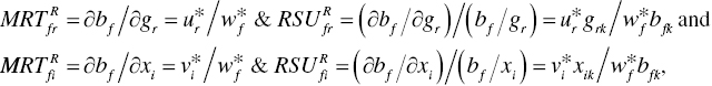
for all i = 1,…, m, r = 1,…, s and f = 1,…, h if the k‐th DMU is efficient. The dual variables are obtained from the optimality of Model (22.3).
For inefficient DMUs:
If the DMU is inefficient, the RSU measure needs to be adjusted as follows:
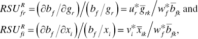
where the upper bar indicates the amount of each production factor on an efficiency frontier after adjusting the inefficiency score and slacks. The variables are adjusted by![]() (i = 1,..., m),
(i = 1,..., m), ![]() (r = 1,..., s) and
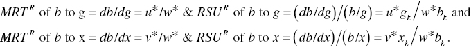
(r = 1,..., s) and![]() (f = 1,..., h),from the optimality of Model (22.2).Here, it is necessary for us to describe three analytical concerns on MRT and RSU. First, the determination of MRT and RSU needs to project an inefficient DMU onto an efficiency frontier by slack adjustment. See Chapter 9 on slack adjustment. However, it is expected in this chapter that the influence of slack adjustment on MRT and RSU may be less than that of multiplier restriction by the proposed explorative analysis. Therefore, this chapter does not utilize the adjustment, as discussed in Chapter 9. Second, Chapter 9 describes MRT of a desirable output (g) to an input (x). So, the MRT of the k‐th DMU becomes
(f = 1,..., h),from the optimality of Model (22.2).Here, it is necessary for us to describe three analytical concerns on MRT and RSU. First, the determination of MRT and RSU needs to project an inefficient DMU onto an efficiency frontier by slack adjustment. See Chapter 9 on slack adjustment. However, it is expected in this chapter that the influence of slack adjustment on MRT and RSU may be less than that of multiplier restriction by the proposed explorative analysis. Therefore, this chapter does not utilize the adjustment, as discussed in Chapter 9. Second, Chapter 9 describes MRT of a desirable output (g) to an input (x). So, the MRT of the k‐th DMU becomes ![]() . Meanwhile, the MRT of the k‐th DMU on the undesirable output b to x becomes
. Meanwhile, the MRT of the k‐th DMU on the undesirable output b to x becomes ![]() and the MRT of the k‐th DMU of b to g becomes
and the MRT of the k‐th DMU of b to g becomes ![]() . The difference can be found in the RSU measurement. See Figure 22.2. Finally, as discussed in Chapter 9, the degree of scale elasticity (for a single output) and the degree of scale economies (for multiple outputs) are defined on a projected point on an efficiency frontier. Since DEA environmental assessment has desirable and undesirable outputs, this chapter looks for the degree of scale economies. However, the degree of RSU measured by Equations (22.6) and (22.7) is related to a specific combination between two production factors. Therefore, the degree indicates “factor‐specific scale economy (elasticity).” Such indicates conceptual differences between Chapter 9 for DEA and this chapter for DEA environmental assessment.
. The difference can be found in the RSU measurement. See Figure 22.2. Finally, as discussed in Chapter 9, the degree of scale elasticity (for a single output) and the degree of scale economies (for multiple outputs) are defined on a projected point on an efficiency frontier. Since DEA environmental assessment has desirable and undesirable outputs, this chapter looks for the degree of scale economies. However, the degree of RSU measured by Equations (22.6) and (22.7) is related to a specific combination between two production factors. Therefore, the degree indicates “factor‐specific scale economy (elasticity).” Such indicates conceptual differences between Chapter 9 for DEA and this chapter for DEA environmental assessment.
22.5 MULTIPLIER RESTRICTION
In measuring MRT and RSU, it is possible for us to incorporate prior information as multiplier restrictions so that MRT and RSU estimates may belong to an acceptable range for a user. This chapter incorporates the following restrictions on multipliers (dual variables):
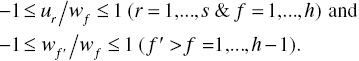
The first part of Equations (22.8) indicates multiplier restriction between the r'th desirable output and the f‐th undesirable output. The second part indicates the restriction between the f‐th and f′‐th undesirable outputs.
The proposed multiplier restriction has two analytical rationales. One rationale is that, as suggested in Chapter 2, this chapter divides each production factor by its average. Data manipulation is necessary for DEA to avoid the case where large data dominates small data in the computation. Otherwise, the computational result is often unreliable and misguiding. Thus, the data set on each production factor is unit‐less. The other rationale is that the data adjustment makes it possible for the resulting multiplier to indicate the importance of each production factor in the manner that each ratio locates between –100% and 100%, as formulated in Equations (22.8).
Model (22.3), incorporating Equations (22.8), becomes
In the history of DEA, the proposed multiplier restriction is often referred to as “assurance region (AR) analysis” and it has been used to reduce the number of efficient DMUs. See Chapter 4 for a description of AR analysis. That is indeed important because DEA usually produces many efficient DMUs. In contrast to the historical use, this chapter uses it for the measurement of MRT and RSU under managerial disposability. Furthermore, the proposed approach does not need any prior information on multiplier restriction, as required by AR analysis.
22.6 EXPLORATIVE ANALYSIS
Figure 22.3 visually describes Equation (22.8) as an “explorative analysis” which combines DEA‐based performance assessment with multiplier restriction to obtain acceptable empirical results. It is indeed true that the proposed explorative analysis originates from the AR analysis. However, there are two differences between the approach proposed in this chapter and the AR approach.
FIGURE 22.3 Explorative analysis (a) The proposed approach does not need prior information for multiplier restriction. The analytical feature is different from a conventional use of the AR analysis that needs prior information. See Chapter 4 on the AR analysis. (b) The explorative analysis implies that we investigate computational results by utilizing both a data set and additional information so that computational results can fit with our expectation and reality. (c) It is possible for us to change a combination on multiplier restriction for explorative analysis until we can satisfy MRT and RSU estimates in our expected ranges. Equations (22.8) can work most of data sets because each production factor is divided by each factor average. An exception is a data set with many zeros. In this case, we must depend on the methodologies listed in Chapters 26 and 27.
As depicted at the top of Figure 22.3, the proposed approach adjusts a data set in such a manner that each production factor is divided by the factor average. It is possible for us to apply a DEA environmental assessment, or Model (22.9), to the adjusted data set. A problem still exists in the manner that multipliers, or dual variables, become unstable in many cases. For example, they become very large and very small so that MRT and RSU estimates become very large or very small at these magnitudes. The result is often unacceptable. An approach to handle the difficulty with DEA is to restrict multipliers within an acceptable range that fits with our expectation. As discussed previously, the AR approach is one such multiplier restriction method. A problem of AR is that it needs prior information for multiplier restriction and as such is usually subjective. That is a drawback of the AR approach. In contrast, the exploration analysis does not use the prior information.
To overcome the subjectivity issue, the explorative analysis pays attention to a unique feature of the adjusted data set. That is, the data is unit‐less, because each production factor is divided by the factor average, so indicating the importance of each factor. The multiplier restriction, expressed by Equations (22.8), or ![]() and
and ![]() specifies the range of importance among desirable and undesirable outputs by a percentile expression between –1 and 1. Thus, the proposed approach can avoid our subjectivity on multiplier restriction. It is impossible for us to utilize the proposed explorative analysis without such a data adjustment at the initial stage of DEA environment assessment.
specifies the range of importance among desirable and undesirable outputs by a percentile expression between –1 and 1. Thus, the proposed approach can avoid our subjectivity on multiplier restriction. It is impossible for us to utilize the proposed explorative analysis without such a data adjustment at the initial stage of DEA environment assessment.
Finally, this chapter clearly understands that the proposed approach is one of many approaches for multiplier restriction. The approach may repeat several times until the computational result on MRT and RSU satisfies our expectation, as depicted in Figure 22.3.
22.7 INTERNATIONAL COMPARISON
Using Model (22.9), this chapter compares the performance of 25 industrial nations, all of which are members of Organization for Economic Co‐operation and Development (OECD). The data set used in this study is listed in the OECD library (http://www.oecd‐ilibrary.org/).
Data Accessibility:
the supplementary section of Sueyoshi and Yuan (2016a) provides a list of the whole data set used in this chapter.
The observed annual periods are from 2008 to 2012. All the nations are classified into the three reginal categories: Eastern European Union (EU), Western EU and North America. Eastern EU includes nations that were previously under socialism. Western EU consists of nations under capitalism13. North America contains Canada and the United States14. The EU nations are specified as follows: Eastern EU: Czech Republic, Estonia, Hungary, Poland, Slovak Republic, Slovenia and Western EU: Austria, Belgium, Denmark, Finland, France, Germany, Iceland, Ireland, Italy, Luxembourg, Netherlands, Norway, Portugal, Spain, Sweden, Switzerland, United Kingdom.
The data set used in this chapter consists of: (a) gross domestic product (GDP) as a single desirable output, (b) two undesirable outputs: particulate matter (PM) 2.5 and CO2 and (c) two inputs: the number of population and the total amount of energy supply. See Sueyoshi and Yuan (2016a) for a detailed description on the data set. Descriptive statistics can be found in their article.
Table 22.1 documents the computational results obtained by the model in Equation (22.9) for 2012. For example, the degree of ![]() regarding Austria was 0.726 in 2012. Here,
regarding Austria was 0.726 in 2012. Here, ![]() stands for unified efficiency under managerial disposability and with a possible occurrence of DC. See the first row of the table. Some countries exhibit a high level of efficiency (close to unity) in
stands for unified efficiency under managerial disposability and with a possible occurrence of DC. See the first row of the table. Some countries exhibit a high level of efficiency (close to unity) in ![]() , such as France, Germany, Hungary, Iceland, Italy, Luxembourg, Portugal, Spain, Sweden, Switzerland, United Kingdom and United States. This indicates that these countries have developed balanced economy and environment efficiency, so attaining the status of social sustainability.
, such as France, Germany, Hungary, Iceland, Italy, Luxembourg, Portugal, Spain, Sweden, Switzerland, United Kingdom and United States. This indicates that these countries have developed balanced economy and environment efficiency, so attaining the status of social sustainability.
TABLE 22.1 Computational results for 2012: Model (21.9).
(a) Source: Sueyoshi and Yuan (2016a). (b) ![]() indicates unified efficiency under managerial disposability with a possible occurrence of DC. (c) u/w1 is MRT of PM 2.5 (w1) to GDP (u). u/w2 is MRT of CO2 (w2) to GDP (u). w1/w2 is MRT of CO2 (w2) to PM 2.5 (w1). ug/w1b1 is RSU of PM 2.5 to GDP and ug/w2b2 is RSU of CO2 to GDP.
indicates unified efficiency under managerial disposability with a possible occurrence of DC. (c) u/w1 is MRT of PM 2.5 (w1) to GDP (u). u/w2 is MRT of CO2 (w2) to GDP (u). w1/w2 is MRT of CO2 (w2) to PM 2.5 (w1). ug/w1b1 is RSU of PM 2.5 to GDP and ug/w2b2 is RSU of CO2 to GDP.
| Country | ||||||
| Austria | 0.726 | 0.077 | 0.077 | 1.000 | 2.198 | 0.812 |
| Belgium | 0.779 | 0.116 | 0.116 | 1.000 | 1.552 | 0.661 |
| Canada | 0.674 | 1.000 | 0.000 | 0.000 | 1.258 | 0.000 |
| Czech Republic | 0.647 | –0.057 | –0.057 | 1.000 | –0.564 | –0.137 |
| Denmark | 0.720 | 1.000 | 0.014 | 0.014 | 23.924 | 0.245 |
| Estonia | 0.459 | –1.000 | 0.000 | 0.000 | –38.655 | 0.000 |
| Finland | 0.640 | 1.000 | 0.020 | 0.020 | 20.603 | 0.310 |
| France | 1.000 | –0.981 | –0.946 | 0.965 | –1.393 | 0.909 |
| Germany | 1.000 | –0.887 | –0.859 | 0.968 | –2.326 | 0.468 |
| Hungary | 1.000 | –0.918 | –0.263 | 0.287 | –4.701 | 1.302 |
| Iceland | 1.000 | –0.005 | –0.001 | 0.165 | –3.233 | 18.723 |
| Ireland | 0.707 | 0.020 | 0.020 | 1.000 | 1.399 | 0.393 |
| Italy | 1.000 | –0.980 | –0.843 | 0.860 | –1.883 | 0.731 |
| Luxembourg | 1.000 | 0.029 | 0.024 | 0.824 | 6.598 | 64.695 |
| Netherlands | 0.915 | 0.116 | 0.116 | 1.000 | 2.961 | 0.299 |
| Norway | 0.852 | 1.000 | 0.087 | 0.087 | 27.240 | 1.560 |
| Poland | 0.693 | –1.000 | –0.149 | 0.149 | –1.143 | –0.099 |
| Portugal | 0.989 | 1.000 | 0.012 | 0.012 | 5.978 | 0.063 |
| Slovak Republic | 0.737 | 1.000 | 0.000 | 0.000 | 13.974 | 0.000 |
| Slovenia | 0.703 | –1.000 | 0.000 | 0.000 | –11.442 | 0.000 |
| Spain | 1.000 | –0.984 | –0.965 | 0.981 | –3.077 | 1.081 |
| Sweden | 1.000 | –0.710 | –0.123 | 0.173 | –7.982 | 1.542 |
| Switzerland | 1.000 | –0.048 | –0.046 | 0.944 | –2.053 | 11.448 |
| United Kingdom | 1.000 | –0.985 | –0.972 | 0.986 | –3.279 | 0.709 |
| United States | 1.000 | –0.643 | –0.613 | 0.953 | –0.050 | 0.085 |
Table 22.2 extends Table 22.1 by summarizing average ![]() of the three regions from 2008 to 2012. The bottom of Table 22.2 lists the p‐value from the t‐test between two regions. The table indicates that Western EU slightly outperformed North America and considerably outperformed Eastern EU during the observed period. Note that Eastern EU outperformed North America from 2008 to 2010. The mean test indicates there was a difference between the Eastern and Western EU regions in 2011 and 2012 at the significance level of 5%. Such a statistical significance could not be found from 2008 to 2010. This chapter could not find any statistically significant difference between Western EU and North America, and between Eastern EU and North America, during the observed five years.
of the three regions from 2008 to 2012. The bottom of Table 22.2 lists the p‐value from the t‐test between two regions. The table indicates that Western EU slightly outperformed North America and considerably outperformed Eastern EU during the observed period. Note that Eastern EU outperformed North America from 2008 to 2010. The mean test indicates there was a difference between the Eastern and Western EU regions in 2011 and 2012 at the significance level of 5%. Such a statistical significance could not be found from 2008 to 2010. This chapter could not find any statistically significant difference between Western EU and North America, and between Eastern EU and North America, during the observed five years.
TABLE 22.2 UEM(DC) comparison among three regional blocks.
(a) Source: Sueyoshi and Yuan (2016a). (b) EEU, WEU and NA stand for Eastern European Union, Western European Union and North America, respectively.
| 2008 | 2009 | 2010 | 2011 | 2012 | ||
| Eastern EU | Ave. | 0.863 | 0.856 | 0.864 | 0.712 | 0.707 |
| S.D. | 0.155 | 0.132 | 0.153 | 0.175 | 0.174 | |
| Min. | 0.665 | 0.660 | 0.690 | 0.453 | 0.459 | |
| Max. | 1.000 | 1.000 | 1.000 | 1.000 | 1.000 | |
| Western EU | Ave. | 0.893 | 0.900 | 0.901 | 0.894 | 0.902 |
| S.D. | 0.151 | 0.141 | 0.142 | 0.137 | 0.133 | |
| Min. | 0.627 | 0.621 | 0.611 | 0.634 | 0.640 | |
| Max. | 1.000 | 1.000 | 1.000 | 1.000 | 1.000 | |
| North America | Ave. | 0.847 | 0.849 | 0.838 | 0.826 | 0.837 |
| S.D. | 0.216 | 0.214 | 0.229 | 0.246 | 0.230 | |
| Min. | 0.695 | 0.698 | 0.676 | 0.652 | 0.674 | |
| Max. | 1.000 | 1.000 | 1.000 | 1.000 | 1.000 | |
| t‐test | EEU vs WEU | 0.681 | 0.506 | 0.605 | 0.016 | 0.009 |
| EEU vs NA | 0.698 | 0.645 | 0.582 | 0.541 | 0.546 | |
| WEU vs NA | 0.911 | 0.958 | 0.854 | 0.486 | 0.421 |
To understand the results in Table 22.2, it is necessary for us to discuss a development on difference observed between the Western and Eastern EU counties. Formed in 1948 during the Cold War, the Eastern EU was a communist region outside the Soviet Union and the Western EU was a defensive ally for the United States as opposed to Soviet influence among non‐communist nations. In history, the Eastern EU countries were mostly behind the Western EU countries in its economic progress. Furthermore, there is a regional difference between Eastern EU and Western EU in terms of their economic developments. That is, “imbalanced development” in economy and environment occurred between the two EU regional blocks. See the bottom of Table 22.2 which shows the difference between Eastern and Western EU nations in their averages of ![]() .
.
Table 22.3 summarizes MRT (= ![]() ) of PM 2.5 to GDP on the three regional blocks in the observed annual periods. The MRT estimates were measured under managerial disposability. The estimate indicates an increasing rate of PM 2.5 due to one unit increase of GDP. If the rate is positive, then the level of pollution, measured by PM 2.5, increases with an increase of GDP. In contrast, if the rate is negative, then the level of pollution decreases with an increase of GDP. As discussed in Chapter 21, such a case indicates the occurrence of DC. As mentioned previously, the occurrence indicates a high level of social potential that can reduce a level of pollution measured by PM 2.5.
) of PM 2.5 to GDP on the three regional blocks in the observed annual periods. The MRT estimates were measured under managerial disposability. The estimate indicates an increasing rate of PM 2.5 due to one unit increase of GDP. If the rate is positive, then the level of pollution, measured by PM 2.5, increases with an increase of GDP. In contrast, if the rate is negative, then the level of pollution decreases with an increase of GDP. As discussed in Chapter 21, such a case indicates the occurrence of DC. As mentioned previously, the occurrence indicates a high level of social potential that can reduce a level of pollution measured by PM 2.5.
TABLE 22.3 Marginal rate of transformation (![]() ).
).
(a) Source: Sueyoshi and Yuan (2016a). (b) Each number indicates the average MRT of PM 2.5 to GDP.
| 2008 | 2009 | 2010 | 2011 | 2012 | ||
| Eastern EU | Ave. | –0.784 | –0.728 | –0.792 | –0.834 | –0.496 |
| S.D. | 0.376 | 0.407 | 0.364 | 0.367 | 0.821 | |
| Min. | –1.000 | –1.000 | –1.000 | –1.000 | –1.000 | |
| Max. | –0.042 | –0.053 | –0.073 | –0.087 | 1.000 | |
| Western EU | Ave. | –0.183 | –0.118 | –0.226 | –0.100 | –0.072 |
| S.D. | 0.728 | 0.695 | 0.667 | 0.690 | 0.754 | |
| Min. | –0.992 | –0.992 | –0.993 | –0.988 | –0.985 | |
| Max. | 1.000 | 1.000 | 1.000 | 1.000 | 1.000 | |
| North America | Ave. | 0.192 | 0.199 | 0.172 | 0.144 | 0.178 |
| S.D. | 1.142 | 1.133 | 1.171 | 1.211 | 1.162 | |
| Min. | –0.615 | –0.602 | –0.656 | –0.712 | –0.643 | |
| Max. | 1.000 | 1.000 | 1.000 | 1.000 | 1.000 | |
| t‐test | EEU vs WEU | 0.069 | 0.057 | 0.064 | 0.023 | 0.260 |
| EEU vs NA | 0.517 | 0.568 | 0.461 | 0.661 | 0.675 | |
| WEU vs NA | 0.084 | 0.104 | 0.089 | 0.092 | 0.388 |
Each number in the top row in Table 22.3 indicates the average MRT of PM 2.5 to GDP in the three regions. For example, –0.496 (so, –49.6%) of Eastern EU nations indicated that an increase by one unit in GDP could decrease their PM 2.5 by 49.6% on average in 2012. In a similar manner, such a unit increase in GDP was exchanged for a decrease of PM 2.5 by –0.072 (so, –7.2%) on average of Western EU nations. In contrast, the United States and Canada exchanged a unit increase in GDP for an increase by 0.178 (so, 17.8%) in PM 2.5. The finding was applicable to the other annual periods (2008–2011), as well, in terms of these signs and magnitudes of MRT. These results on MRT indicated that both Eastern and Western EU nations were very sensitive to the amount of PM 2.5. In contrast, North America did not have such social sensitivity because the United States and Canada paid less attention than the EU to air pollution measured by PM 2.5. As listed in the last row of Table 22.3, the t‐test confirmed that Western EU was different from Eastern EU in terms of MRT because the null hypothesis (i.e., no difference between the two regional combinations) was rejected at the level of 10% significance in the observed years except 2012. This result is because Eastern EU is less polluted than Western EU, so that the former has more potential to reduce the amount of PM 2.5. The larger amount with a negative sign of MRT is better in terms of social potential to reduce the level of air pollution measured by PM 2.5.
Table 22.4 summarizes MRT (= ![]() ) of CO2 to GDP on the three regions during the observed annual periods. Each number indicated their averages on MRT of CO2 to GDP. For example, –0.078 (so, –7.8%) of Eastern EU nations in 2012 indicated that each nation decreased CO2 by 7.8% due to one unit increase in GDP on average. In a similar manner, such an increase in GDP decreased CO2 by –0.251 (so, –25.1%) on the average of Western EU nations. The United States and Canada decreased CO2 by –0.307 (so, 30.7%) due to a unit increase in GDP in 2012. The finding was applicable to the other annual periods (2008–2011). These results on MRT indicated that the three regions had the potential to decrease the amount of CO2 along with an increase of GDP under previous eco‐technology investment. The United States and Canada had been paying attention to the reduction in the amount of CO2 emission because the United Nations had requested all nations to combat global warming and climate change. Such an international trend has influenced these two nations. Due to the prevailing international conscientiousness about global warming and climate change, as listed in the last row of Table 22.4, the t‐test could not statistically reject the null hypothesis (i.e., no difference between any two reginal combinations) at the level of 5% significance.
) of CO2 to GDP on the three regions during the observed annual periods. Each number indicated their averages on MRT of CO2 to GDP. For example, –0.078 (so, –7.8%) of Eastern EU nations in 2012 indicated that each nation decreased CO2 by 7.8% due to one unit increase in GDP on average. In a similar manner, such an increase in GDP decreased CO2 by –0.251 (so, –25.1%) on the average of Western EU nations. The United States and Canada decreased CO2 by –0.307 (so, 30.7%) due to a unit increase in GDP in 2012. The finding was applicable to the other annual periods (2008–2011). These results on MRT indicated that the three regions had the potential to decrease the amount of CO2 along with an increase of GDP under previous eco‐technology investment. The United States and Canada had been paying attention to the reduction in the amount of CO2 emission because the United Nations had requested all nations to combat global warming and climate change. Such an international trend has influenced these two nations. Due to the prevailing international conscientiousness about global warming and climate change, as listed in the last row of Table 22.4, the t‐test could not statistically reject the null hypothesis (i.e., no difference between any two reginal combinations) at the level of 5% significance.
TABLE 22.4 Marginal rate of transformation (![]() ).
).
(a) Source: Sueyoshi and Yuan (2016a). (b) Each number indicates the average MRT of CO2 to GDP.
| 2008 | 2009 | 2010 | 2011 | 2012 | ||
| Eastern EU | Ave. | –0.248 | –0.249 | –0.102 | –0.115 | –0.078 |
| S.D. | 0.383 | 0.380 | 0.088 | 0.110 | 0.108 | |
| Min. | –1.000 | –1.000 | –0.277 | –0.275 | –0.263 | |
| Max. | –0.009 | –0.035 | –0.034 | –0.013 | 0.000 | |
| Western EU | Ave. | –0.245 | –0.240 | –0.251 | –0.194 | –0.251 |
| S.D. | 0.440 | 0.429 | 0.445 | 0.432 | 0.448 | |
| Min. | –0.988 | –0.983 | –0.981 | –0.981 | –0.972 | |
| Max. | 0.121 | 0.108 | 0.125 | 0.252 | 0.116 | |
| North America | Ave. | –0.250 | –0.260 | –0.262 | –0.339 | –0.307 |
| S.D. | 0.354 | 0.367 | 0.371 | 0.479 | 0.434 | |
| Min. | –0.501 | –0.519 | –0.524 | –0.677 | –0.613 | |
| Max. | 0.000 | 0.000 | 0.000 | 0.000 | 0.000 | |
| t‐test | EEU vs WEU | 0.990 | 0.968 | 0.432 | 0.669 | 0.366 |
| EEU vs NA | 0.987 | 0.953 | 0.973 | 0.662 | 0.870 | |
| WEU vs NA | 0.993 | 0.973 | 0.297 | 0.260 | 0.216 |
Table 22.5 summarizes MRT (= ![]() ) of CO2 to PM 2.5 in the three regions during the observed annual periods. In 2012, each number indicated their average MRT of CO2 to PM 2.5. For example, CO2 increased 0.239 (so, 23.9%) along with a unit increase of PM 2.5 in Eastern EU. In a similar manner, such a relationship corresponded to 0.647 (so, 64.7%) in Western EU and 0.477 (so, 47.7%) in North America. The finding was applicable to the other annual periods (2008–2011). As listed in the last row of Table 22.5, the t‐test did not reject the null hypothesis (i.e., no difference between the two reginal combinations) at the level of 5% significance.
) of CO2 to PM 2.5 in the three regions during the observed annual periods. In 2012, each number indicated their average MRT of CO2 to PM 2.5. For example, CO2 increased 0.239 (so, 23.9%) along with a unit increase of PM 2.5 in Eastern EU. In a similar manner, such a relationship corresponded to 0.647 (so, 64.7%) in Western EU and 0.477 (so, 47.7%) in North America. The finding was applicable to the other annual periods (2008–2011). As listed in the last row of Table 22.5, the t‐test did not reject the null hypothesis (i.e., no difference between the two reginal combinations) at the level of 5% significance.
TABLE 22.5 Marginal rate of transformation (![]() ).
).
(a) Source: Sueyoshi and Yuan (2016a). (b) Each number indicates the average MRT of CO2 to PM 2.5.
| 2008 | 2009 | 2010 | 2011 | 2012 | ||
| Eastern EU | Ave. | 0.416 | 0.432 | 0.266 | 0.272 | 0.239 |
| S.D. | 0.465 | 0.452 | 0.372 | 0.375 | 0.390 | |
| Min. | 0.009 | 0.035 | 0.034 | 0.013 | 0.000 | |
| Max. | 1.000 | 1.000 | 1.000 | 1.000 | 1.000 | |
| Western EU | Ave. | 0.640 | 0.650 | 0.649 | 0.641 | 0.647 |
| S.D. | 0.432 | 0.417 | 0.423 | 0.436 | 0.437 | |
| Min. | 0.006 | 0.002 | 0.019 | 0.014 | 0.012 | |
| Max. | 1.000 | 1.000 | 1.000 | 1.000 | 1.000 | |
| North America | Ave. | 0.407 | 0.432 | 0.400 | 0.475 | 0.477 |
| S.D. | 0.576 | 0.610 | 0.565 | 0.672 | 0.674 | |
| Min. | 0.000 | 0.000 | 0.000 | 0.000 | 0.000 | |
| Max. | 0.814 | 0.863 | 0.799 | 0.951 | 0.953 | |
| t‐test | EEU vs WEU | 0.296 | 0.292 | 0.063 | 0.079 | 0.057 |
| EEU vs NA | 0.490 | 0.507 | 0.452 | 0.631 | 0.622 | |
| WEU vs NA | 0.982 | 1.000 | 0.704 | 0.590 | 0.543 |
Table 22.6 summarizes the degree of RSU [= (db1/dg)/(b1/g)] of PM 2.5 to GDP on the three regions in the observed annual periods. In the RSU measurement, a ratio of PM 2.5 to GDP indicates “factor‐specific scale economy (elasticity).” An increasing or decreasing rate of PM 2.5 is larger than a proportional increase or decrease in GDP if the absolute value is greater than unity. For example, in 2012, the degree of RSU on PM 2.5 to GDP in Eastern EU nations was –7.089, so that an increase in GDP might have a social potential to decrease PM 2.5 more than proportionally because of the negative sign. The result was because Eastern EU nations were not polluted in terms of PM 2.5. In contrast, the degree of RSU in Western EU and North America exhibited 3.954 and 0.604 in their average ratios, respectively. These results indicate that an increase in GDP might increase the level of air pollution, measured by PM 2.5, more than proportionally in Western EU and less than proportionally in North America. The t‐test statistically rejected the null hypnosis (i.e., no difference between Eastern and Western EU nations) at the level of 5% significance from 2008 to 2011. There was no rejection between Eastern EU and North America as well as Western EU and North America.
TABLE 22.6 Rate of substitution (ug/w1b1).
(a) Source: Sueyoshi and Yuan (2016a). (b) Each number indicates the average RSU of PM 2.5 to GDP.
| 2008 | 2009 | 2010 | 2011 | 2012 | ||
| Eastern EU | Ave. | –13.323 | –7.960 | –5.902 | –12.174 | –7.089 |
| S.D. | 21.417 | 10.008 | 5.008 | 14.463 | 17.565 | |
| Min. | –56.363 | –26.843 | –12.715 | –39.440 | –38.655 | |
| Max. | –0.389 | –0.516 | –0.732 | –0.812 | 13.974 | |
| Western EU | Ave. | 3.104 | 2.130 | 1.861 | 3.760 | 3.954 |
| S.D. | 9.908 | 8.012 | 8.112 | 10.673 | 10.246 | |
| Min. | –6.939 | –7.549 | –7.210 | –7.803 | –7.982 | |
| Max. | 25.151 | 22.761 | 23.354 | 28.448 | 27.240 | |
| North America | Ave. | 0.564 | 0.580 | 0.623 | 0.880 | 0.604 |
| S.D. | 0.864 | 0.884 | 0.953 | 1.322 | 0.925 | |
| Min. | –0.047 | –0.046 | –0.051 | –0.055 | –0.050 | |
| Max. | 1.175 | 1.205 | 1.297 | 1.814 | 1.258 | |
| t‐test | EEU vs WEU | 0.019 | 0.021 | 0.041 | 0.009 | 0.074 |
| EEU vs NA | 0.728 | 0.793 | 0.836 | 0.715 | 0.658 | |
| WEU vs NA | 0.418 | 0.296 | 0.132 | 0.272 | 0.578 |
Table 22.7 summarizes the degree of RSU [= (db2/dg)/(b2/g)] of CO2 to GDP on the three regions in the observed annual periods. For example, in 2012, the degree of RSU of CO2 to GDP was 0.178, 6.156 and 0.042, respectively, in the three regions. Thus, an increase in GDP enlarges less proportionally an amount of CO2 in Eastern EU and North America. Thus, an increase in GDP invited a less proportional increase on the level of air pollution measured by CO2 in the two reginal blocks. A more proportional increase can be found in Western EU. The t‐test could not reject the null hypnosis (i.e., no difference between two reginal combinations) at the level of 5% significance from 2008 to 2012.
TABLE 22.7 Rate of substitution (ug/w2b2).
(a) Source: Sueyoshi and Yuan (2016a). (b) Each number indicates the average RSU of CO2 to GDP.
| 2008 | 2009 | 2010 | 2011 | 2012 | ||
| Eastern EU | Ave. | 0.202 | 0.392 | 0.487 | –0.347 | 0.178 |
| S.D. | 0.921 | 1.523 | 0.930 | 1.181 | 0.554 | |
| Min. | –0.601 | –0.880 | –0.764 | –2.475 | –0.137 | |
| Max. | 1.447 | 3.081 | 1.521 | 1.182 | 1.302 | |
| Western EU | Ave. | 6.382 | 6.048 | 6.610 | 6.191 | 6.156 |
| S.D. | 15.375 | 14.456 | 16.631 | 15.944 | 15.875 | |
| Min. | 0.030 | 0.010 | 0.122 | 0.066 | 0.063 | |
| Max. | 59.926 | 56.427 | 66.367 | 64.434 | 64.695 | |
| North America | Ave. | 0.036 | 0.038 | 0.035 | 0.042 | 0.042 |
| S.D. | 0.051 | 0.054 | 0.050 | 0.059 | 0.060 | |
| Min. | 0.000 | 0.000 | 0.000 | 0.000 | 0.000 | |
| Max. | 0.072 | 0.076 | 0.071 | 0.084 | 0.085 | |
| t‐test | EEU vs WEU | 0.343 | 0.357 | 0.385 | 0.334 | 0.374 |
| EEU vs NA | 0.577 | 0.574 | 0.593 | 0.602 | 0.602 | |
| WEU vs NA | 0.818 | 0.766 | 0.539 | 0.674 | 0.755 |
At the end of this section, Figure 22.4 depicts a process for enhancing the level of social sustainability. First, a nation needs capital accumulation for production development that can enhance the operational efficiency. The production enhancement accumulates an amount of an additional capital that can be used for environmental protection. See Chapter 15 on the economic development process for sustainability. Although it is not clearly examined in this chapter, education is an essential component to support the social sustainability enhancement of each nation in such a manner that the capital accumulation is effectively used for both operational and environmental performance enhancements in a short‐term horizon. Meanwhile, the investment in education is very important in a long‐term horizon to accumulate human resources.
FIGURE 22.4 Sustainability enhancement
22.8 SUMMARY
This chapter discussed a new use of DEA environmental assessment to measure MRT and RSU among production factors. Considering the concept of managerial disposability, this chapter discussed how to measure the sign and magnitude of MRT and RSU. An analytical problem of the measurement on MRT and RSU was that it usually became unstable (e.g., very large) so that these results were inconsistent with economic reality, because such measures depended upon multipliers (dual variables). To overcome such a methodological difficulty, this chapter equipped the proposed approach with multiplier restriction based upon “explorative analysis.” The proposed type of multiplier restriction has been not yet explored in previous works on DEA and its applications on environmental assessment.
It is important to note that, if we are interested in only efficiency measurement, unacceptable (e.g., very large) multipliers, or dual variables, may not produce any major difference between with and without these restrictions. Only a difference may be found in which the number of efficient DMUs decreases as a result of a conventional use of multiplier restriction. That is the original purpose of multiplier restriction for DEA. See Chapter 4 on a conventional use of multiplier restriction. In contrast, this chapter discussed the importance of multiplier restrictions by the explorative analysis for measuring MRT and RSU. Therefore, the proposed approach, being crucial in the measurement of MRT and RSU, reduces the degree of multipliers in such a manner that their signs and magnitudes belong to an acceptable range.
To document the practicality, this chapter applied the proposed DEA approach to evaluate the performance of industrial nations in Europe and North America. This chapter found three important economic implications. First, Western EU outperformed Eastern EU and North America in terms of their unified efficiency measures under managerial disposability. We found a statistical significance between Western and Eastern EUs in 2011and 2012, but not between Western EU and North America. This result exhibited that Eastern EU was not well developed at the level of the other two regions during the observed annual periods. In other words, it is possible for nations in Eastern EU to develop their economies in the manner that they can attain a high level of social sustainability by balancing industrial developments and pollution preventions in future. Second, Eastern EU exhibited MRT estimates which were different from those of Western EU and North America. The nations in Eastern EU had the economic potential for industrial developments because the level of their industrial pollution was less than that of the other two regions. Potential was also found in their MRT estimates, although this chapter did not find any statistical difference on MRT between the three regimes with a few exceptions. Such exceptions were found in the MRT on PM 2.5 to GDP and the estimate of CO2 to PM 2.5. Finally, an interesting difference could be found in the RSU estimates on PM 2.5 and GDP between Eastern and Western EU nations from 2008 to 2012. They exhibited a statistically significant difference between the two regional blocks but not with North America. That is, most nations in Western EU and North America have already attained a high level of economic success, so that they have limited potential under current production and green technology innovations. In contrast, Eastern EU may be different from the other two regions in terms of attaining its industrial development and social sustainability because the region is less developed and polluted than the other two regions. It is easily imagined that Eastern EU needs capital accumulation and human resource investment for social sustainability development.