
CHAPTER 9
The Vasicek and Gauss+ Models
This chapter, the last of the three on term structure models, presents the well‐known Vasicek and Gauss+ models. The Vasicek model started the literature on short‐term rate models;1 remains an extremely good starting point for learning about these models; and can still be used in some applied contexts. The Gauss+ model has proven very popular for proprietary trading, for both relative value and macro‐style trading. The presentation of this model here is directed toward determined readers who would like to implement a term structure model for their own trading purposes.
9.1 THE VASICEK MODEL
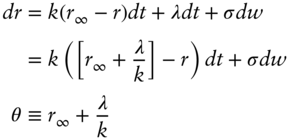
The Vasicek model assumes mean reversion to set the expected path of the short‐term rate. When below its long‐term value, the short‐term rate is expected to increase; when above its long‐term value, the short‐term rate is expected to decrease. Mathematically, the risk‐neutral dynamics for the short‐term rate, ![]() , are given by,
, are given by,
In words, the instantaneous change in the short‐term rate, ![]() , is determined by a trend or drift plus a random fluctuation or shock. The drift is equal to the parameter of mean reversion,
, is determined by a trend or drift plus a random fluctuation or shock. The drift is equal to the parameter of mean reversion, ![]() , times the distance between the long‐run value of the short‐term rate,
, times the distance between the long‐run value of the short‐term rate, ![]() , and its current value. Because all variables are expressed in annualized terms, the
, and its current value. Because all variables are expressed in annualized terms, the ![]() factor adjusts for the actual passage of time. Say, for example, that
factor adjusts for the actual passage of time. Say, for example, that ![]() ;
; ![]() , and
, and ![]() . Then the drift of the short‐term rate in Equation (9.1) is
. Then the drift of the short‐term rate in Equation (9.1) is ![]() or 0.1485% or 14.85 basis points per year. The drift over a month, therefore, with
or 0.1485% or 14.85 basis points per year. The drift over a month, therefore, with ![]() , would be
, would be ![]() or about 1.2 basis points per month. The shock around the drift in Equation (9.1) is
or about 1.2 basis points per month. The shock around the drift in Equation (9.1) is ![]() , where
, where ![]() is a normally distributed random variable with mean equal to zero and standard deviation equal to
is a normally distributed random variable with mean equal to zero and standard deviation equal to ![]() . The shock, therefore, is normally distributed with mean zero and standard deviation
. The shock, therefore, is normally distributed with mean zero and standard deviation ![]() . For example, if
. For example, if ![]() is 0.95%, or 95 basis points per year, then the volatility of the shock over a month is
is 0.95%, or 95 basis points per year, then the volatility of the shock over a month is ![]() basis points.
basis points.
As explained in the previous chapter, fixed income security prices may incorporate a risk premium that is indistinguishable from a drift in the evolution of the short‐term rate. Along these lines, Equation (9.1) can be viewed as containing a drift due to a risk premium. Assume for the purposes of this section that the risk premium is a known constant of ![]() basis points per year, and that the long‐run value of the short‐term rate under the true or real‐world probabilities is
basis points per year, and that the long‐run value of the short‐term rate under the true or real‐world probabilities is ![]() . In that case, the true process of the short‐term rate with the addition of a drift due to the risk premium is,
. In that case, the true process of the short‐term rate with the addition of a drift due to the risk premium is,
(9.3)
Equation (9.3) neatly emphasizes the inability to distinguish expectations from risk premium by observing security prices: an infinite number of combinations of ![]() and
and ![]() give the same
give the same ![]() and, therefore, the same risk‐neutral price process in Equation (9.1).
and, therefore, the same risk‐neutral price process in Equation (9.1).
One reason that the Vasicek model is useful, both for learning about term structure models and for some simple pricing and hedging applications, is that most rates and prices from the model can be expressed through simple formulae. For the most complex securities, numerical methods, like binomial trees, are needed, and Appendix A9.1 explains how the model's dynamics might be captured in a binomial tree. The text, however, continues by presenting analytic solutions of the model, of which some of the most useful are,
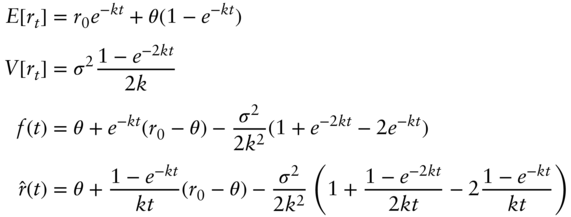
where ![]() gives today's expectation of the short‐term rate at time t,
gives today's expectation of the short‐term rate at time t, ![]() gives the variance of the short‐term rate at time
gives the variance of the short‐term rate at time ![]() ,
, ![]() is the continuously compounded forward rate of term
is the continuously compounded forward rate of term ![]() ; and
; and ![]() is the continuously compounded spot rate of term
is the continuously compounded spot rate of term ![]() .
.
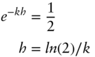
Figures 9.1 through 9.3 illustrate these formulae with the parameter values given earlier. The expected short‐term rate, according to Equation (9.4) and the solid line in Figure 9.1, moves gradually from ![]() today (
today (![]() ) to
) to ![]() in the very distant future (
in the very distant future (![]() ). The mean reversion parameter governing the speed of that adjustment,
). The mean reversion parameter governing the speed of that adjustment, ![]() , is sometimes quoted instead as a half‐life. From Equation (9.4), a shock to
, is sometimes quoted instead as a half‐life. From Equation (9.4), a shock to ![]() decays according to the factor
decays according to the factor ![]() . And half of such a shock decays away after time
. And half of such a shock decays away after time ![]() , such that,
, such that,
For the relatively small mean reverting parameter, ![]() ,
, ![]() is over 42 years, which means that any shock to
is over 42 years, which means that any shock to ![]() affects rate expectations over a very long period of time. Equivalently, the expected rate takes a very long time to revert from the current rate to
affects rate expectations over a very long period of time. Equivalently, the expected rate takes a very long time to revert from the current rate to ![]() .
.
The standard deviation of the short‐term rate around its expectations is given by the square root of (9.5) and shown by the dashed lines in Figure 9.1. With a volatility parameter of 95 basis points per year and a very slow mean reversion, the standard deviation around expectations is quite wide. The figure does show, however, that mean reversion narrows this standard deviation. Without mean reversion, the standard deviation of the short‐term rate is greater, at ![]() . Put another way, the pull of the short‐term rate to the constant value
. Put another way, the pull of the short‐term rate to the constant value ![]() reduces the standard deviation of the short‐term rate as of any future date.
reduces the standard deviation of the short‐term rate as of any future date.
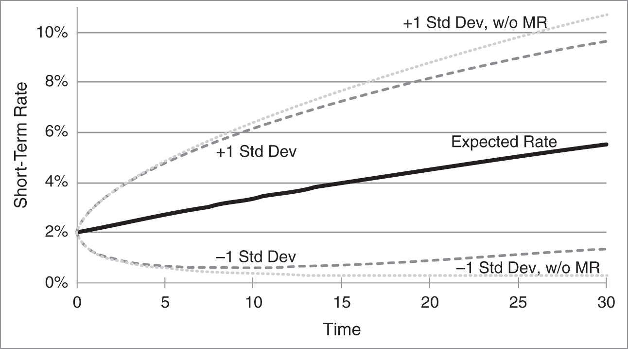
FIGURE 9.1 Expectations of the Continuously Compounded Short‐Term Rate in the Vasicek Model, with One‐Standard‐Deviation Bands. Light Dotted Lines Give Bands Without Any Mean Reversion. Model Parameters Are  ,
,  ,
,  , and
, and  .
.
Equations (9.6) and (9.7), illustrated in Figure 9.2, give the continuously compounded forward and spot rates in the model. The shape of the forward curve is discussed presently. Recall, however, as discussed in Chapter 2, so long as the forward curve is above the spot curve, spot rates are increasing.
Figure 9.3 shows the term structure of forward rate volatility in the model, that is, the instantaneous volatility of forward rates of different terms. Because the only volatility in the model is the volatility of changes in the short‐term rate, the volatility of ![]() – from Equation (9.6) – is just
– from Equation (9.6) – is just ![]() . The mean reversion feature of the model, therefore, captures the empirical regularity that, for longer terms, the term structure of volatility is downward sloping. Empirical volatilities of short‐term rates are much lower than indicated in this figure, however, because the central bank pegs short‐term rates. The Gauss+ model, discussed next, has the flexibility to capture both a low short‐term rate volatility and an ultimately declining term structure of volatilities. In any case, note from Equation (9.6) that the sensitivity of each forward rate to changes in the short‐term rate is
. The mean reversion feature of the model, therefore, captures the empirical regularity that, for longer terms, the term structure of volatility is downward sloping. Empirical volatilities of short‐term rates are much lower than indicated in this figure, however, because the central bank pegs short‐term rates. The Gauss+ model, discussed next, has the flexibility to capture both a low short‐term rate volatility and an ultimately declining term structure of volatilities. In any case, note from Equation (9.6) that the sensitivity of each forward rate to changes in the short‐term rate is ![]() . Hence, these sensitivities across terms have the same shape as in Figure 9.3.
. Hence, these sensitivities across terms have the same shape as in Figure 9.3.
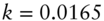
Figure 9.4, the last presented on the Vasicek model, decomposes the forward rate curve into expectations, risk premium, and convexity using the values ![]() , which – given
, which – given ![]() and Equation (9.3) – means that
and Equation (9.3) – means that ![]() . In this decomposition, expectations are mildly increasing over the coming years. Forward rates out to 10 year or so increase much more rapidly than expectations, however, due to the risk premium of 12.5 basis points per year. For longer terms, however, the (negative) convexity term grows rapidly, not only moderating the impacts of expectations and convexity but also actually causing forward rates to decline with term.
. In this decomposition, expectations are mildly increasing over the coming years. Forward rates out to 10 year or so increase much more rapidly than expectations, however, due to the risk premium of 12.5 basis points per year. For longer terms, however, the (negative) convexity term grows rapidly, not only moderating the impacts of expectations and convexity but also actually causing forward rates to decline with term.
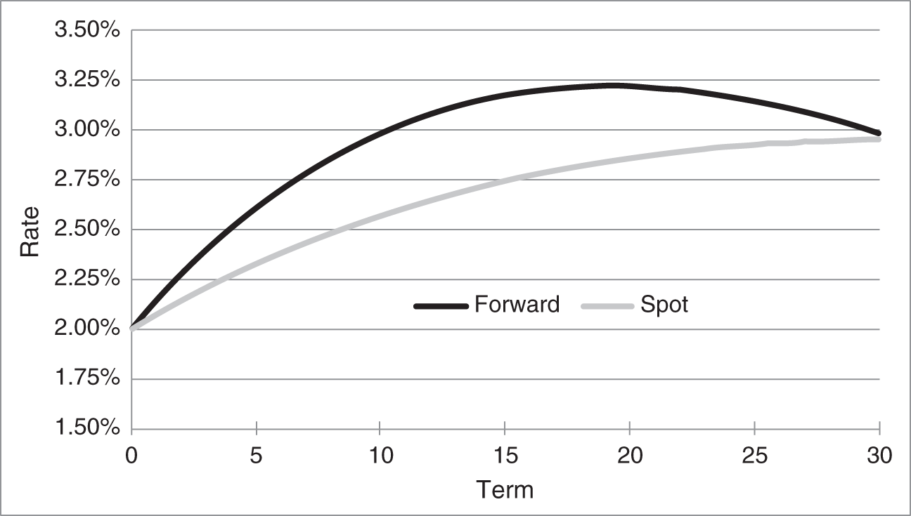
FIGURE 9.2 Continuously Compounded Forward and Spot Rates in the Vasicek Model. Model Parameters Are  ,
,  ,
,  , and
, and  .
.
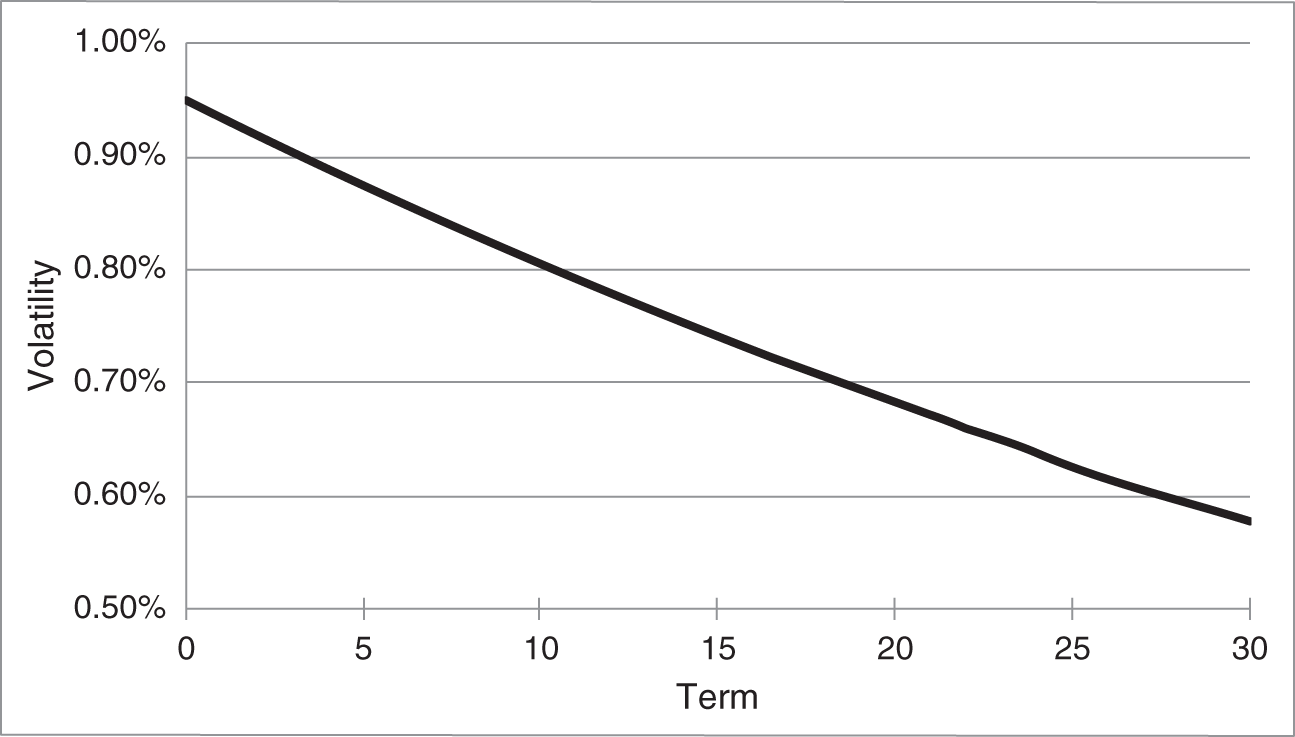
FIGURE 9.3 Term Structure of Forward Rate Volatilities in the Vasicek Model. Parameters Are  ,
,  ,
,  , and
, and  .
.
FIGURE 9.4 Decomposition of the Forward Rates in the Vasicek Model into Expectations, Risk Premium, and Convexity. Model Parameters Are  ,
,  ,
,  ,
,  , and
, and  .
.
The Vasicek model has some limited uses for practitioners. It is a relatively simple model, which is a great advantage. Furthermore, as explained in Chapter 6, a single factor can explain a large fraction of term structure variability, particular across longer maturities. The parameters ![]() ,
, ![]() , and
, and ![]() can be jointly calibrated to approximate both the shape of the term structure and the shape of rate sensitivities to the factor (i.e., Figure 9.3). The parameter
can be jointly calibrated to approximate both the shape of the term structure and the shape of rate sensitivities to the factor (i.e., Figure 9.3). The parameter ![]() can be used to approximate an implied option volatility at one point of the term structure. With these considerations in mind, the model can reasonably be used, for example, to price, compare values, and hedge long‐term bonds that are first callable after some intermediate number of years. The model is flexible enough to match the prices of noncallable bonds from 10 to 30 years, and also to match the most relevant volatility, namely, the volatility of 10‐year rates. Bond sensitivities to changes in interest rates, defined in the model as changes in
can be used to approximate an implied option volatility at one point of the term structure. With these considerations in mind, the model can reasonably be used, for example, to price, compare values, and hedge long‐term bonds that are first callable after some intermediate number of years. The model is flexible enough to match the prices of noncallable bonds from 10 to 30 years, and also to match the most relevant volatility, namely, the volatility of 10‐year rates. Bond sensitivities to changes in interest rates, defined in the model as changes in ![]() , can be computed by shifting
, can be computed by shifting ![]() , recomputing prices, and computing DV01s or durations. To the extent that bonds of one maturity are hedged with bonds of another maturity, the effectiveness of the resulting hedges depend on the reliability of the shape in Figure 9.3.
, recomputing prices, and computing DV01s or durations. To the extent that bonds of one maturity are hedged with bonds of another maturity, the effectiveness of the resulting hedges depend on the reliability of the shape in Figure 9.3.
The model might also be used for trading and hedging relatively long‐term bonds. The value of ![]() might be set each day so that the model 10‐year rate matches the market 10‐year rate. Deviations of calculated prices of longer‐term bonds from model predictions might then be taken as signals of relative value, with hedge ratios calculated as described in the previous paragraph. The success of relative value trading along these lines depends on the extent to which the model captures the equilibrium or steady state of the shape of the term structure. Also, as before, hedging effectiveness depends on the reliability of the term structure of sensitivities to the factor.
might be set each day so that the model 10‐year rate matches the market 10‐year rate. Deviations of calculated prices of longer‐term bonds from model predictions might then be taken as signals of relative value, with hedge ratios calculated as described in the previous paragraph. The success of relative value trading along these lines depends on the extent to which the model captures the equilibrium or steady state of the shape of the term structure. Also, as before, hedging effectiveness depends on the reliability of the term structure of sensitivities to the factor.
The Vasicek model is not very widely used, however, because it is too simple for most applications. First, the model is not flexible enough to approximate the wide variety of observed market term structures. Or, put another way, calibrating the model to match one point on the term structure relies too heavily on the model to approximate all other points on the term structure. Second, while one factor does explain a lot of term structure variability, a second factor can capture significantly more variability. In terms of the discussion in Chapter 6, more than one factor is needed to hedge intermediate‐ and shorter‐term bonds. Third, the Vasicek model cannot capture the empirical regularity, mentioned already, that the term structure of volatilities and, therefore, the term structure of factor sensitivities, typically rises quickly with term and then flattens or declines. This limitation means that the model cannot simultaneously handle options or other volatility‐sensitive products that are spread out across the term structure, nor can it reliably hedge bonds most sensitive to one segment of the term structure with bonds most sensitive to another segment. With these caveats, the text turns to a much more flexible term structure model.
9.2 THE GAUSS+ MODEL
The Gauss+ model is well‐known among practitioners as a tool for proprietary trading and hedging. The assumptions of the model are intuitively appealing, and they reasonably balance the goals of tractability and of capturing the empirical complexity of term structure dynamics. The goal of the text is to introduce the model, both in theory – through its equations and solution – and in application – through a full estimation of its parameters using recent data. Introducing a detailed estimation procedure here is noteworthy, because methodologies across the industry vary widely. The goal of the extensive appendix to this section is to enable a determined reader to estimate and implement the model independently.
The dynamics of the cascade form of the model are given in Equations (9.9) through (9.12). The factors ![]() ,
, ![]() , and
, and ![]() denote the short‐term rate of interest, a medium‐term factor, and a long‐term factor, respectively. The parameters
denote the short‐term rate of interest, a medium‐term factor, and a long‐term factor, respectively. The parameters ![]() and
and ![]() are discussed presently. The mean reversion parameters of the factors are,
are discussed presently. The mean reversion parameters of the factors are, ![]() ,
, ![]() , and
, and ![]() , respectively, and the volatility parameters for the medium‐ and long‐term factors are
, respectively, and the volatility parameters for the medium‐ and long‐term factors are ![]() and
and ![]() , respectively. The two random variables in the model are
, respectively. The two random variables in the model are ![]() and
and ![]() . The subscript
. The subscript ![]() denotes time‐
denotes time‐![]() observations of the factors, of changes in the factors, and of the random variables. Finally, then, the equations are,
observations of the factors, of changes in the factors, and of the random variables. Finally, then, the equations are,
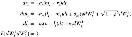
Given the structure of the model, it turns out that the medium‐ and long‐term factors can be thought of as rates. The short‐term rate mean reverts to the medium‐term factor, which is meant to reflect business cycles and monetary policy factors. The medium‐term factor reverts to the long‐term factor, which is meant to reflect long‐term expectations of inflation and the real interest rate, which ultimately depend on long‐term trends in demographics, production technology, and so forth. And the long‐term factor reverts to a constant, ![]() , which, as in the Vasicek model, can be thought of as including both a long‐term expectation of the short‐term rate and a risk premium. The mean reversion parameters are expected to be consistent with these economic interpretations; that is, the short‐term rate reverts quickly to the medium‐term factor; the medium‐term factor reverts more slowly to the long‐term factor; and the long‐term factor reverts slowest of all to its target.
, which, as in the Vasicek model, can be thought of as including both a long‐term expectation of the short‐term rate and a risk premium. The mean reversion parameters are expected to be consistent with these economic interpretations; that is, the short‐term rate reverts quickly to the medium‐term factor; the medium‐term factor reverts more slowly to the long‐term factor; and the long‐term factor reverts slowest of all to its target.
While the medium‐ and long‐term factors trend as described in the previous paragraph, they also fluctuate around these trends. With respect to the evolution of the long‐term factor in Equation (9.11), the fluctuation over a short time ![]() is
is ![]() . Because
. Because ![]() is normally distributed with mean zero and standard deviation
is normally distributed with mean zero and standard deviation ![]() , the instantaneous fluctuation of the long‐term factor around its trend has mean zero and volatility
, the instantaneous fluctuation of the long‐term factor around its trend has mean zero and volatility ![]() . The random terms in Equation (9.10) look complicated, but they simply ensure that the instantaneous fluctuation of the medium‐term factor around its trend has a volatility of
. The random terms in Equation (9.10) look complicated, but they simply ensure that the instantaneous fluctuation of the medium‐term factor around its trend has a volatility of ![]() and a correlation of
and a correlation of ![]() with the fluctuation of the long‐term factor around its trend. To see this, note that
with the fluctuation of the long‐term factor around its trend. To see this, note that ![]() also has mean zero and standard deviation
also has mean zero and standard deviation ![]() , and, from Equation (9.12), zero correlation with
, and, from Equation (9.12), zero correlation with ![]() . It then follows from Equation (9.10) that the standard deviation of
. It then follows from Equation (9.10) that the standard deviation of ![]() is,
is,
that the covariance of ![]() and
and ![]() is,
is,
and, therefore, that the correlation of ![]() and
and ![]() is,
is,
The evolution of the short‐term rate in the model, Equation (9.9), is meant to reflect how central banks conduct rate policy. The Fed, for example, keeps the short‐term policy rate pegged or fixed at a target, but moves that target over time in a manner deemed appropriate for the state of the business cycle and monetary conditions. Mathematically, in Equation (9.9), the short‐term rate is fixed over the very short time interval, ![]() , in the sense that there is no random variable shocking the dynamics of
, in the sense that there is no random variable shocking the dynamics of ![]() . The rate,
. The rate, ![]() , is pushed gradually, however, toward the medium‐term factor,
, is pushed gradually, however, toward the medium‐term factor, ![]() , which in turn reverts to the long factor,
, which in turn reverts to the long factor, ![]() .
.
The medium‐ and long‐term factors move expectations of the short‐term rate as of future dates. Because these expectations move smoothly over time, the medium‐ and long‐term factors are assumed to move in a continuous fashion. The short‐term rate, by contrast, changes in the real world by discrete amounts, on a set of fixed dates, according to central bank policy decisions. The model approximates the future outcomes of this process, however, by a continuous process starting at today's short‐term rate.
The lack of a volatility term in Equation (9.9) is an important feature of the Gauss+ model. As pointed out in the discussion of the Vasicek model, mean‐reverting factors generate a downward‐sloping term structure of volatility. Largely because of central banks, however, empirical and implied term structures of volatility tend to have a hump; that is, volatility is low for very short‐term rates before increasing to a peak at intermediate‐term or longer rates. In the Gauss+ model, the lack of a random shock in the dynamics of ![]() keeps short‐term rate volatility low. In this way, the Gauss+ model can match empirically observed hump‐shaped term structures of volatility.
keeps short‐term rate volatility low. In this way, the Gauss+ model can match empirically observed hump‐shaped term structures of volatility.
In passing, the Gauss+ model gets its name from the lack of a volatility term in Equation (9.9). The “Gauss” part of the name indicates that interest rates have a normal or Gaussian distribution. But while most one‐, two‐, or three‐factor normal models have a corresponding number of sources of risk, the Gauss+ model, strictly speaking, has three factors, but only two sources of risk. The model has three state variables in the sense that describing the state of the world in the model requires knowing the three factors, ![]() ,
, ![]() , and
, and ![]() . There are only two sources of risk, however, namely,
. There are only two sources of risk, however, namely, ![]() and
and ![]() . The “+” in the name, therefore, indicates the somewhat unusual presence of a factor or state variable that is not also a source of risk.
. The “+” in the name, therefore, indicates the somewhat unusual presence of a factor or state variable that is not also a source of risk.
As a final comment on the structure of the model, Equations (9.9) through (9.12) are the risk‐neutral dynamics of the model. Additional assumptions allow for the identification of an implicit risk premium. An application of the model developed next shows how this may be done, assuming that only the long‐term factor earns a risk premium.2
Appendix A9.2 gives a detailed account of how the parameters of the Gauss+ model might be estimated from bond or swap data. A simplified overview is presented here, using daily data from January 2014 to January 2022 on the fed funds target rate (see Chapter 12) and on zero coupon bond prices of various maturities, which are derived from the prices of US Treasury bonds. The time series of zero coupon bond prices are published by the Federal Reserve Bank of New York and are publicly available.3
Consistent with the interpretation of the model, the short‐term rate, ![]() , is taken each day as equal to the fed funds target rate on that day. While a general collateral repo rate is theoretically more consistent with a term structure of Treasury interest rates, repo rates exhibit occasional idiosyncratic jumps that complicate the estimation without significant offsetting advantages.
, is taken each day as equal to the fed funds target rate on that day. While a general collateral repo rate is theoretically more consistent with a term structure of Treasury interest rates, repo rates exhibit occasional idiosyncratic jumps that complicate the estimation without significant offsetting advantages.
Once estimated, the model factors are chosen to “fit” or match, each day, the one‐year rates, two and 10 years forward, and the fed funds target rate. Furthermore, as discussed presently, with these two‐ and 10‐year forward rates fair by construction, the model becomes a tool for trading value in other parts of the curve relative to these fitted points. For ease of exposition, by the way, all forward rates mentioned from this point denote one‐year rates some number of years forward.
Although the model ultimately fits the two‐ and 10‐year forward rates, note that the factors ![]() and
and ![]() are in no way those forward rates themselves, in the way that
are in no way those forward rates themselves, in the way that ![]() equals the fed funds rate. The relationships of all forward rates to
equals the fed funds rate. The relationships of all forward rates to ![]() and
and ![]() depend on the estimated model parameters and, in particular, on the mean reversion parameters. More specifically, the larger
depend on the estimated model parameters and, in particular, on the mean reversion parameters. More specifically, the larger ![]() , the faster changes to the factors
, the faster changes to the factors ![]() and
and ![]() make their way into the term structure of rates. The larger
make their way into the term structure of rates. The larger ![]() , the faster
, the faster ![]() converges to
converges to ![]() , and the less
, and the less ![]() affects longer‐term yields. And the smaller
affects longer‐term yields. And the smaller ![]() , the slower
, the slower ![]() converges to
converges to ![]() , and the more similar or parallel is the effect of
, and the more similar or parallel is the effect of ![]() on all longer‐term yields.
on all longer‐term yields.
9.3 A PRACTICAL ESTIMATION METHOD
The estimation method presented here proceeds in stages, with each stage estimating a subset of the model's parameters.4
Figure 9.5 shows the coefficients of regressing the changes in the zero yields of various terms on changes in the two‐year zero yield – the dark gray bars – and on changes in the 10‐year zero yield – the light gray bars. For example, the regression of the three‐year yield gives a coefficient of 0.91 on the two‐year yield and 0.22 on the 10‐year yield. By contrast, the regression of the 15‐year yield gives a coefficient of ![]() 0.20 on the two‐year yield and 1.10 on the 10‐year yield. In any case, as explained before, all these regression coefficients implicitly describe the mean reversion parameters of the model. This stage of the estimation, therefore, chooses the parameters
0.20 on the two‐year yield and 1.10 on the 10‐year yield. In any case, as explained before, all these regression coefficients implicitly describe the mean reversion parameters of the model. This stage of the estimation, therefore, chooses the parameters ![]() ,
, ![]() , and
, and ![]() so that the model captures the empirically observed regression coefficients as closely as possible. This staging is possible, because, as shown in the appendix, the model regression coefficients depend only on the mean reversion parameters, not on the volatility parameters. In any case, the mottled dark and light gray bars in Figure 9.5 show the success of this stage of the estimation. There are a set of mean reversion parameters, given hereafter, such that implied regression coefficients from the model very closely match the empirically observed regression coefficients. And, while not reported here, these matches are within statistical confidence intervals.
so that the model captures the empirically observed regression coefficients as closely as possible. This staging is possible, because, as shown in the appendix, the model regression coefficients depend only on the mean reversion parameters, not on the volatility parameters. In any case, the mottled dark and light gray bars in Figure 9.5 show the success of this stage of the estimation. There are a set of mean reversion parameters, given hereafter, such that implied regression coefficients from the model very closely match the empirically observed regression coefficients. And, while not reported here, these matches are within statistical confidence intervals.
The next stage of the estimation is to find the volatility and correlation parameters, ![]() ,
, ![]() , and
, and ![]() , so that the term structure of volatilities in the model matches the term structure of volatilities in the data as closely as possible. The result of this optimization is shown in Figure 9.6. Once again, the model is flexible enough to do an excellent job of matching empirical properties of the term structure of interest rates.
, so that the term structure of volatilities in the model matches the term structure of volatilities in the data as closely as possible. The result of this optimization is shown in Figure 9.6. Once again, the model is flexible enough to do an excellent job of matching empirical properties of the term structure of interest rates.
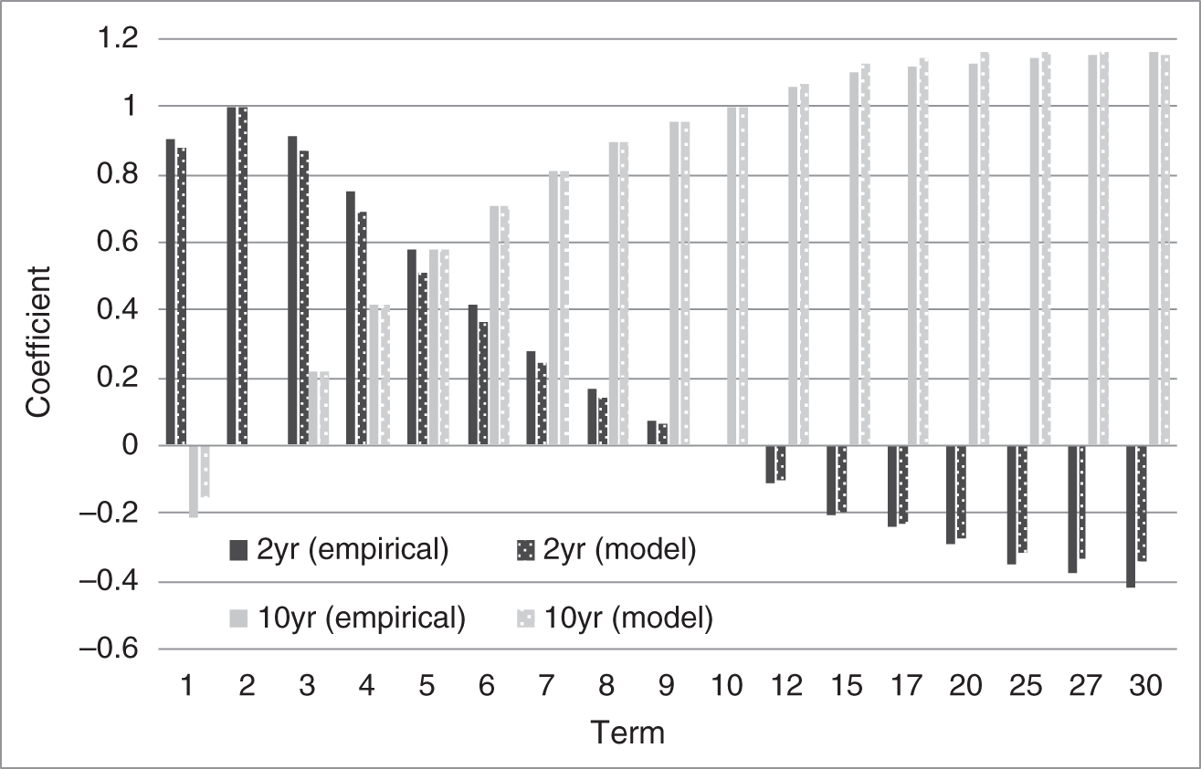
FIGURE 9.5 Coefficients of Regressing Zero Coupon Bond Yields of Various Terms on Two‐ and 10‐Year Zero Coupon Bond Yields, from Empirical Analysis and as Implied by the Estimated Gauss+ Model.
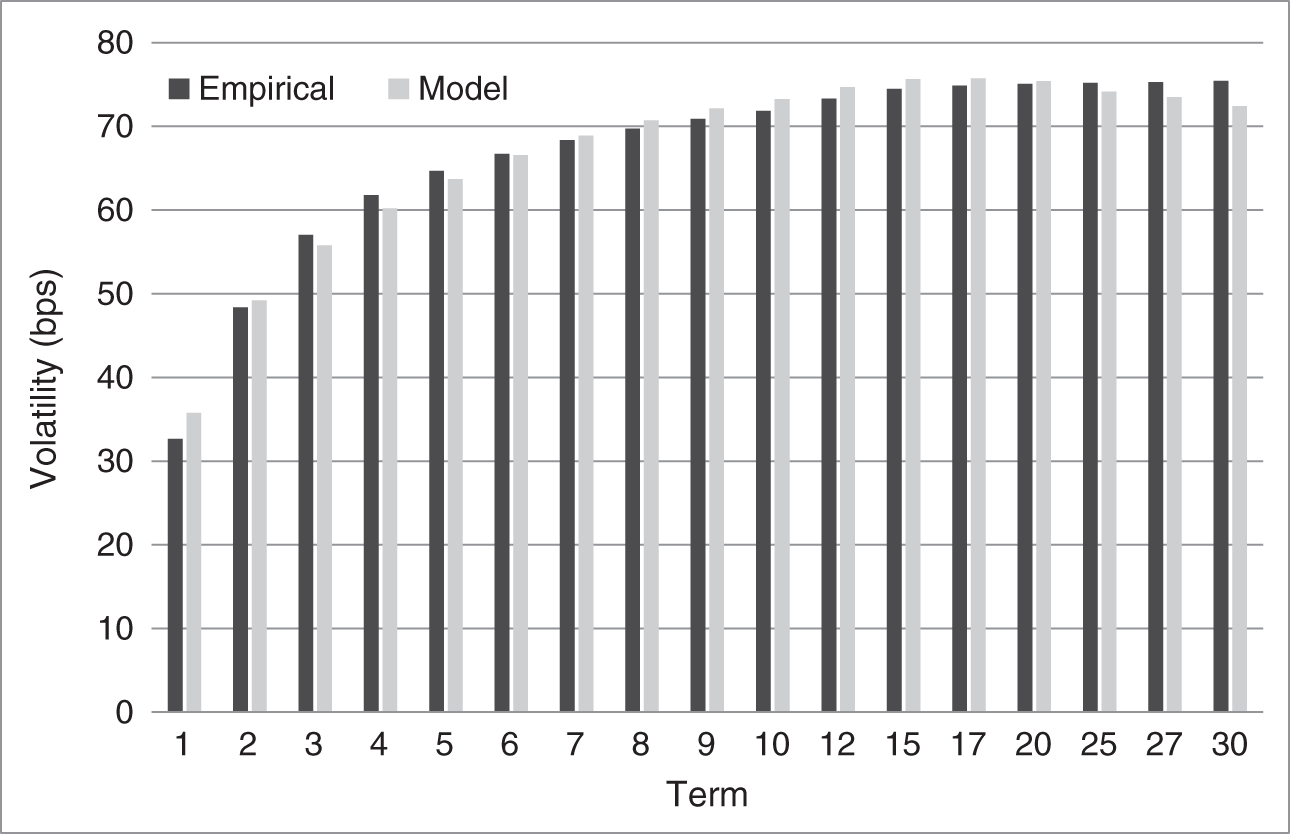
FIGURE 9.6 Yield Volatility in Annual Basis Points, from Empirical Analysis and as Implied by the Estimated Gauss+ Model.
The last remaining parameter to be estimated is ![]() , the value to which the short‐term rate reverts, over the very long‐term. The estimation procedure suggested here finds the
, the value to which the short‐term rate reverts, over the very long‐term. The estimation procedure suggested here finds the ![]() that minimizes the sum of the squared errors of observed yields relative to model yields across the whole data sample.
that minimizes the sum of the squared errors of observed yields relative to model yields across the whole data sample.
Following the estimation procedure described, Table 9.1 reports the resulting Gauss+ parameter values. The mean reversion parameters are in the order expected, with the central bank reaction fastest, the speed of the medium‐term factor's reversion to the long‐term factor next, and the speed of the long‐term factor's reversion to ![]() slowest. Alternatively, the time for each process to converge halfway to its target, given in the half‐life column, is about eight months for
slowest. Alternatively, the time for each process to converge halfway to its target, given in the half‐life column, is about eight months for ![]() , 13 months for
, 13 months for ![]() , and 42 years for
, and 42 years for ![]() . Because of the mean reverting nature of the factors, the volatility parameters of 109 and 96 basis points for the medium‐ and long‐term factors, respectively, translate into the lower zero yield volatilities shown in Figure 9.6. The parameter
. Because of the mean reverting nature of the factors, the volatility parameters of 109 and 96 basis points for the medium‐ and long‐term factors, respectively, translate into the lower zero yield volatilities shown in Figure 9.6. The parameter ![]() , as the very long‐run target for the short‐term rate, might seem high at over 10%, but the long‐term factor reverts very slowly to this target, and that target includes a risk premium, which is discussed further next.
, as the very long‐run target for the short‐term rate, might seem high at over 10%, but the long‐term factor reverts very slowly to this target, and that target includes a risk premium, which is discussed further next.
The term‐structure properties of the estimated model are well described by Figure 9.7, which graphs the change in forward rates for a change in each of the factors as a function of term. For example, the seven‐year forward, changes by 0.9 basis points for every basis point change in the long‐term factor. Taken as a whole, the figure shows that short‐term factor affects only the very short end of the curve. The medium‐term factor, which drives the two‐ to three‐year part of the curve, can be thought of as capturing monetary policy in the sense of encapsulating where the market believes the short‐term rate will be in two to three years. The long‐term factor has its biggest impact in six to eight years and, beyond 10 years, is the sole factor driving forward rate changes and volatilities.
The time series properties of the model can be described by graphing its factors over time. As mentioned already, the short‐term rate is set each day to the fed funds target rate, and the medium‐ and long‐term factors are set so as to match the model and market two‐ and 10‐year forward rates. Figure 9.8 graphs these empirically recovered market factors from January 2007 to January 2022.5 The two‐year forward rate is included in the graph to focus the interpretation of the medium‐term factor. When rates are high, this factor closely tracks the two‐year forward rate, confirming that the medium‐term factor loosely corresponds to where the market expects the short‐term rate to be in two years. When rates are low, however, near the zero lower bound, the medium‐term factor can fall into deeply negative territory. In this sense, the medium‐term factor is a “forward shadow rate” that reflects future expectations of the short‐term rate and that can be traded explicitly in the Gauss+ model. This interpretation differs from models in which the “shadow rate” is what the short‐term rate would be now if it were not bounded above zero.6 In any case, the nature of the medium‐rate factor as a leading indicator of the short‐term rate can be seen by comparing those two series in Figure 9.8. Particularly striking is the steep increase in the medium‐term factor starting in early 2014, a couple of years before the Federal Reserve began raising rates.
TABLE 9.1 Estimated Parameters of the Gauss+ Model from US Treasury Zero Coupon Yields, January 2014 to January 2022. Half‐Life Is in Years.
| Parameter | Estimate | Half‐Life |
|---|---|---|
| 1.0547 | 0.66 | |
| 0.6358 | 1.09 | |
| 0.0165 | 42.01 | |
| 109.2 bps | ||
| 96.4 bps | ||
| 0.212 | ||
| 10.555% |
FIGURE 9.7 Changes in Forward Rates Relative to Changes in the Short‐Rate, the Medium‐Term Factor, and the Long‐Term Factor in the Estimated Gauss+ Model.
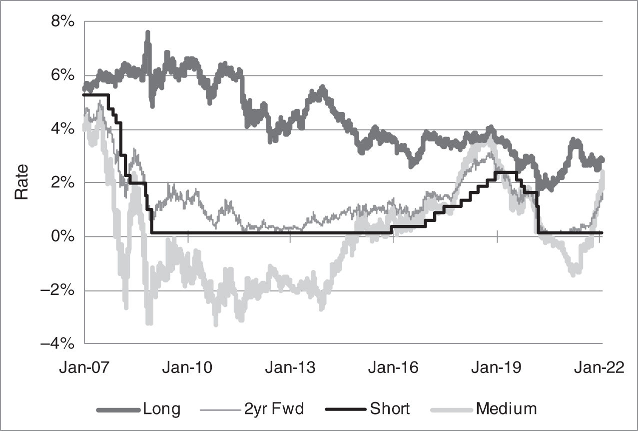
FIGURE 9.8 The Two‐Year Forward Rate and Gauss+ Factors Extracted from Daily Market Data.
9.4 RELATIVE VALUE AND MACRO‐STYLE TRADING WITH THE GAUSS+ MODEL
In the context of a term structure model, a relative value trade is one that is not exposed to or hedged against changes in the factors. Ideally, a trader would find an individual security that is cheap relative to the model and, from various analyses, is expected to revert soon to being fair to the model. The trader would then buy that security; hedge some or all of its factor exposure by selling fair or rich securities in the same part of the curve; and earn the resulting profits. In practice, however, individual securities are often persistently cheap or rich to the model, so that convergence is not expected in the short run, and securities neighboring in term are often all fair or rich together. Most of the time, therefore, relative value opportunities arise in which a trader receives forward rates in one part of the curve that are high relative to the model but expected to converge promptly to the model; pays forward rates in another part of the curve that are too low, but expected to converge promptly; and structures trades to minimize factor exposures. In this synopsis, the speed at which any detected mispricing is likely to correct itself is an important trading consideration.
As an example of using the Gauss+ model along these lines, consider the following framework. Compute the time series of the nine‐year forward rate minus the model‐predicted equivalent rate, where each observation can be called a fitting error. Then construct a signal from this times series as the difference between its five‐day and 40‐day moving averages. If the demeaned fitting error at a given time is positive, so that the nine‐year forward is too high relative to the model, and if the signal is negative, so that fitting errors have started to fall, that is, they have started to converge to the model, then receiving at that forward rate might be considered an attractive trade.
The problem with receiving or paying the nine‐year forward in isolation, however, is that it has significant exposure to the medium‐ and long‐term factors, which is not consistent with the spirit of relative value trading. One solution is to pool together and size several attractive relative value trades so that their exposure to the factors is minimal. In addition, traders can diversify across mean reverting trades. It turns out, for example, that nine‐ and five‐year fitting errors tend to be positively correlated. This fact makes it attractive to pay in one rate and receive in the other. Figure 9.9 shows, in fact, that the difference between the nine‐ and five‐year signals is strongly mean reverting, which is one of the most important properties of relative value trades.
Unlike relative value trading, which finds value in the absence of factor exposure, macro trading takes direct or indirect views on the factors. Simple examples include positions based on predictions of changes in rates or in the slope of the term structure that differ from what is priced in the market. A more complex example, which has attracted more interest over time, is trying to trade the long‐run level of the short‐term rate. As explained earlier, long‐term forward rates are a combination of expectations, risk premium, and convexity. Within the structure of the Gauss+ model, with the help of a strategic assumption, long‐term forward rates can be separated into these three components. A macro trader can then decide that long‐term forwards are too low or too high and position accordingly. The details of this decomposition of forward rates are complex and, therefore, appear in the appendix to this chapter. The text continues with an intuitive approach.
In the context of any term structure model, it is relatively straightforward to determine the effect of convexity on forward rates. It is much more difficult, however, to separate expectations from risk premium. A number of approaches appear in the academic literature, but these are not without various shortcomings.7 The method proposed here relies on one key assumption: expectations of future short‐term rates do not change past some point in the future. Anyone with a view of the short‐term rate in 15 years, for example, has the same view of the short‐term rate in 20 or in 30 years. Consequently, any difference in forward rates beyond some term is attributable not to rate expectations, but solely to risk premium and convexity. In this way, expectations and risk premium can be separated and calculated from observable rates.
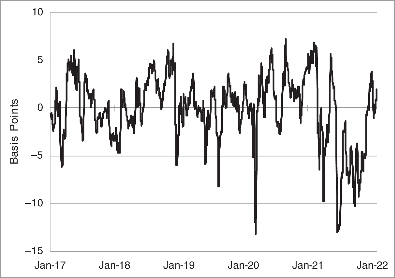
FIGURE 9.9 Difference Between the Nine‐ and Five‐Year Signals. Each Signal Is Based on a Difference of Moving Averages of Deviations of Market from Gauss+ Model Rates.
Using the assumption just described and the parameters of the Gauss+ model estimated previously, Figure 9.10 graphs the risk premium on the 10‐year forward rate over time, measured along the left axis. A value of 60 basis points on any day, for example, means that, on that day, 60 basis points of the 10‐year forward rate is attributable to risk premium. The lighter line is the level of the 10‐year forward rate, measured along the right axis. The risk premium often moves in the opposite direction of rates. As rates decline, the term structure typically steepens, which the model interprets as an increase in risk premium. This observed behavior is consistent with the low‐inflation regime over the last several decades, in which government bond prices increase as other risky assets fall in value. In that environment, as rates fall, and have less room to fall even further, bonds are less able to hedge the declining value of other assets and, as a result, are worth less themselves.
The flip‐side of identifying the risk premium, of course, is identifying the long‐run expectation of the short‐term rate in the estimated Gauss+ model, more specifically, the 10‐year forward rate minus the term‐appropriate risk premium plus the term‐appropriate convexity. The time series of this expectation is shown in Figure 9.11, along with a different estimate, formed from real rate forecasts and inflation estimates at the Federal Reserve Bank of Cleveland.8 While the model and outside series track each other quite well over time, there are trading opportunities to use the difference between the two series as a measure of value. Put another way, the difference between the Gauss+ market‐implied view – the long‐run rate priced in the market – and the exogenous, economist‐generated, fundamental view – what one thinks the long‐run rate should be – can be used as a basis for taking outright long or short positions in bonds.
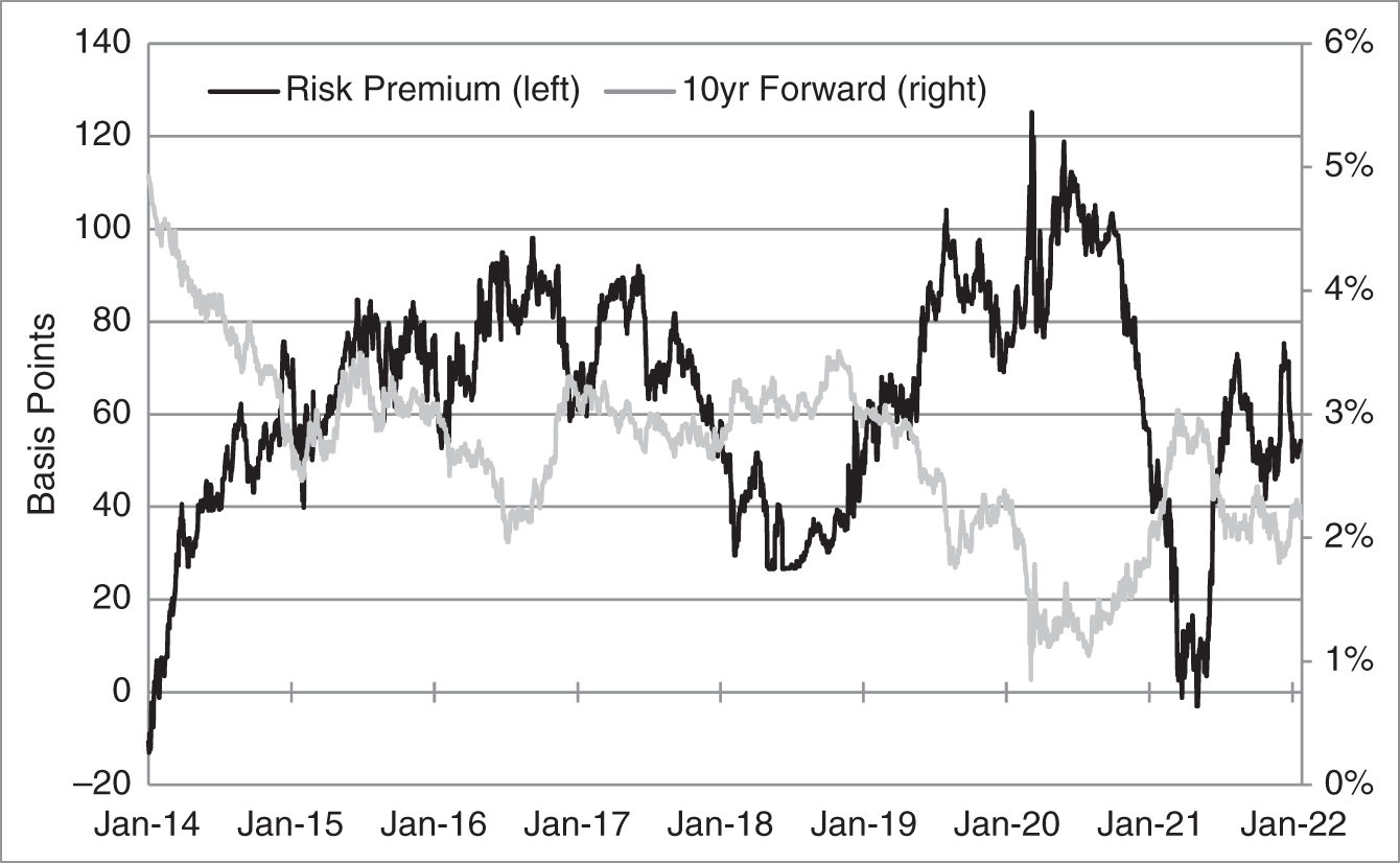
FIGURE 9.10 Estimated Risk Premium on the 10‐Year Forward Rate.
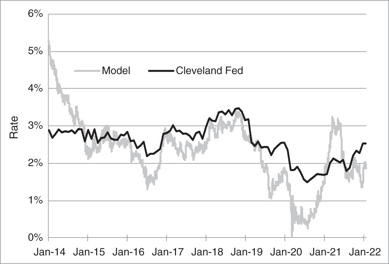
FIGURE 9.11 Long‐Run Expectations of the Short‐Term Rate, as Implied by Gauss+ Fitted to Market Rates and by Fundamental Analysis at the Federal Reserve Bank of Cleveland.
NOTES
- 1 Vasicek, O. (1977),“An Equilibrium Characterization of the Term Structure,” Journal of Financial Economics 5.
- 2 See, for example, Cochrane, J., and Piazzesi, M. (2009), “Decomposing the Yield Curve,” AFA 2010 Atlanta Meetings Paper, January 26.
- 3 See Gürkaynak, R., Sack, B., and Wright, J. (2006), “The US Treasury Yield Curve: 1961 to the Present.” Data are available at https://www.federalreserve.gov/data/nominal‐yield‐curve.html.
- 4 This approach is significantly easier to implement than the maximum likelihood methods that are standard in the term structure literature.
- 5 The model is estimated using data from January 2014, but the resulting parameters are used to extract model factors back through 2007. Also, instead of the long‐term factor itself, the figure graphs the long‐term factor shifted forward 10 years. This allows the series to be more easily interpreted as an approximation for expectations of the short‐term rate in 10 years. See Appendix A9.2 for further details.
- 6 See, for example, Wu, J., and Xia, F. (2016), “Measuring the Macroeconomic Impact of Monetary Policy at the Zero Lower Bound,” Journal of Money Credit and Banking 48, March‐April; Bauer, M., and Rudebusch, G. (2016), “Monetary Policy Expectations at the Lower Bound,” Journal of Money Credit and Banking 48, October; and Kim, D., and Singleton, K. (2012), “Term Structure Models and the Zero Bound: An Investigation of Japanese Yields,” Journal of Econometrics 170, September.
- 7 See, for example, Adrian, T., Crump, R., and Moench, E. (2013), “Pricing the Term Structure with Linear Regressions,” Journal of Financial Economics 110(1), October; Ang, A., and Piazzesi, M. (2003), “A No‐Arbitrage Vector Autoregression of Term Structure Dynamics with Macroeconomic and Latent Variables,” Journal of Monetary Economics 50(4); Cieslak, A. (2018), “Short‐Rate Expectations and Unexpected Returns in Treasury Bonds,” Review of Financial Studies 31(9); and Kim, D., and Orphanides, A. (2012), “Term Structure Estimation with Survey Data on Interest Rate Forecasts,” Journal of Financial and Quantitative Analysis 47(1).
- 8 The construction of the Cleveland Fed series is described further in the appendix to this chapter.