
CHAPTER 11
Note and Bond Futures
Futures on government bonds are among the most liquid fixed income products around the world, used to hedge interest rate risk and to take positions on changes in bond prices. Figure 11.1 shows how the total DV01 traded across all US Treasury bonds and futures is divided across instruments.1 By this metric, the 10‐year note futures contract is the single instrument with the greatest volume, and volumes traded in other futures contracts rival those of on‐the‐run Treasury securities. Futures contracts are appealing because of their liquidity, and also because relatively little cash is required to establish sizable positions. The US Treasury futures discussed in this chapter trade on the CBOT (Chicago Board of Trade), which is part of the CME Group.
A forward contract on a bond is an agreement that fixes the price at which a bond is to be bought and sold on some future date. Forward contracts on bonds are rarely traded in the United States, because, as is shown next, the same economics can be achieved by trading bonds and repo. Understanding forward contracts is important, however, because futures are essentially forwards with the complexities of daily settlement and various delivery options. This chapter, therefore, first describes forward contracts and then adds these features of futures contracts. The exposition includes a discussion of basis trades, in which futures are traded against synthetic forward bond positions, and the chapter concludes with a case study about basis trades through the volatility of March 2020, at the start of the COVID pandemic and economic shutdowns.
For concreteness in explaining concepts, this chapter focuses on the 10‐year US Treasury note contract. Other US bond futures are similar, as are many government bond futures around the world. Contracts on UK and Chinese government bonds, for example, are particularly similar to those in the United States in that they embed both quality and timing options. Contracts on government bonds in Europe and Japan are also similar, but simpler, in that they do not have a timing option.
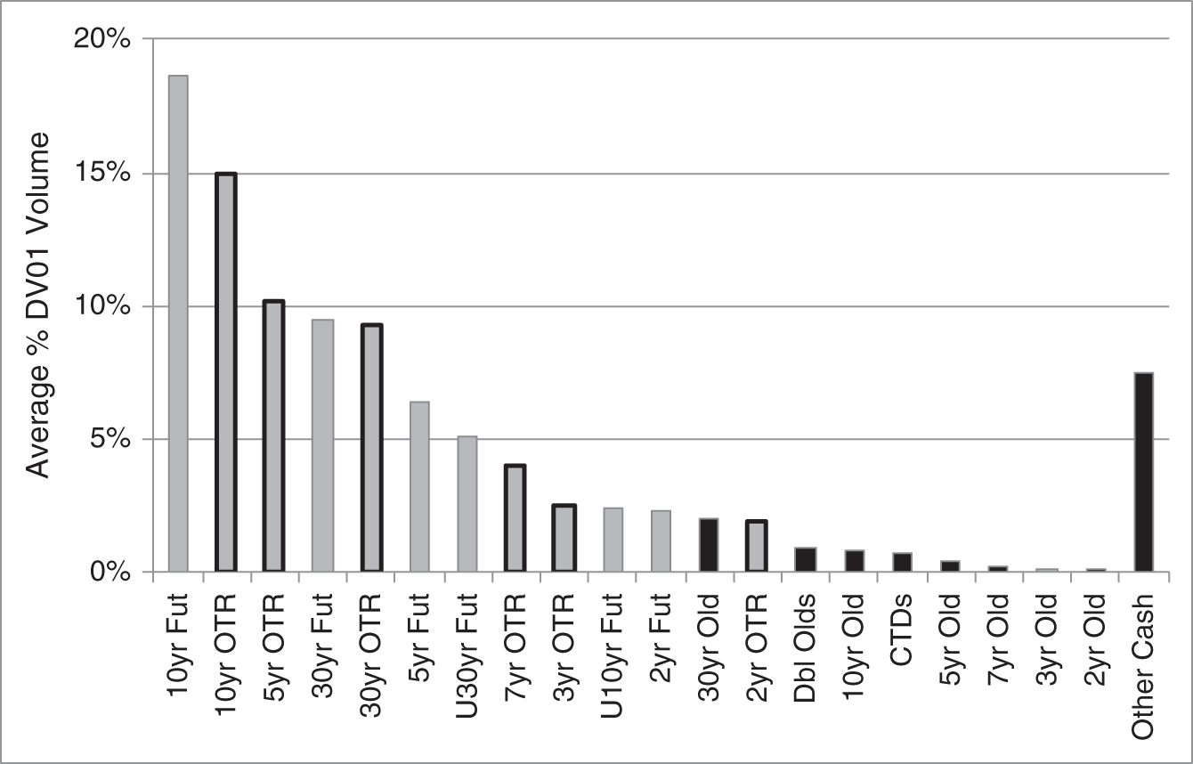
FIGURE 11.1 Percent of Total DV01 Traded in US Treasury Bonds and in US Treasury Note and Bond Futures, by Instrument, from July 10, 2017, to June 1, 2018. “Fut” Denotes Futures Contracts on Bonds of Various Maturities; and “U30yr Fut” and “U10yr Fut” Are the “Ultra” 30‐ and 10‐year Futures Contracts. “OTR” Denotes the On‐the‐Run or Most Recently Issued Treasury Bond at a Given Maturity; “Old” Denotes the Next Most Recent; and “Dbl Old” Denotes the Most Recent After the Old. “CTDs” Denote the Cheapest‐to‐Deliver Bonds into Futures Contracts. “Other Cash” Denotes All Other Treasury Bonds.
Appendix A11.2 outlines the pricing of forward and futures contracts on bonds in a term structure model.
11.1 FORWARD CONTRACTS AND FORWARD PRICES
In a forward bond contract, the counterparties agree on a price at which to trade a bond at some time in the future. Consider a forward contract, traded on May 14, 2021, to purchase $100,000 face amount of the US Treasury 2.875s of 05/15/2028 for 109.72 on September 30, 2021. In this example, the initiation or trade date is May 14, 2021; the underlying security is the 2.875s of 05/15/2028; the forward date, expiration date, delivery date, or maturity date is September 30, 2021; and the forward price is 109.72. The counterparty committing to purchase the bond on the forward date is the buyer of the contract and is long the forward, while the counterparty on the other side is the seller of the contract and is short the forward. Table 11.1 summarizes the terms of this forward trade and gives other data that are used presently.
TABLE 11.1 A Forward Contract on the US Treasury 2.875s of 05/15/2028.
| Underlying Security | 2.875s of 05/15/2028 |
| Principal Amount | $100,000 |
| Trade Date | 05/14/2021 |
| Spot Settlement Date | 05/17/2021 |
| Spot Price | 110.77344 |
| Accrued Interest, Spot Settlement (2/184 days) | 0.01562 |
| Forward Settlement Date | 09/30/2021 |
| Accrued Interest, Forward Settlement (138/184 days) | 1.07813 |
| Repo Rate to Forward Settlement Date | 0.015% |
| Days from Spot to Forward Settlement | 136 |
| Forward Price | 109.71721 |
By definition, the forward price is such that the buyer and seller are willing to enter into the forward agreement without any exchange of cash. This implies that the initial value of the forward contract is zero. Over time, however, the value of the forward position may rise or fall. Continuing with the example, say that, just after the agreement was struck, the market forward price increases to 110. The contract to buy the bond at 109.72 now has positive value to the buyer and negative value to the seller. The buyer could immediately sell the bond through a new forward contract at 110, which makes the contract worth ![]() , or 0.28, as of 09/30/2021, or the present value of 0.28 as of today. The seller of the original contract, however, having locked in a forward price of 109.72, would have to pay the buyer to exit the contract. In any case, note that the “value of a forward contract” denotes the value of an existing contract under current market conditions, while the “forward price” denotes the price at which the underlying bond is to be traded on the forward date.2
, or 0.28, as of 09/30/2021, or the present value of 0.28 as of today. The seller of the original contract, however, having locked in a forward price of 109.72, would have to pay the buyer to exit the contract. In any case, note that the “value of a forward contract” denotes the value of an existing contract under current market conditions, while the “forward price” denotes the price at which the underlying bond is to be traded on the forward date.2

FIGURE 11.2 A Forward Contract on the US Treasury 2.875s of 05/15/2028.
Forward bond prices can be determined by arbitrage arguments. To demonstrate, consider the following strategy in the context of the example, using the data in Table 11.1 and referring to the timeline in Figure 11.2:
On May 14, 2021:
- Buy $100,000 face amount of the 2.875s of 05/15/2028 for 110.77344 plus accrued interest of 0.01562, for settlement on May 17, 2021, for an invoice price of 110.78906 and a dollar invoice of $110,789.06.
- Sell the repo to the forward date, that is, borrow $110,789.06 from May 17, 2021, to September 30, 2021, at the repo rate of 0.015%, and post the 2.875s of 05/15/2028 as collateral.
- Note: no cash is generated or required on this date.
On September 30, 2021:
- Repay the repo loan, now grown to
 .
. - Take back the $100,000 face amount of the 2.875s of 05/15/2028.
- Note: the bonds have effectively been purchased at a full price of 110.79534, which, after subtracting the accrued interest of 1.07813 as of this date, equates to a flat price of 109.71721.
This strategy buys the bond and sells the repo, which establishes a position equivalent to a long forward and, therefore, is called a synthetic forward position: there is no cash flow on the trade date and the bond is effectively purchased on the forward date. By arbitrage, therefore, the forward price, that is, the price at which the bond is bought through the forward contract, must equal the price at which the bond is bought through this synthetic forward, that is, 109.71721. More formally, if the forward price, ![]() , were greater than 109.71721, an arbitrageur could sell the forward at
, were greater than 109.71721, an arbitrageur could sell the forward at ![]() and buy the bond forward through the strategy at 109.71721, thus locking in a riskless profit of
and buy the bond forward through the strategy at 109.71721, thus locking in a riskless profit of ![]() as the forward date. Similarly, if
as the forward date. Similarly, if ![]() were less than 109.71721, the arbitrageur could buy the forward and sell the bond forward through the strategy to lock in a riskless profit of
were less than 109.71721, the arbitrageur could buy the forward and sell the bond forward through the strategy to lock in a riskless profit of ![]() . Hence, the only forward price consistent with no arbitrage opportunities is
. Hence, the only forward price consistent with no arbitrage opportunities is ![]() .
.
Algebraically, the full forward price can be written as,

In words, the full forward price equals the future value of the full spot price to the forward delivery date at the bond's repo rate.
The derivation of the arbitrage‐free forward price requires an extra step when there is an intermediate coupon payment, that is, a coupon payment between the spot and forward settlement dates. To illustrate, consider a forward contract on the 1.125s of 02/15/2031 over the same dates as the previous example, except, of course, the coupon payment dates differ. Table 11.2 and Figure 11.3 give the data for this example.
To replicate this long forward contract, implement the following strategy:
On May 14, 2021:
- Buy $100,000 face amount of the 1.125s of 02/15/2031 for 95.50781 plus accrued interest of 0.28280, for settlement on May 17, 2021, for an invoice price of 95.79061 and a dollar invoice of $95,790.61.
- Sell the repo to the forward date, that is, borrow $95,790.61 from May 17, 2021, to September 30, 2021, at the repo rate of 0.015%, and post the 1.125s of 02/15/2031 as collateral.
TABLE 11.2 A Forward Contract on the US Treasury 1.125s of 02/15/2031.
Underlying Security 1.125s of 02/15/2031 Principal Amount $100,000 Trade Date 05/14/2021 Spot Settlement Date 05/17/2021 Spot Price 95.50781 Accrued Interest, Spot Settlement (91/181 days) 0.28280 Forward Settlement Date 09/30/2021 Accrued Interest, Forward Settlement (46/184 days) 0.14063 Repo Rate to Forward Settlement Date 0.015% Days from Spot to Forward Settlement 136 Forward Price 95.09290 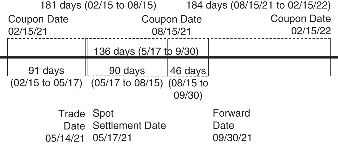
FIGURE 11.3 A Forward Contract on the US Treasury 1.125s of 02/15/2031.
- Note: no cash is generated or required on this date.
On August 15, 2021:
- Use the bond's coupon payment of
 to reduce the repo borrowing. More specifically, over the 90 days from May 17, 2021, to August 15, 2021, the repo loan balance grows to
  . Reducing this balance by the coupon payment leaves a balance of $95,231.70.
 - Note: no cash is generated or required on this date.
On September 30, 2021:
- Repay the repo loan, which, over the period August 15, 2021, to September 30, 2021, grows to
 .
. - Take back the $100,000 face amount of the 1.125s of 02/15/2031.
- Note: the bonds have effectively been purchased at a full price of 95.23353, which, subtracting the accrued interest of 0.14063 as of this date, equates to a flat price of 95.09290.
Algebraically, then, the full forward price of the 1.125s of 02/15/2031, 95.23353 can be written as,

Rearranging terms, and noting that the product of two interest rates is typically very small, gives the following approximation,

In words, in the case of an intermediate coupon, the full forward price approximately equals the future value to the forward date of the full spot price less the present value of the coupon payment. More generally, were there more than one intermediate coupon payment, the full forward price would approximately equal the future value of the full spot price minus the present values of all those intermediate coupons.
In both of these examples, forward bond prices are less than spot prices: for the 2.875s of 05/15/2028, the forward price of 109.72 is less than the spot price of 110.77, and for the 1.125s of 02/15/2031, the forward price of 95.09 is less than the spot price of 95.51. This relationship is typical and is commonly known as the forward drop.
To understand the intuition behind the forward drop, imagine that a trader has funds equal to the spot price and wants to own the bond as of the forward date. There are two possible strategies, which, by arbitrage, have to be equally appealing: i) use the funds to buy the bond spot and earn coupon interest to the forward date; and ii) buy the bond forward and invest the funds at the repo rate. If the coupon interest from strategy i) exceeds the repo interest from strategy ii), then the two strategies can be equally appealing only if the forward price is less than the spot price. But coupon interest on bonds typically does exceed the repo rate, because the term structure of interest rates is typically upward sloping. Hence, the forward price is usually less than the spot price, and there is usually a forward drop. Of course, if the repo rate exceeds the coupon rate, the argument reverses, and the forward price exceeds the spot price.
Consistent with this intuitive discussion, Appendix A11.1 shows that the forward drop of a bond approximately equals the difference between the interest earned on the bond and the cost of financing its purchase from the settlement date to the forward date. Following the terminology of Chapter 3, then, in which this difference is called cash carry, it follows that the forward drop approximately equals cash carry, or, in the jargon of forward and futures markets, simply “carry.” This point is illustrated here for these two examples. For the 2.875s of 05/15/2028, the difference between the spot and forward prices is ![]() , or about 1.06. At the same time, because the bond earns an actual/actual 2.875% semiannual coupon and finances at an actual/360 repo rate of 0.015%, the difference between the interest earned and the financing cost is about the same:
, or about 1.06. At the same time, because the bond earns an actual/actual 2.875% semiannual coupon and finances at an actual/360 repo rate of 0.015%, the difference between the interest earned and the financing cost is about the same: ![]() . For the 1.125s of 02/15/2031, the forward drop is
. For the 1.125s of 02/15/2031, the forward drop is ![]() , or 0.41. The difference between the coupon interest and financing cost is about the same:
, or 0.41. The difference between the coupon interest and financing cost is about the same: ![]() .
.
11.2 FORWARD BOND YIELD
As covered in Chapter 3, the yield to maturity of a bond is the single rate such that discounting the bond's cash flows at that rate, from spot settlement to maturity, gives the bond's (full) market price. The forward yield of a bond is defined analogously as the single rate such that discounting the bond's cash flows from forward settlement to maturity by that rate gives the bond's (full) forward price.
Figure 11.4 diagrams the relationship between the spot yield, the repo rate, and the forward yield, and Table 11.3 reports the spot and forward yields of the 2.875s of 05/15/2028 and the 1.125s of 02/15/2031, which are computed using Equation (A3.5) and the data given in the tables of previous section. As explained in that section, when the coupon rate exceeds the repo rate, market prices align such that investors are indifferent between i) buying a bond at its spot price, and ii) investing in repo to the forward date and buying the bond at its lower, forward price. Figure 11.4 and Table 11.3 make the same point in terms of yield: investors are indifferent between i) investing at the spot yield, and ii) investing in repo to the forward date and then at the higher, forward yield. Put another way, the spot yield is a complex weighted average of the relatively low repo rate and the relatively high forward yield, where the weights reflect the lengths of the relative holding periods, as indicated in Figure 11.4.

FIGURE 11.4 Spot Yields, Repo Rates, and Forward Yields.
TABLE 11.3 Spot and Forward Yields for the US Treasury 2.875s of 05/15/2028 and 1.125s of 02/15/2031, as of May 14, 2021, for Spot Settlement on May 17, 2021, and for Forward Settlement on September 30, 2021. The Repo Rate is 0.015%. Yields Are in Percent.
| Bond | Spot Yield | Forward Yield |
|---|---|---|
| 2.875s of 05/15/2028 | 1.260 | 1.337 |
| 1.125s of 02/15/2031 | 1.625 | 1.693 |
11.3 THE INTEREST RATE SENSITIVITY OF A FORWARD CONTRACT
What is the interest rate sensitivity or DV01 of a forward contract? With respect to DV01, and with reference to Figure 11.4, should DV01 be computed by shifting the spot yield, the forward yield, the repo rate, or some combination of the three? Table 11.4 shows the DV01s of the forward contracts in the examples of this chapter with respect to each of these rates. To compute the DV01 with respect to the spot yield, shift the spot yield down one basis point; calculate a new spot price; calculate a new forward price using the new spot price; and take the difference between the new and original forward prices. To compute the DV01 with respect to the forward yield, shift the forward yield down by one basis point; compute a new forward price using the new forward yield; and take the difference between the new and original forward prices. Finally, to compute the DV01 with respect to the repo rate, shift the repo rate down by one basis point; compute a new forward price using the new repo rate; and take the difference between the new and original forward prices.
TABLE 11.4 DV01 Metrics for the Forward Prices of the US Treasury 2.875s of 05/15/2028 and 1.125s of 02/15/2031, as of May 14, 2021, for Spot Settlement on May 17, 2021, and Forward Settlement on September 30, 2021. The Repo Rate Is 0.015%.
| 2.875s of 05/15/2028 | |
|---|---|
| Yield or Rate Shifted | DV01 |
| Spot Yield | 0.0708 |
| Forward Yield | 0.0666 |
| Repo Rate | −0.0042 |
| 1.125s of 02/15/2031 | |
| Yield or Rate Shifted | DV01 |
| Spot Yield | 0.0876 |
| Forward Yield | 0.0841 |
| Repo Rate | −0.0036 |
The DV01s of the two bonds with respect to the spot yields are consistent with their respective maturities of 7.0 and 9.75 years. The DV01s with respect to the repo rates are negative and small. They are negative, because – from the determination of the forward price in Equation (11.1), (11.2) or (11.3) – the forward price increases as the repo rate increases. And they are small, because the term of the underlying repo between the spot and forward settlement dates is 136 days, or a bit more than 0.37 years. Finally, the DV01s with respect to the forward yields can be understood as follows. A long forward position is equivalent to a long spot position and a short – borrowing cash – repo position. Therefore, the DV01 with respect to the forward yield is the sum of the (positive) DV01 with respect to the spot rate and the (negative) DV01 with respect to the repo rate.
Return now to the question of which of these DV01s should be used, keeping Figure 11.4 in mind. If the spot yield changes while the repo rate is constant, then a shift of the spot yield curve makes sense. If the spot yield and repo rate change together, by the same amount, then a shift of the forward yield makes sense. Taking this thinking a step further, some practitioners – recognizing the empirical regularity that longer‐term rates are more volatile than shorter‐term repo rates – assume that the repo rate changes by a fixed percentage of the spot yield change. At a percentage of 30%, for example, the DV01 of the forward contract is estimated as 30% times the (negative) DV01 with respect to the repo rate plus the (positive) DV01 with respect to the spot yield, which comes to 0.0695 for the forward on the 2.875s of 05/15/2028 and 0.0865 for the forward on the 1.125s of 02/15/2031. Varying this percentage from 0% to 100%, of course, gives estimates ranging from the DV01s given in Table 11.4 with respect to the spot yields to those with respect to the forward yields, respectively. The best approach, however, is to accept that the repo rate and long‐term yields can move independently and, therefore, to hedge in a two‐factor framework. Repo rate exposure should be hedged with other short‐term, fixed income instruments, and forward yield exposure should be hedged with longer‐term instruments.
11.4 MECHANICS OF US TREASURY NOTE AND BOND FUTURES
As mentioned at the start of the chapter, futures and forwards are essentially similar, in that they require the purchase or sale of bonds in the future, but futures embed various delivery options and require daily settlement. To present this material, the text focuses on the 10‐year US Treasury note futures contract maturing in September 2021, with the symbol “TYU1.” The “TY” is the code for the 10‐year contract; “U” is the code for September; and “1” denotes the last digit of the maturity year, here, 2021. The seller, or short, of one contract commits to sell or deliver $100,000 face amount of one of the deliverable Treasury notes listed in Table 11.5 at some time in the delivery month, in this case, September 2021. The buyer, or long, commits to buy or take delivery of $100,000 face amount of the Treasury note chosen by the seller at the time chosen by the seller. It is the seller, therefore, that has these two delivery options: the quality option, which is the option to choose which note to sell, or deliver, and the timing option, which is the option to choose when in the delivery month to sell. There are, in fact, two other delivery options, which are discussed later in the chapter: the end‐of‐month option, which arises because the last trading day of the futures contract (September 21, 2021, for TYU1) is seven business days before the last delivery date (September 30, 2021, for TYU1); and the wild‐card option, which arises because the futures settlement price on a given day is set hours before an intention to deliver has to be declared.
TABLE 11.5 The Deliverable Basket into TYU1.
| Conversion | ||
|---|---|---|
| Coupon | Maturity | Factor |
| 2.875 | 05/15/28 | 0.8338 |
| 2.875 | 08/15/28 | 0.8286 |
| 1.250 | 04/30/28 | 0.7474 |
| 1.250 | 03/31/28 | 0.7474 |
| 3.125 | 11/15/28 | 0.8376 |
| 2.625 | 02/15/29 | 0.8039 |
| 2.375 | 05/15/29 | 0.7836 |
| 1.625 | 08/15/29 | 0.7320 |
| 1.750 | 11/15/29 | 0.7331 |
| 1.500 | 02/15/30 | 0.7105 |
| 0.625 | 05/15/30 | 0.6462 |
| 0.625 | 08/15/30 | 0.6382 |
| 0.875 | 11/15/30 | 0.6476 |
| 1.125 | 02/15/31 | 0.6577 |
Once a seller has chosen which bond to deliver and when to deliver it, the price at which the bond is sold is the futures price at the time of delivery times the bond's conversion factor, as listed in Table 11.5. These conversion factors are fixed over the life of the futures contract. The reason for and computation of conversion factors is discussed next. For now, to focus on the mechanics, say that the futures price at expiration is 133.86. If the seller delivers the 2.875s of 05/15/2028, with a conversion factor of 0.8338, the price received is ![]() per 100 face amount. If the seller delivers the 1.125s of 02/15/2031, with a conversion factor of 0.6577, the price received is
per 100 face amount. If the seller delivers the 1.125s of 02/15/2031, with a conversion factor of 0.6577, the price received is ![]() . Also, as with any bond sale, the seller through a futures contract receives accrued interest as of delivery.
. Also, as with any bond sale, the seller through a futures contract receives accrued interest as of delivery.
TABLE 11.6 Settlement Prices of TYU1, from May 10, 2021, to May 28, 2021, and the Daily Settlement to a Long Position of One Contract. Changes Are in Ticks (32nds) and Daily Settlement Payments Are in Dollars.
| Daily | |||
|---|---|---|---|
| Date | Price | Change | Settlement |
| 05/10/2021 | 131–24 | ||
| 05/11/2021 | 131–19 | −5 | −156.25 |
| 05/12/2021 | 131–01 | −18 | −562.50 |
| 05/13/2021 | 131–10 | 9 | 281.25 |
| 05/14/2021 | 131–17+ | 7.5 | 234.38 |
| 05/17/2021 | 131–15+ | −2 | −62.50 |
| 05/18/2021 | 131–16+ | 1 | 31.25 |
| 05/19/2021 | 131–04 | −12.5 | −390.63 |
| 05/20/2021 | 131–19 | 15 | 468.75 |
| 05/21/2021 | 131−17+ | −1.5 | −46.88 |
| 05/24/2021 | 131–23+ | 6 | 187.50 |
| 05/25/2021 | 132–02+ | 11 | 343.75 |
| 05/26/2021 | 132–01 | −1.5 | −46.88 |
| 05/27/2021 | 131–25 | −8 | −250.00 |
| 05/28/2021 | 131–30 | 5 | 156.25 |
Futures contracts are subject to daily settlement. Throughout a trading day, market forces determine futures prices, and, at the end of each day, the exchange on which the futures trade determines a settlement price. For liquid contracts, like Treasury futures, the settlement price is usually the last traded price of the day. For some contracts, however, in exceptional circumstances, the exchange may substitute its judgment so that the daily settlement price reflects the end‐of‐day market level. In any case, Table 11.6 reports daily settlement prices for TYU1 from May 10, 2021, to May 28, 2021, per 100 face amount of the underlying bonds. Note that prices are reported in terms of “ticks” or 32nds, so that 131‐24 denotes a price of ![]() , or 131.75. Note too, that “+” means one half, so that 131‐17+ denotes a price of
, or 131.75. Note too, that “+” means one half, so that 131‐17+ denotes a price of ![]() , or 131.546875. The third column in the table shows the change in the daily settlement price, also measured in ticks, so that the settlement price fell by five ticks from May 10, 2021, to May 11, 2021.
, or 131.546875. The third column in the table shows the change in the daily settlement price, also measured in ticks, so that the settlement price fell by five ticks from May 10, 2021, to May 11, 2021.
The daily settlement feature of futures contracts requires that changes in the price of the contract be settled daily. These daily payments, for a long position of one contract in TYU1, are given in the last column of Table 11.6. From May 10, 2021, to May 11, 2021, for example, because the price of TYU1 falls by five ticks (per 100 face amount), the buyer loses value and must pay ![]() , which the exchange passes on to the seller. From May 12, 2021, to May 13, 2021, on the other hand, the settlement price increases by nine ticks, which means that the seller loses value and must pay
, which the exchange passes on to the seller. From May 12, 2021, to May 13, 2021, on the other hand, the settlement price increases by nine ticks, which means that the seller loses value and must pay ![]() , which the exchange passes on to the buyer. All futures market participants must post maintenance margin, usually in the form of a fixed number of dollars per contract, to protect the exchange against their defaulting on daily settlement payments.
, which the exchange passes on to the buyer. All futures market participants must post maintenance margin, usually in the form of a fixed number of dollars per contract, to protect the exchange against their defaulting on daily settlement payments.
With these mechanics explained, the differences between forward and futures contracts can be summarized as follows. First, forward contracts require the purchase and sale of a particular underlying security on a particular date, while futures contracts give the seller the right to choose the security (from a basket of deliverables) and to choose the date (in the delivery month). Second, the profit or loss from a forward contract is realized at the expiration of the contract, while the profit or loss from a futures contract is realized over time. Consider the futures prices in Table 11.6, which, over the period, increase a total of six ticks, from 131‐24 to 131‐30. Were this a forward contract, the buyer's profit would have increased by six ticks as of the expiration date, in this case, September 30, 2021. But because this is a futures contract with daily settlement, the buyer receives these six ticks as the price changes – some days receiving cash, some days paying cash, but cumulatively, from May 10, 2021, to May 28, 2021, receiving a total of six ticks. A related implication of this reasoning is that, as of May 28, 2021, the forward contract has value – it is a claim on six ticks at expiration – while the futures contract is worth zero – its value has already been fully paid. Put another way, after the settlement payment on May 28, 2021, the buyer of the futures contract on May 10, 2021, at 131‐24 has a zero‐value position, as does a new buyer of the contract on May 28, 2021, at 131‐30.3
11.5 PRICING AND HEDGING IMPLICATIONS OF DAILY SETTLEMENT
Daily settlement has implications for the pricing of futures relative to forwards and for hedging using futures rather than forwards. This section considers these two issues in turn.
Consider a forward contract and a futures contract on the same, single underlying bond, and assume for the moment that the initial forward and futures prices are the same. From the discussion in the previous section, changes in the prices of the forward contract are realized as profit and loss (P&L) cumulatively, as of expiration, while changes in the prices of the futures contract are realized as P&L daily. Which pattern of P&L realization is preferable to the buyer of a contract?
Because bond prices increase when interest rates fall, and vice versa, the buyer of a futures contract realizes profit early when rates fall, that is, when reinvestment opportunities are relatively poor. Similarly, the buyer realizes losses early when rates rise, that is, when the costs of financing those losses are relatively high. In other words, whether rates fall or rise, the early realization of P&L from a long bond futures position is undesirable. Hence, buyers are willing to pay less to purchase bonds through futures than through forwards, and, therefore, the futures price of a bond is less than its forward price. Appendix A11.3 formally proves this result.
In practice, the difference between futures and forward bond prices tends to be small. As evident from the previous paragraph and the appendix to this chapter, the magnitude of the difference depends on the covariance of the underlying bond price with the reinvestment or financing rate to contract expiration.4 But for note and bond futures, this covariance tends to be low: the time to contract expiration is typically short relative to the maturity of the underlying bonds; short‐term rates have relatively low volatility; and short‐term rates are imperfectly correlated with long‐term rates.
While the futures‐forward price difference tends to be small, traders normally do account for the difference in the timing of P&L cash flows when calculating hedge ratios. This is called tailing the hedge and is particularly common and useful for basis trades, which, as discussed presently, are trades of futures against synthetic bond forwards.
Consider a forward and futures contract on the same underlying security for delivery in ![]() days, when the term repo rate is
days, when the term repo rate is ![]() . Assume for simplicity that, over a given day, the forward and futures prices increase by the same amount,
. Assume for simplicity that, over a given day, the forward and futures prices increase by the same amount, ![]() . The futures contract, then, through daily settlement, pays
. The futures contract, then, through daily settlement, pays ![]() immediately to the long. The value to the long of the forward contract, by contrast, increases by
immediately to the long. The value to the long of the forward contract, by contrast, increases by ![]() as of the delivery date, or, in present value terms, by
as of the delivery date, or, in present value terms, by ![]() . Hence, for positive
. Hence, for positive ![]() , less than one futures contract hedges the change in value of one forward contract. More specifically, to hedge
, less than one futures contract hedges the change in value of one forward contract. More specifically, to hedge ![]() forward contracts with
forward contracts with ![]() futures contracts,
futures contracts,

where the difference between ![]() and
and ![]() is known as the tail of the hedge.
is known as the tail of the hedge.
This section closes with a comment on terminology. The terms “mark‐to‐market,” “variation margin,” and “daily settlement” are often used interchangeably, although, strictly speaking, they have distinct and different meanings. Mark‐to‐market is the process of adjusting security prices in an accounting framework to match market values. For example, securities in the trading book of a bank have to be marked‐to‐market when reported on its balance sheet, while securities designated as “held‐to‐maturity” can be reported at cost. The term mark‐to‐market, therefore, does not imply any exchange of cash. Variation margin refers to cash or securities that have to be posted as collateral to secure obligations under a contract. For example, as discussed in Chapter 10, borrowers of cash in the repo market have to make variation margin payments in the form of additional cash or securities as the value of their existing collateral declines. Counterparties posting collateral maintain ownership of that collateral, which means that i) interest is earned on the collateral either by being paid interest on cash collateral or by keeping interest earned on securities posted as collateral, and ii) collateral is returned when the associated contractual obligations have been fulfilled. Daily settlement, as described in this section, refers to the payment of gains or losses. These payments are irrevocable; that is, they do not earn interest and are never returned.5
11.6 COST OF DELIVERY AND THE FINAL SETTLEMENT PRICE
The cost of delivery measures how much it costs a short to fulfill the commitment to deliver a bond through a futures contract. Having decided to deliver bond ![]() , the short first has to buy the bond at its market price plus accrued interest and then deliver it through the futures contract for the futures price times the conversion factor plus accrued interest. Denoting the time‐
, the short first has to buy the bond at its market price plus accrued interest and then deliver it through the futures contract for the futures price times the conversion factor plus accrued interest. Denoting the time‐![]() flat price of bond
flat price of bond ![]() at time
at time ![]() by
by ![]() ; its accrued interest by
; its accrued interest by ![]() ; its conversion factor by
; its conversion factor by ![]() ; and the futures price by
; and the futures price by ![]() , the cost of delivery is,
, the cost of delivery is,
The short will choose which bond to deliver to minimize the cost of delivery. The bond that minimizes the cost of delivery is called the cheapest‐to‐deliver, or the CTD. Table 11.7 shows the price of TYU1, the prices of the bonds in its deliverable basket, and the costs of delivery for each of those bonds, as of the last trading date, September 21, 2021. For example, the cost of delivery of the 2.875s of 05/15/2028 is,
TABLE 11.7 Prices of TYU1 and Notes in Its Deliverable Basket as of the Last Trading Date, September 21, 2021.
| TYU1 | Price: | 133.85938 | |||
|---|---|---|---|---|---|
| Conversion | Cost of | Price / | |||
| Coupon | Maturity | Factor | Price | Delivery | Conv. Fac. |
| 2.875 | 05/15/2028 | 0.8338 | 111.61719 | 0.00524 | 133.86566 |
| 2.875 | 08/15/2028 | 0.8286 | 111.82813 | 0.91225 | 134.96032 |
| 1.250 | 04/30/2028 | 0.7474 | 101.14063 | 1.09413 | 135.32329 |
| 1.250 | 03/31/2028 | 0.7474 | 101.17969 | 1.13319 | 135.37555 |
| 3.125 | 11/15/2028 | 0.8376 | 113.76563 | 1.64501 | 135.82333 |
| 2.625 | 02/15/2029 | 0.8039 | 110.50000 | 2.89045 | 137.45491 |
| 2.375 | 05/15/2029 | 0.7836 | 108.82813 | 3.93592 | 138.88224 |
| 1.625 | 08/15/2029 | 0.7320 | 103.34375 | 5.35869 | 141.17999 |
| 1.750 | 11/15/2029 | 0.7331 | 104.33594 | 6.20363 | 142.32156 |
| 1.500 | 02/15/2030 | 0.7105 | 102.20313 | 7.09604 | 143.84676 |
| 0.625 | 05/15/2030 | 0.6462 | 94.89063 | 8.39070 | 146.84405 |
| 0.625 | 08/15/2030 | 0.6382 | 94.64844 | 9.21938 | 148.30529 |
| 0.875 | 11/15/2030 | 0.6476 | 96.57031 | 9.88298 | 149.12031 |
| 1.125 | 02/15/2031 | 0.6577 | 98.58594 | 10.54663 | 149.89499 |
Because this is the lowest cost of delivery in the table, these bonds are CTD into TYU1.
To focus on the quality option, assume for the moment that date ![]() is both the last trading date and the last delivery date. Arbitrage arguments can then be used to show that,
is both the last trading date and the last delivery date. Arbitrage arguments can then be used to show that,
and,
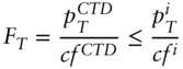
Equation (11.7) says that the cost of delivery of the CTD at expiration is zero. Equation (11.8) says that the futures price at expiration, that is, the last settlement price, equals the ratio of the price of the CTD bond to its conversion factor and that this ratio is less than or equal to the ratios of all other bond prices to their conversion factors. These theoretical predictions are extremely good approximations for TYU1 as of its last trading date, as can be seen from Table 11.7. The cost of delivery of the CTD is very close to zero; the ratio of its price to its conversion factor very nearly equals the futures price; and the ratio of all other bond prices to their CTDs are larger. This section concludes with the arbitrage proofs of Equations (11.7) and (11.8).
Say that (11.7) is not true, and that, instead, ![]() . In that case, an arbitrageur could buy the CTD, sell the futures, and deliver the CTD, earning a profit of,
. In that case, an arbitrageur could buy the CTD, sell the futures, and deliver the CTD, earning a profit of,
which is positive by the starting assumption that ![]() . Hence, ruling out market prices that admit riskless arbitrage opportunities rules out this assumed pricing relationship. Next, assume that
. Hence, ruling out market prices that admit riskless arbitrage opportunities rules out this assumed pricing relationship. Next, assume that ![]() . In this case, an arbitrageur could sell the CTD, buy the futures, and take delivery of the bond delivered by the short. If the short delivers the CTD, then the arbitrageur's profit is,
. In this case, an arbitrageur could sell the CTD, buy the futures, and take delivery of the bond delivered by the short. If the short delivers the CTD, then the arbitrageur's profit is,
which is positive by the starting assumption that ![]() . If the short delivers some other bond
. If the short delivers some other bond ![]() , the trader buys back the CTD just sold and sells bond
, the trader buys back the CTD just sold and sells bond ![]() instead, for a total profit of,
instead, for a total profit of,
where the first inequality follows from the definition of the CTD – the cost of delivering any bond other than the CTD is at least as great as the cost of delivering the CTD – and the second inequality follows from the starting assumption that ![]() . Hence, the arbitrageur's profit is even greater if the short (suboptimally) delivers a bond other than the CTD. But if the arbitrageur's profit is positive for whatever bond the short delivers, then the assumption
. Hence, the arbitrageur's profit is even greater if the short (suboptimally) delivers a bond other than the CTD. But if the arbitrageur's profit is positive for whatever bond the short delivers, then the assumption ![]() is ruled out as admitting riskless arbitrage opportunities. Finally, ruling out both
is ruled out as admitting riskless arbitrage opportunities. Finally, ruling out both ![]() and
and ![]() proves the equality in (11.8) and (11.7). The inequality of (11.8) follows from combining (11.7) with the condition that the CTD has the lowest cost of delivery,
proves the equality in (11.8) and (11.7). The inequality of (11.8) follows from combining (11.7) with the condition that the CTD has the lowest cost of delivery,

11.7 MOTIVATIONS FOR A DELIVERY BASKET AND CONVERSION FACTORS
Historically, the design of bond futures contracts purposely avoided a single underlying security. One reason is to ensure that the liquidity of the futures contract does not depend on the liquidity of a single, underlying bond, which might lose its liquidity for idiosyncratic reasons, for example, through being accumulated by a few large, buy‐and‐hold investors. A second reason is to avoid losing liquidity to the threat of a squeeze. A trader squeezes a contract by simultaneously buying many contracts and a large fraction of the deliverable bond, hoping to sell the position at a profit when traders who had sold contracts – but cannot find bonds to deliver – have to pay up to buy the deliverable bond or to buy back the contracts from the perpetrator of the squeeze. The threat of a squeeze, which makes shorts hesitant to take positions, can prevent a contract from attracting volume and liquidity.
A deliverable basket avoids the problems of a single deliverable so long as some bonds can be delivered at a cost not too much greater than the cost of delivering the CTD. In Table 11.7, delivering the 2.875s of 08/15/2028 is about 91 cents per 100 face amount more costly than delivering the CTD, and the 1.250s of 04/30/2028 are about 18 cents more costly than that. The relatively inexpensive substitutability of these near CTD bonds limits the profit potential of a squeeze. After going to all the trouble, expense, and risk of buying many contracts and a large fraction of the outstanding CTD bonds, shorts would refuse to pay a premium of more than about 100 cents per 100 face amount of the CTD, because the two bonds just mentioned can be delivered instead.
Limiting the costs of delivery of at least some bonds other than the CTD is accomplished by conversion factors. In Table 11.7, the costs of delivering the five bonds with the lowest costs of delivery range from about zero to 1.65. This range would be a lot wider, however, if there were no conversion factors, or, more precisely, if all conversion factors were implicitly equal to 1.0. In that case, sellers would receive the futures price for delivering any bond; would choose to deliver the bond with the lowest price; and, therefore, the market futures price would equal that lowest price. Referring back to Table 11.7, the CTD bond would be the 0.625s of 08/15/2030, which has the lowest price of about 94.65, and the futures price would be 94.65. Furthermore, the five lowest bond prices, which range from that 94.65 to the 101.14 price of the 1.25s of 04/30/2028, would imply costs of delivery that range from zero to ![]() or 6.49, which is a lot wider than the range with the conversion factors of TYU1.
or 6.49, which is a lot wider than the range with the conversion factors of TYU1.
Conversion factors reduce the difference in delivery costs by adjusting delivery prices for the differences across bond coupon rates. Given the limited maturity range of bonds deliverable into TYU1, a major determinant of the price differences across bonds is coupon rate. The most expensive bond in Table 11.7 is the bond with the highest coupon, the 3.125s of 11/15/2028, with a price of 113.77. The least expensive deliverable bond is one of the bonds with the lowest coupon, the 0.625s of 8/15/2030, with a price of 94.65. Conversion factors essentially recognize that sellers are delivering expensive, high‐coupon bonds rather than inexpensive, low‐coupon bonds. For example, the conversion factor of the 3.125s of 11/15/2028 is 0.8376, while the conversion factor of the 0.625s of 08/15/2030 is 0.6382. A glance at the table reveals that bonds with higher coupons tend to have higher conversion factors.
Conversion factors are computed by the exchange and are easily available. The basic idea can be explained most simply, however, with the following approximation: the conversion factor of a bond equals its price, per dollar face amount, at a yield equal to the notional coupon rate, for settlement on the last delivery date. At present, the notional coupon for US Treasury futures is 6%. Therefore, to take one example, the conversion factor of the 1.25s of 03/13/2028 deliverable into TYU1 is approximated using the price‐yield Equation (3.8) for a face amount of one dollar, at a yield of 6%, and for settlement on 09/30/2021, which leaves 13 remaining coupon payments,6

This calculation rule clearly assigns higher conversion factors to higher coupon bonds. But the justification for the rule is stronger than that. Assume that the term structure of yields is actually flat at 6%. In that case, the conversion factor of each bond equals the market price of one dollar face amount of the bond, and the ratio of the market price (per 100 face amount) to the conversion factor equals 100 for every bond. Furthermore, by the arguments of the previous section, the futures price is 100; the cost of delivery of each bond is zero; and all bonds are jointly CTD. In short, if market yields are flat at the notional coupon, conversion factors make every bond as attractive to deliver as any other, thus lessening the dependence of the contract's liquidity on the liquidity of any one bond and also reducing, if not eliminating, the potential profits of a squeeze.
Because the yield curve is not flat at the notional coupon rate, however, conversion factors limit but do not eliminate differences in the costs of delivery across bonds, as evident from Table 11.7. The resulting emergence of a unique CTD is the subject of the next section.
11.8 THE QUALITY OPTION AT EXPIRATION
To illustrate how the quality option works at expiration of the futures contract, assume for the moment that the 2.875s of 05/15/2028 and the 1.125s of 02/15/2013 are the only deliverable bonds into TYU1. Figure 11.5 graphs the ratio of price to conversion factor against yield for these two bonds as of the last trading date, September 21, 2021. The figure assumes that the term structure of yields is flat, that is, that the two bonds have the same yield at the indicated level. At a yield of 6%, the price‐conversion factor ratio of each of the bonds is about 100: as explained in the previous section, the conversion factor is approximately equal to the price of the bond (per dollar face amount) at a yield of the notional coupon rate – here 6% – as of the last delivery date (which is only a few days different from the last trading date). Hence, the ratio of each bond's price (per 100 face amount) to its conversion factor is about 100. Furthermore, the futures price is 100, the costs of delivering either bond is zero, and the two bonds are jointly CTD.
As rates move away from 6%, however, the costs of delivering the two bonds diverge. Conversion factors are fixed to equate the price‐conversion factor ratio of the two bonds at a yield of 6%. But as yields fall below 6%, the price and price‐conversion factor ratio of the shorter‐maturity and shorter‐duration 2.875s of 05/15/2028 increase more slowly than the price and price‐conversion factor ratio of the longer‐maturity and longer‐duration 1.125s of 02/15/2031. Therefore, for yields below 6%, the 2.875s of 05/15/2028 are CTD. On the other hand, as yields rise above 6%, the price‐conversion factor ratio of the longer‐duration 1.125s of 02/15/2031 falls more quickly, and that bond is CTD.
The futures price equals the lowest price‐conversion factor ratio across deliverable bonds. Graphically, in the present example, the price of TYU1 is the minimum or lower envelope of the two price‐conversion factor curves, depicted in Figure 11.5 by a semi‐transparent, gray band. At expiration, the futures price tracks the price of the low‐duration bond when rates are low and the price of the high‐duration bond when rates are high.
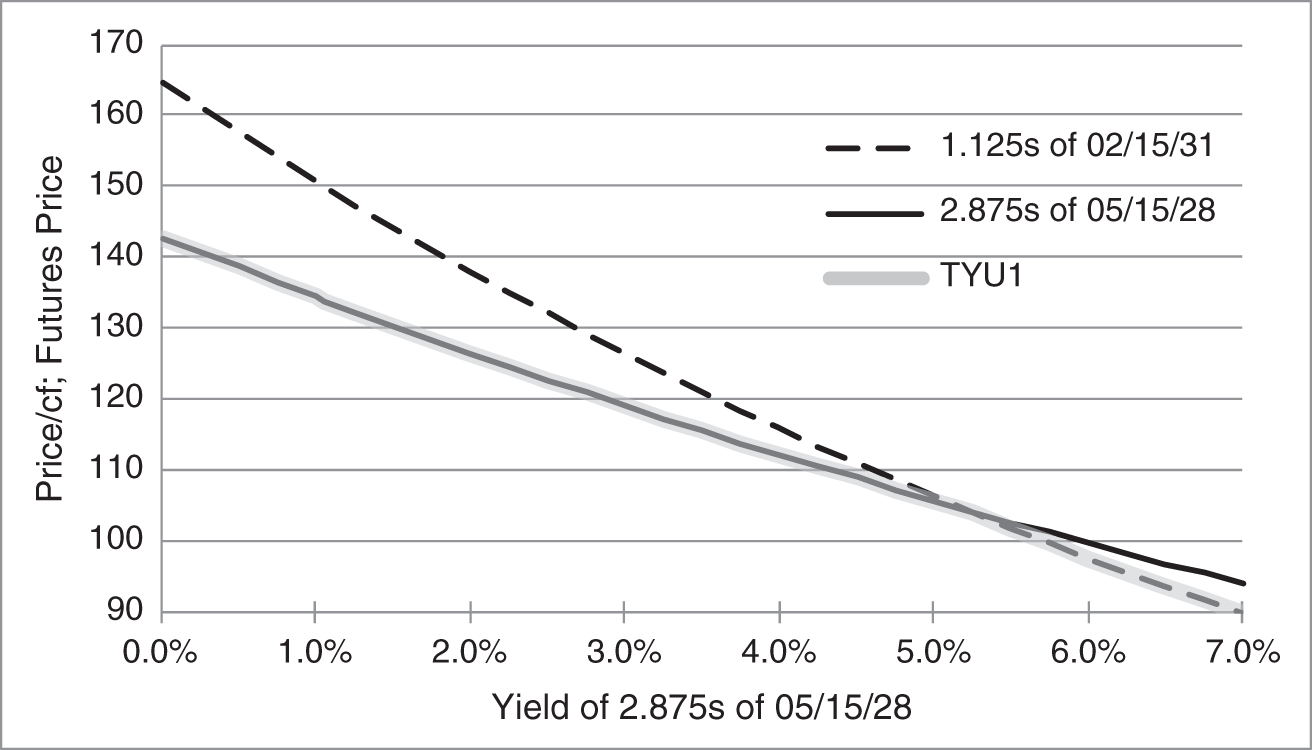
FIGURE 11.5 Quality Option for TYU1 with a Flat Term Structure of Yields, as of the Last Trading Date.
Figure 11.5 is stylized in two ways. First, because there are many deliverable bonds, several distinct ranges of yield at expiration might each determine a different CTD. Along the lines of the discussion here, however, the deliverable bond with the shortest duration is typically CTD at the lowest range of yields; deliverable bonds with intermediate durations might be CTD at intermediate ranges of yield; and the deliverable bond with the longest duration is typically CTD at the highest range of yields.
The second way Figure 11.5 is stylized is in assuming that the yields of the two bonds are equal and move up or down in parallel. In reality, the term structure of interest rates and individual bond yields can move in many ways that affect the determination of the CTD. Most generally, a bond is more likely to be CTD after any change that cheapens it relative to other bonds in the deliverable basket. If the term structure flattens, shorter‐term bonds are more likely to be CTD. If the term structure steepens, longer‐term bonds are more likely to be CTD. And if the yield of any bond increases idiosyncratically relative to yields of other deliverable bonds, that bond is more likely to be CTD.
11.9 GROSS AND NET BASIS AND BASIS TRADES
The gross basis and net basis of a deliverable bond measure the difference between the price of that bond and the relevant futures contract. The gross basis of a bond is convenient for quoting the prices of packages, that is, the terms at which traders can buy a futures contract and short a deliverable bond, or vice versa. The net basis is a measure of a bond's proximity to being CTD, and changes in a bond's net basis give the P&L of a basis trade. Lastly, a basis trade is the purchase of a futures contract and the forward sale of a deliverable bond, or vice versa, usually to take advantage of a perceived mispricing of futures relative to the deliverable bonds.
Let ![]() denote the spot price of bond
denote the spot price of bond ![]() at time
at time ![]() ;
; ![]() its forward price at time
its forward price at time ![]() to the last delivery date,
to the last delivery date, ![]() ; and
; and ![]() its conversion factor. Let
its conversion factor. Let ![]() be the futures price at time
be the futures price at time ![]() . Then, the gross basis and net basis of bond
. Then, the gross basis and net basis of bond ![]() at time
at time ![]() ,
, ![]() and
and ![]() , respectively, are defined as,
, respectively, are defined as,
Table 11.8 gives the futures price and the spot and forward prices of each bond deliverable into TYU1, along with its gross basis, carry, and net basis.7 For example, the gross basis of the 2 7/8s of 05/15/2028 is,

which is 32 times 1.0896, or 34.9 ticks. The net basis of that bond is,
or 1.1 ticks.
As defined, the difference between the gross basis and the net basis of a bond equals the difference between its spot and forward prices, which, as shown earlier, equals its carry. This explains the terminology: the net basis is the gross basis net of carry. Continuing with the example, the carry of the 2.875s of 05/15/2028 – from May 17, 2021 (spot settlement), to September 30, 2021 (last delivery date) – is calculated earlier in the chapter as 1.057 or 33.8 ticks. Hence, the bond's gross basis of 34.9 ticks minus its carry of 33.8 ticks equals its net basis of 1.1 ticks. It similarly follows from the definitions that, as of contract expiration – when the forward price for settlement on contract expiration is the same as its spot price at contract expiration – gross and net basis are equal to each other and to the bond's cost of delivery, as defined in Equation (11.5). Furthermore, because the cost of delivery at expiration of the CTD is zero, its gross and net basis at expiration are also zero.
TABLE 11.8 Gross and Net Basis of Deliverable Notes into TYU1 as of May 14, 2021. Repo Rate from Spot Settlement to the Last Delivery Date is 0.015%. Gross Basis, Carry, and Net Basis Are in Ticks (32nds).
| TYU1 | Price: | 131‐17+ | |||||
|---|---|---|---|---|---|---|---|
| Conv. | Spot | Gross | Fwd | Net | |||
| Coupon | Maturity | Factor | Price | Basis | Price | Carry | Basis |
| 2.875 | 05/15/2028 | 0.8338 | 110‐24 3/4 | 34.9 | 109.7172 | 33.8 | 1.1 |
| 2.875 | 08/15/2028 | 0.8286 | 110‐27 | 59.0 | 109.7759 | 34.2 | 24.8 |
| 1.250 | 04/30/2028 | 0.7474 | 99‐26 1/4 | 48.1 | 99.3615 | 14.7 | 33.4 |
| 1.250 | 03/31/2028 | 0.7474 | 99‐29 1/4 | 51.1 | 99.4578 | 14.6 | 36.5 |
| 3.125 | 11/15/2028 | 0.8376 | 112‐22 1/4 | 80.4 | 111.5468 | 36.8 | 43.6 |
| 2.625 | 02/15/2029 | 0.8039 | 109‐03+ | 107.5 | 108.1348 | 31.2 | 76.3 |
| 2.375 | 05/15/2029 | 0.7836 | 107‐07 1/4 | 132.7 | 106.3549 | 27.9 | 104.8 |
| 1.625 | 08/15/2029 | 0.7320 | 101‐13+ | 164.1 | 100.8205 | 19.2 | 144.9 |
| 1.750 | 11/15/2029 | 0.7331 | 102‐07+ | 185.5 | 101.5934 | 20.5 | 165.0 |
| 1.500 | 02/15/2030 | 0.7105 | 99‐27 1/4 | 204.4 | 99.2968 | 17.8 | 186.6 |
| 0.625 | 05/15/2030 | 0.6462 | 92‐05 1/4 | 229.1 | 91.9383 | 7.2 | 221.8 |
| 0.625 | 08/15/2030 | 0.6382 | 91‐24 3/4 | 250.2 | 91.5451 | 7.3 | 242.9 |
| 0.875 | 11/15/2030 | 0.6476 | 93‐20 1/4 | 270.2 | 93.3147 | 10.2 | 260.0 |
| 1.125 | 02/15/2031 | 0.6577 | 95‐16 1/4 | 287.7 | 95.0929 | 13.3 | 274.4 |
Gross and net basis are particularly useful in the context of basis trades. To buy or be long a bond's basis, a trader buys a bond forward to contract expiration and sells a conversion‐factor weighted number of futures contracts. To sell or be short a bond's basis, a trader sells a bond forward to contract expiration and buys a conversion‐factor weighted number of futures contracts. In the US Treasury market, where spot and repo markets are much more liquid than forward markets, forward purchases and sales of bonds are typically synthetic, as described earlier in the chapter. A conversion‐factor weighted number of contracts is the number of contracts corresponding to the face amount of the bonds times the bond's conversion factor. For example, a trader buying $100 million of the 2.875s of 05/15/2028 TYU1 basis buys $100 million face amount of the bonds forward and sells 0.8338 times $100 million divided by $100,000, or about 834 contracts.
Gross basis is often used to quote a package trade of bonds against futures. A trader might put in an order, for example, to buy $100 million face amount of the 2.875s of 08/15/2028 and sell 834 TYU1 contracts at a gross basis of 34.9 ticks or less. If prices subsequently line up such that the bond price minus 0.8338 times the futures price is less than or equal to 34.9 ticks, the trade is executed. The trader then sells the repo to TYU1's expiration date to complete the basis trade.
Abstracting for a moment from interest on daily settlement payments, the P&L of a long basis position is the sum of the profit or loss from the forward bond position and from the futures position. Algebraically, with ![]() face amount of bond
face amount of bond ![]() and a trade from time
and a trade from time ![]() to time
to time ![]() , the P&L is,
, the P&L is,
But, from the definition of the net basis in Equation (11.15), (11.18) can be rewritten as,
In words, the P&L of a long basis trade is the face amount of bonds times the change in the bond's net basis. The P&L of a short basis trade is the negative of that. Consider, then, a trader who is sure that a particular bond will be CTD at expiration but sees that the net basis of the bond is trading at five ticks. This trader might very well sell the basis in the hope of making five ticks: if the bond does turn out to be CTD, its net basis will be zero at expiration, and the trader's profit will be the difference between the initial net basis of five ticks and the final net basis of zero ticks. Along these lines, therefore, the net basis of a bond is an indicator of a bond's becoming CTD. With respect to TYU1 as of May 14, 2021, the net bases in Table 11.8 strongly indicate that the 2.875s of 05/15/2028 will be CTD at expiration. Price are such that traders cannot make much money by betting that the 2.875s of 05/15/2028 will be CTD, that is, by selling its basis at only 1.1 ticks. But they can make a lot of money by taking a contrarian view that turns out to be right, for example, by selling the 2.875s of 08/15/2028 basis at 24.8 ticks in the hope that this bond will turn out to be CTD.
The interpretation of net basis in the previous paragraph implicitly assumes that the futures price is fair, or valued correctly, relative to the prices of the underlying bonds and their volatility. In terms of TYU1 as of May 14, 2021, assuming that the futures price is fair is equivalent to saying that the net basis of the 2.875s of 05/15/2028 is 1.1 ticks – rather than zero – because there is still some chance that another bond will turn out to be CTD at delivery. But some trader might believe that bond price volatility from May 14, 2021, to September 30, 2021, is much too small for a change in the CTD to be possible. From that trader's perspective, the market's net basis of the 2.875s of 05/15/2028, at 1.1 ticks, is too high; that is, the price of the 2.875s of 05/15/2028 is too high relative to the futures price. In this sense, net basis can be an indicator of relative value.
This section closes with two details about gross and net basis and basis trades. First, Equations (11.18) and (11.19) are not completely accurate expressions of the P&L of basis trades as described, because interest is paid or earned on daily settlements of the futures contract. As mentioned earlier, however, tailing the hedge does account for daily settlements. Therefore, these P&L equations are accurate representations of P&L for basis trades with a tail hedge, that is, not with a conversion‐factor weighted number of futures contracts, but with a conversion‐factor weighted and tailed number of futures contracts. Second, some traders, instead of selling or buying the repo to the term of the futures contract, sell or buy overnight repo. These traders are not really buying or selling the bonds forward against their futures positions, and the resulting P&L is not equal to that given in Equations (11.18) and (11.19). The case study at the end of this chapter discusses the risks of a “basis” trade with overnight rather than term repo.
11.10 IMPLIED REPO RATES
Table 11.1 and Equation (11.1) compute the forward price of the 2.875s of 05/15/2028 given its price for spot settlement and its term repo rate from spot to forward settlement. The same relative pricing formula can be applied, of course, to compute the repo rate given a bond's forward and spot prices. Under the assumption that a particular bond will be CTD into a futures contract, a repo rate computed in this way is called that bond's implied repo rate.
To illustrate, consider, once again, the 2.875s of 05/15/2028 and the data in Table 11.8. If that bond will be CTD with certainty, the ratio of its forward price to its conversion factor should equal the futures price; that is, its forward price should equal ![]() , or 109.68379.8 Then, following the logic of Equation (11.1), the relationship between the bond's spot and forward prices and the repo rate,
, or 109.68379.8 Then, following the logic of Equation (11.1), the relationship between the bond's spot and forward prices and the repo rate, ![]() , is,
, is,

which gives an implied repo rate of ![]() .
.
It is evident from Equations (11.1) and (11.20) that a lower repo rate generates a lower forward price. Therefore, if a bond will be CTD with certainty, and if its implied repo rate is less than its actual repo rate, then the futures price is cheap relative to the bond's spot price. Similarly, if a bond will be CTD with certainty, and if the implied repo rate of a bond is greater than its actual repo rate, then the futures price is rich relative to the bond's spot price. In the example, under the assumption that the 2.875s of 05/15/2028 will be CTD, an implied repo rate of ![]() 0.065% and an actual repo rate of 0.015% imply that TYU1 is cheap relative to the CTD's spot price.
0.065% and an actual repo rate of 0.015% imply that TYU1 is cheap relative to the CTD's spot price.
Another way to think about implied repo is as the rate earned by buying a bond spot and selling it through the futures contract. Rewriting Equation (11.1), with a spot price of 110.77344 and a forward price of 109.71721, the return from buying spot and selling forward is just the repo rate,

Similarly, the return from buying spot and selling forward – this time with a forward price implied by the futures price of 109.68379 – is ![]() 0.065%. From this perspective as well, then, TYU1 is too low relative to the spot price of the 2.875s of 05/15/2028, so long as that bond is CTD. Implied repo as a measure of relative value will be revisited in the case study at the end of the chapter.
0.065%. From this perspective as well, then, TYU1 is too low relative to the spot price of the 2.875s of 05/15/2028, so long as that bond is CTD. Implied repo as a measure of relative value will be revisited in the case study at the end of the chapter.
11.11 FUTURES PRICE AND THE QUALITY OPTION BEFORE EXPIRATION
It is shown earlier, and illustrated in Table 11.7, that the futures price at expiration is the minimum ratio of price to conversion factor across deliverable bonds. This section analyzes the futures price before expiration. The basic idea is as follows. If the CTD were known with certainty, then (abstracting from the futures‐forward difference) the futures price would equal the forward price of the CTD divided by its conversion factor. But because the CTD is not known with certainty, and because the seller of the futures contract has the option to choose which bond to deliver, the futures price is reduced by the value of that delivery option.
To illustrate this idea graphically, Figure 11.6 shows a yield‐price curve for TYU1, as of May 14, 2021, along with the ratios of forward prices to conversion factors for two deliverable bonds – the shortest‐duration bond in the basket, the 2.875s of 05/15/2028, and the longest‐duration bond in the basket, the 1.125s of 02/15/2031. The horizontal axis gives the assumed yield of the 2.875s of 05/15/2028 as of May 14, 2021, which for graphical clarity, is limited to the range of 4.00% to 5.50%. The yield of the 1.125s of 02/15/2031 and the repo rate are assumed to be at fixed spreads to the yield of the 2.875s of 05/15/2028.9 The futures price corresponding to each yield of the 2.875s of 05/15/2028 is calculated using a very simple model, which assumes that i) changes in the yield of the 2.875s of 05/15/2028 from its starting value along the horizontal axis to the expiration date, September 30, 2021, are normally distributed with a volatility of 100 basis points per year; ii) spreads of the yield of the 1.125s of 02/15/2031 and the repo rate to the yield of the 2.875s of 05/15/2028 are fixed; and iii) delivery occurs on September 30, 2021; that is, only the quality option is considered. The appendix to this chapter describes the pricing of futures in a term structure model in more detail.

FIGURE 11.6 TYU1 Price with Two Deliverable Bonds, as of May 14, 2021. Yields Are Assumed to Move in Parallel with a Volatility of 100 Basis Points per Year.
There are only four and a half months from the pricing date of the figure, May 14, 2021, to the last delivery date, September 30, 2021. Therefore, when yields are very low on May 14, 2021, it is extremely likely that the relatively low‐duration 2.875s of 05/15/2028 will be CTD at expiration. Or, put differently, it is extremely unlikely that rates will rise enough for the relatively high‐duration 1.125s of 02/15/2031 to become CTD. Recognizing this, the market assumes that the 2.875s of 05/15/2028 will be delivered and sets that bond's net basis very close to zero, or, equivalently, sets the futures price very near the ratio of that bond's forward price to its conversion factor. This can be seen in Figure 11.6: for low rates, the semi‐transparent, gray band representing the futures price converges to the forward price‐conversion factor ratio of the 2.875s of 05/15/2028. Analogously, when rates are very high on May 14, 2021, it is extremely likely that the relatively high‐duration 1.125s of 02/15/2031 will be CTD; its net basis is near zero; and the futures price converges to the ratio of its forward price to its conversion factor.
For intermediate rates shown in the figure, the futures price is less than the forward price‐conversion factor ratio of both bonds. Buyers will not price the futures under the assumption that the 2.875s of 05/15/2028 are delivered with certainty, because the sellers – who minimize the value of the futures – will switch from delivering the 2.875s of 05/15/2028 to delivering the 1.125s of 02/15/2031 exactly in those scenarios that hurt the buyers. Hence, the futures price must be lower than it would be under the assumption that the 2.875s of 05/15/2028 will be delivered with certainty. By the same logic, the futures price must be lower than it would be under the assumption that the 1.125s of 02/15/2031 will be delivered with certainty. In fact, the distance between either bond curve and the futures price curve at a given yield represents the value of the seller's option to switch from delivering one bond to delivering the other. That value is low when rates are very high or very low, because one bond or the other is almost certain to be delivered. Furthermore, if the assumed volatility of yields were higher, so that yields are more likely to move far from their levels as of the pricing date, the option to switch would increase in value, and the futures curve would be even more below the bond curves.
Figure 11.7 illustrates the value of the quality option as of May 14, 2021, for yields as of that pricing date ranging from 0% to 7%, in terms of the net basis of three bonds: the low‐ and high‐duration bonds described earlier, and an intermediate‐duration bond in the basket, the 3.125s of 11/15/2028. These curves are computed using the same model as in Figure 11.6.

FIGURE 11.7 Net Basis of Three Bonds Deliverable into TYU1, as of May 14, 2021. Yields Are Assumed to Move in Parallel with a Volatility of 100 Basis Points per Year.
The net basis of the low‐duration bond, the 2.875s of 05/15/2028, is near zero for low yields, because at those levels of yields on May 14, 2021, it will almost certainly be the CTD at expiration. As rates increase, however, because it becomes more likely that the 1.125s of 02/15/2031 will be CTD, the net basis of the 2.875s of 05/15/2028 increases. Put another way, this net basis increases because the value of the seller's option to switch away from delivering the 2.875s of 05/15/2028 increases. In contrast, the net basis of the high‐duration bond, the 1.125s of 02/15/2031, is near zero for high yields, when it will almost certainly be CTD at expiration. As yields fall, however, its becoming CTD is less of a certainty, and its net basis increases.
The net basis of the 3.125s of 11/15/2028 is never close to zero, because it is never likely to become CTD. While the set of deliverables can, in general, lead to ranges of yields in which intermediate‐duration bonds are CTD at expiration, for TYU1 as of May 14, 2021, and under the assumption of parallel shifts, the CTD at expiration is heavily likely to be either the lowest‐duration bond, the 2.875s of 05/15/2028, or the highest‐duration bond, the 1.125s of 02/15/2031. Nevertheless, at a yield level of about 4% as of the pricing date, the 3.125s of 11/15/2028 are as close as they ever are to being CTD at expiration, and their net basis falls to a minimum of about nine ticks. For lower yields and for higher yields, the 3.125s of 11/15/2028 are even less likely to wind up as the CTD, as their net basis increases accordingly.
The net basis graphs in Figure 11.7, as manifestations of the quality option, can be described more directly in terms of option terminology. The net basis of the low‐duration bond resembles a call option on rates, or, equivalently, a put option on bond prices; the net basis of the intermediate‐duration bond resembles a straddle on rates and bond prices; and the net basis of the high‐duration bond resembles a put on rates or a call option on bond prices.
The price‐yield curve of TYU1 in Figure 11.6, which incorporates the seller's quality option, can be used to derive the DV01 of the futures contract, as defined in Chapter 4: the change in price for a one‐basis‐point decline in rates. The DV01s of the 2.875s of 05/15/2028 and 1.125s of 02/15/2031, divided by their respective conversion factors, along with the DV01 of TYU1, are graphed Figure 11.8. As expected, the DV01 of the shorter‐maturity bond is relatively low and flat, with the flatness indicative of its lower convexity, while the DV01 of the longer‐maturity bond is relatively high and steep, with the steepness indicative of its higher convexity. The futures price‐yield relationship, however, differs markedly from that of a coupon bond. At low yields as of the pricing date, the futures DV01 resembles the DV01 divided by conversion factor of the bond most likely to be CTD at expiration, namely the shorter‐maturity 2.875s of 05/15/2028. Analogously, at high yields as of the pricing date, the futures DV01 resembles that of the 1.125s of 02/15/2031 divided by its conversion factor. At intermediate yields, the DV01 of the futures contract gradually changes from following that of the short‐maturity bond to following that of the high‐maturity bond. Therefore, its DV01 increases as yields increase, which means that TYU1 is negatively convex over that region of intermediate yields. This negative convexity is also visible, of course, in the shape of the TYU1's price‐yield curve in Figure 11.6.

FIGURE 11.8 DV01 of TYU1 and the DV01s of Two Deliverable Bonds Divided by Their Conversion Factors, as of May 14, 2021. Yields Are Assumed to Move in Parallel with a Volatility of 100 Basis Points per Year.
As of May 14, 2021, the yield of the 2.875s of 05/15/2028 was, in fact, 1.26%. In this low‐rate environment, it is clear from Figures 11.6, 11.7, and 11.8 that the 2.875s of 05/15/2028 are solidly CTD: the quality option is worth very little; the futures contract – apart from daily settlement considerations – is essentially a forward contract on the 2.875s of 05/15/2028; and the futures price is approximately equal to the forward price of that bond divided by its conversion factor. These conclusions are all evident in Table 11.8, which shows that, as of May 14, 2021, the net basis of the 2.875s of 05/15/2028 is 1.1 ticks, and, therefore, the futures price of 131‐17+, or about 131.55, is very close to the ratio of that bond's forward price to its conversion factor, ![]() , or 131.59.
, or 131.59.
These observations raise the question of why the notional coupon of the contract has not been lowered from 6%. As discussed already, when the yield curve is flat at 6%, conversion factors make all bonds equally deliverable, which, in turn, lowers liquidity dependence on a single CTD and reduces the profitability of a squeeze. That the term structure is not flat, and that bonds sell at idiosyncratically variable yields means that conversion factors are not perfect with respect to these objectives, but setting the notional coupon close to prevailing market levels does significantly reduce differences in deliverability across bonds. Again, then, why has the notional coupon not been set closer to market levels, that is, at somewhere between 1% and 2%? After all, the current notional coupon of 6% was reduced from its previous level of 8% in response to lower market rates.
A likely answer has two parts. First, with the increase of volumes and liquidity of both Treasury bonds and Treasury futures, the risks of a fall in liquidity or a squeeze have diminished. Second, as evident from the discussions in this chapter, valuing the quality option is quite complex. Overall, market participants – apart from basis arbitrage traders – seem to prefer a simpler contract, one effectively without delivery options, which is, therefore, easier to price and hedge.
11.12 THE TIMING, END‐OF‐MONTH, AND WILD‐CARD OPTIONS
As mentioned earlier, the timing option allows the seller to deliver at any time during the delivery month. For TYU1, for example, delivery is allowed at any date between September 1, 2021, and September 30, 2021. To understand whether sellers should deliver late or early, consider a trader who is long the bond and short the futures. Delivering late earns carry on the bond coupon until delivery and preserves full use of the quality option. Delivering early and investing the proceeds at the repo rate gives up carry on the bond and any remaining value of the quality option. Therefore, so long as carry is positive, it is optimal to delay delivery. Because coupon rates are typically greater than repo rates, carry is typically positive and late delivery typically optimal. If carry is negative, however, which is most likely for shorter‐maturity contracts when the short end of the term structure is downward sloping, then the carry advantage of early delivery has to be weighed against the lost option value.
Before analyzing the end‐of‐month option, the discussion turns to the fact that the last trading date of Treasury note and bond futures is seven business days before the last delivery date. For TYU1, for example, the last trading date is September 21, 2021, while the last delivery date is September 30, 2021. This feature of the contract requires an adjustment to futures hedges just after the last trading date. To see this, consider a basis position on the last trading date. For simplicity, continuing with TYU1, assume that the 2.875 of 05/15/2028 is almost certain to be CTD, and that, with the delivery date so near, its forward and spot prices are approximately equal. Now consider a $1 billion long basis position in that CTD, which is long $1 billion face amount of the bond and short 8,338 TYU1 contracts. This position is hedged because the futures price equals the CTD bond price divided by its conversion factor, 0.8338. If, for example, the price of the bond falls from 111.62 to 110.62, causing a loss on the (long) bond side of the trade of $1 billion × (111.62% − 110.62%), or $10 million, the futures price falls 8,338 × $100,000 × (111.62%/0.8338 − 110.62%/0.8338), for a gain on the (short) futures side of the trade of an offsetting $10 million. After the last trading date, however, the futures price is frozen at its last settlement price, say of ![]() , or 133.8690, and the delivery price of the CTD is frozen at
, or 133.8690, and the delivery price of the CTD is frozen at ![]() . If the CTD now falls in price to 110.62, the value of the long bond position again falls by $10 million, but the short futures position gains nothing. Put another way, because the basis trader is short 8,338 contracts, only 8,338 times $100,000, or $833.8 million face amount of the CTD can be sold at the fixed futures settlement price of 111.62. The remaining $166.2 million long face amount of the CTD suffers a loss from its fall in price of $166,200,000 × (111.62% − 110.62%), or $1.662 million.
. If the CTD now falls in price to 110.62, the value of the long bond position again falls by $10 million, but the short futures position gains nothing. Put another way, because the basis trader is short 8,338 contracts, only 8,338 times $100,000, or $833.8 million face amount of the CTD can be sold at the fixed futures settlement price of 111.62. The remaining $166.2 million long face amount of the CTD suffers a loss from its fall in price of $166,200,000 × (111.62% − 110.62%), or $1.662 million.
Given the impact of freezing the futures price as of the last trading date, the futures hedge has to be changed from a conversion‐factor weighted number of contracts to a matching notional amount of contracts. In the example, after the last daily settlement on September 21, 2021, at a futures price of 133.8690, the long basis trader can sell an additional 1,662 TYU1 contracts for a total short of 1,000 contracts. From then on, the position is hedged because the trader can sell all $1 billion face amount of the bonds through the futures contract at a fixed price of ![]() .10
.10
Returning now to the end‐of‐month option, say that, after the last trading date, the futures price is frozen at ![]() and that a long basis trader is long bond
and that a long basis trader is long bond ![]() and short a matching notional amount of contracts. This trader, planning to deliver bond
and short a matching notional amount of contracts. This trader, planning to deliver bond ![]() , has locked in a delivery price of
, has locked in a delivery price of ![]() times
times ![]() . But a profit can be earned by switching to bond
. But a profit can be earned by switching to bond ![]() , that is, by selling bond
, that is, by selling bond ![]() , buying bond
, buying bond ![]() , and delivering bond
, and delivering bond ![]() , if there is a bond
, if there is a bond ![]() such that,
such that,
Equation (11.22), which says that the switch is profitable, is equivalent to Equation (11.23), which says that bond ![]() is cheaper to deliver than bond
is cheaper to deliver than bond ![]() .
.
The end‐of‐month option – switching from bond ![]() to bond
to bond ![]() in the previous paragraph – is potentially valuable, but it often turns out not to be worth much in practice. First, since the time between the last trading and last delivery dates is relatively short, relative bond prices do not tend to change very much. Second, traders who are long the basis actively monitor opportunities to profit by switching into bonds that are cheaper to deliver. As a result, any time a deliverable bond does cheapen relative to others, many traders have an incentive to buy that bond to switch and the cheapening comes to an abrupt halt.
in the previous paragraph – is potentially valuable, but it often turns out not to be worth much in practice. First, since the time between the last trading and last delivery dates is relatively short, relative bond prices do not tend to change very much. Second, traders who are long the basis actively monitor opportunities to profit by switching into bonds that are cheaper to deliver. As a result, any time a deliverable bond does cheapen relative to others, many traders have an incentive to buy that bond to switch and the cheapening comes to an abrupt halt.
The last of the delivery options, the wild‐card option, arises because futures prices settle every day at 2 p.m. CT, but notice of delivery is due a few hours later. Consider a long $1 billion CTD basis (i.e., the 2.875s of 05/15/2028) into TYU1 sometime during the delivery month, but before the last trading date. As discussed before, before the last trading date, the long CTD position of the basis trade is hedged against changes in its price by a short of 8,338 contracts. Now, if on a particular day the price of the CTD rises significantly between the time the futures price settles and the time notice of delivery is due, that is, if the bond price rises while the futures settlement price from 2pm is still applicable, the trader can profit by selling $166.2 million face amount of the CTD at its now higher price and giving notice to deliver the remaining $833.8 million face amount through the futures at the now stale settlement price. The profit from this liquidation of the position is the increase in the value of the $166.2 million CTD face amount. Whether exercising the wild‐card option is worthwhile depends on how much the price of the CTD increases relative to how much carry is sacrificed by exercising the timing option early.
11.13 CASE STUDY: BASIS TRADES IN MARCH 2020
In the wake of the COVID pandemic and economic shutdown, US Treasury yields fell during the second half of February and early March 2020, in a relatively orderly flight to safety. Starting March 9, however, many market participants sold Treasury bonds to raise cash, temporarily reversing the decline in yields and ushering in a period of heightened market volatility. These market movements are illustrated in Figure 11.9, which shows yields of the CTD bonds into the June 2020 two‐year (TUM0), five‐year (FVM0), and 10‐year (TYM0) Treasury note futures contracts.
For a couple of years before the pandemic, Treasury futures had often traded somewhat rich to their underlying bonds. Many attributed this relative mispricing to a preference for futures over bonds by regulated financial institutions seeking to limit the sizes of their balance sheets: long futures positions do not appear on the balance sheet, while purchased bonds do. In any case, Figure 11.10 shows that, through much of February 2020, TYM0 traded a bit rich to its CTD, in that the net basis of the CTD into TYM0 fluctuated between zero and minus five ticks. Figure 11.11 shows that TUM0 and FVM0, along with TYM0, traded slightly rich in that the implied repo rate of the CTD bonds into these contracts exceeded the actual repo rate, represented by SOFR.11

FIGURE 11.9 Yields of CTD Bonds into TYM0, FVM0, and TUM0, from February 3, 2020, to April 1, 2020.
Responding to the chronic richness of futures contracts, hedge funds and their relative value traders consistently bought the CTD basis. To understand the attractiveness of this trade, consider a hedge fund that on February 10, 2020, buys $1 billion face amount of the TYM0 CTD basis at ![]() 4.0 ticks, which is consistent with the levels shown in Figure 11.10. Given that interest rates are almost certainly not going to rise enough to change the CTD, the net basis will be zero at expiration, and the profit on the trade would be (4/32)% times $1 billion, or $1.25 million. If levered 20‐to‐1, which many believe was typical for trades of this type, the hedge fund would assign $50 million of capital to the trade and earn a return on capital, from February 10 to June 30 (141 days), of $1.25 million/$50 million or 2.5%, which is about 6.5% annualized. If levered 40‐1, which has been characterized as common for these trades, assigned capital would be $25 million and the annualized return would be about 13%.12
4.0 ticks, which is consistent with the levels shown in Figure 11.10. Given that interest rates are almost certainly not going to rise enough to change the CTD, the net basis will be zero at expiration, and the profit on the trade would be (4/32)% times $1 billion, or $1.25 million. If levered 20‐to‐1, which many believe was typical for trades of this type, the hedge fund would assign $50 million of capital to the trade and earn a return on capital, from February 10 to June 30 (141 days), of $1.25 million/$50 million or 2.5%, which is about 6.5% annualized. If levered 40‐1, which has been characterized as common for these trades, assigned capital would be $25 million and the annualized return would be about 13%.12

FIGURE 11.10 Net and Gross Basis of CTD into TYM0, from February 3, 2020, to April 1, 2020.
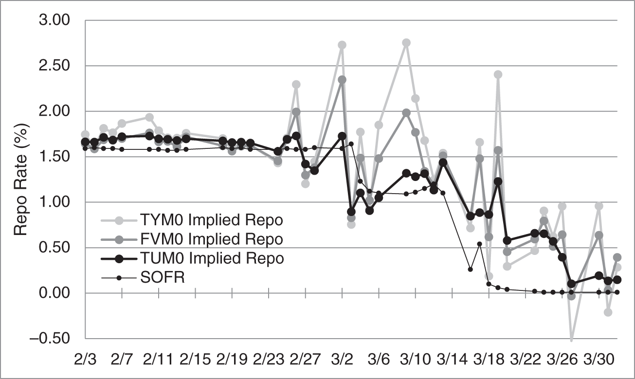
FIGURE 11.11 Implied Repo Rates of CTD Bonds into TYM0, FVM0, TUM0, and SOFR from February 3, 2020, to April 1, 2020.
Buying the basis at a negative price and holding the position until the net basis converges to zero had indeed, for some time, been a relatively reliable and stable money machine. From March 9, however, when Treasury yields became much more volatile, so did the P&L of long basis trades. The newfound volatility of the trade can be seen from the net and gross basis of TYM0 in Figure 11.10 and from the implied repo of TYM0, FVM0, and TUM0 in Figure 11.11. The market dislocations at that time can also be seen from rising spreads between CTD yields and the yields of nondeliverable, but otherwise comparable bonds. The TUM0 line in Figure 11.12 shows the difference between the yields of the 1.875s of 02/28/2022 and the CTD into TUM0, that is, the 2.375s of 03/15/2022. While these two bonds traded at a low and stable spread through February and early March, that spread rose and became much more volatile over the rest of March. Similarly behaved are the FVM0 and TYM0 spreads, that is, the spread between the 1.875s of 08/31/2024 and the CTD into FVM0, that is, the 1.25s of 08/31/2024, and the spread between the 2s of 11/15/2026 and the CTD into TYM0, that is, the 2.25s of 02/15/2027. Generally speaking, liquidity is in high demand when markets are volatile, and the most liquid bonds tend to trade at a premium. CTD bonds, which inherit the liquidity of their associated futures contracts, trade in volatile markets at a premium relative to bonds that – in normal times – are comparable. This premium, however, like the demand for liquidity, can be quite volatile, as evident from Figure 11.12.

FIGURE 11.12 Richness of CTD Bonds into TYM0, FVM0, and TUM0 Relative to Comparable, Non‐Deliverable Bonds, from February 3, 2020, to April 1, 2020.
TABLE 11.9 A $1 Billion Long TYM0 CTD Basis Trade, from March 6, 2020, to March 12, 2020. Net Basis Is in Ticks (32nds). All Other Columns Are in Dollars.
| Net | Daily | Cumulative | Margin per | Margin | Cumulative | |
|---|---|---|---|---|---|---|
| Date | Basis | P&L | P&L | Contract | Call | Cash |
| 03/06/2020 | −8.33 | 1,275 | –10,171,597 | |||
| 03/09/2020 | –18.48 | –3,172,148 | –3,172,148 | 1,375 | –797,772 | –14,141,517 |
| 03/10/2020 | –11.22 | 2,268,613 | –903,535 | 1,375 | 0 | –11,872,904 |
| 03/11/2020 | –5.70 | 1,725,636 | 822,101 | 1,600 | –1,794,988 | –11,942,256 |
| 03/12/2020 | –0.47 | 1,633,228 | 2,455,330 | 1,600 | 0 | –10,309,028 |
Long basis trades seem riskless, so long as they can be held to expiration. Through volatile markets, however, traders might not actually be able to maintain their positions. To illustrate, Table 11.9 describes a $1 billion long TYM0 CTD basis trade initiated at ![]() 8.33 ticks on March 6, 2020, and held through March 12, 2020. The table assumes that a trader buys $1 billion face amount of the bonds; sells a conversion‐factor weighted and tailed number of futures contracts, in this case, 7,978 contracts;13 and sells the CTD repo to the expiration of the contract. For this trade, therefore, as explained earlier in the chapter, the daily P&L, measured as of the delivery date, equals the change in the net basis times the $1 billion face amount of the bond position.
8.33 ticks on March 6, 2020, and held through March 12, 2020. The table assumes that a trader buys $1 billion face amount of the bonds; sells a conversion‐factor weighted and tailed number of futures contracts, in this case, 7,978 contracts;13 and sells the CTD repo to the expiration of the contract. For this trade, therefore, as explained earlier in the chapter, the daily P&L, measured as of the delivery date, equals the change in the net basis times the $1 billion face amount of the bond position.
The net basis closed at about ![]() 18.5 ticks on March 9, generating a loss of about $3.2 million. This is a sizable loss given that the target horizon profit of the trade is only the original 8.33 ticks, that is, (8/32)% times $1 billion, or $2.5 million. Many hedge funds manage risk, at least in part, by loss limits, and a loss of this magnitude might result in a trader being forced to exit the position. From then on, Table 11.9 reports that the trade makes money, as the net basis rises to nearly zero. By reporting only daily closes, however, the table minimizes the true volatility of the trade: a trader might be forced out of the positions because of a large, adverse intraday change in the net basis.
18.5 ticks on March 9, generating a loss of about $3.2 million. This is a sizable loss given that the target horizon profit of the trade is only the original 8.33 ticks, that is, (8/32)% times $1 billion, or $2.5 million. Many hedge funds manage risk, at least in part, by loss limits, and a loss of this magnitude might result in a trader being forced to exit the position. From then on, Table 11.9 reports that the trade makes money, as the net basis rises to nearly zero. By reporting only daily closes, however, the table minimizes the true volatility of the trade: a trader might be forced out of the positions because of a large, adverse intraday change in the net basis.
Another way a trader might be forced out of the basis trade is the need to come up with cash. As of March 6, with maintenance margin at $1,275 per contract, the short of 7,978 contracts requires posting a bit more than $10 million to the exchange.14 With the trade losing money on March 9, the hedge fund needs to make daily settlement payments on the futures contracts and variation margin payments on the term repo positions, which essentially sum to the P&L for the day, that is, to about $3.2 million. In addition, because of increased market volatility, the exchange increased the margin requirement from $1,275 to $1,375 per contract, generating a margin call of nearly $800,000. In total, then the hedge fund has to come up with an additional $4 million on March 9. This is a very large number relative, once again, to the target profit of $2.5 million. These cash requirements also clarify the concreteness of allocated capital, because that capital really does need to be available to meet the cash requirements of the trade. In any case, as the trade makes money after March 9, cash requirements fall, but not as quickly as indicated by the P&L; the exchange increased margin requirements once again on March 11.
A final way a trader might be forced out of a basis trade applies only to those that finance the bond purchases with overnight rather than term repo. In calm markets, rolling over overnight repo is nearly equivalent to term repo. More precisely, if the term repo rate reflects future, unchanging overnight rates, and if financing is plentiful, then there is no important difference in borrowing overnight and borrowing term. In more volatile markets, however, borrowing overnight adds two significant sources of risk.
First, the overnight rate can rise or fall relative to what could have been locked in to term. In March 2020, as shown in Figure 11.13, the overnight repo rate, as represented by SOFR, declined precipitously as the Federal Reserve lowered rates to accommodate market conditions. Bearing this risk actually worked in favor of traders who had not locked in term repo rates – with one caveat to be discussed presently – as they could roll overnight repo at lower and lower rates. Another way to express the advantage of not locking in term rates is to compare the gross and net basis of TYM0 in Figure 11.10. As the repo rate falls, the carry of the CTD increases, which means that its gross basis increases relative to its net basis.
Second, in stressed markets, prime brokers might reduce risk by limiting lending to hedge funds in the basis trade, or, with similar effect, by increasing repo haircuts. In that case, basis traders who did not lock in term repo might have to reduce position size or even exit a position at a loss. Some evidence of this funding risk through March 2020 can be seen from the difference between the 99th percentile repo rate and SOFR in Figure 11.13. Through February, the spread of the highest rate percentile of repo transactions over the median SOFR rate was typically only 10 or 11 basis points. In March, however, that spread was between 20 and 50 basis points on several days and hit a peak of 174 basis points on March 16. These data strongly imply that at least some overnight repo borrowers had trouble borrowing money against Treasuries. Furthermore, basis traders who had not locked in term rates might very well have had to roll over borrowing at rates very much above term rates they might have locked in at an earlier date.

FIGURE 11.13 SOFR and 1st and 99th Percentile Repo Rates, from February 3, 2020, to April 1, 2020.
NOTES
- 1 This graph is Figure 1 of Baker, L., McPhail, L., and Tuckman, B. (2018), “The Liquidity Hierarchy in the US Treasury Market,” Commodity Futures Trading Commission, December 3.
- 2 This terminology can be confusing because it differs from that of spot settlement. Most notably, the “value of a bond” is typically used interchangeably with the “bond price.”
- 3 An historical reason for daily settlement is the mitigation of counterparty risk. Because forwards can accumulate value over time, there can be significant exposure to a counterparty default. With futures, by contrast, exposure is limited to one daily settlement payment, because the contracts of a counterparty that defaults on a settlement payment are canceled. However, with modern practice usually requiring appropriate margin against forward contracts, the two types of contracts no longer differ qualitatively with respect to counterparty risk.
- 4 The covariance of two random variables is the product of their correlation and their two standard deviations. For the covariance to be high, therefore, the variables must be both highly correlated and highly volatile.
- 5 The terminology has become even more confusing with interest rate swaps being either collateralized‐to‐market or settled‐to‐market. See Chapter 13.
- 6 This bond was chosen as the example because it matures in an exact number of semiannual periods. For the other deliverable bonds, use the price‐yield Equation (A3.5).
- 7 As noted already, “carry” in the futures context is “cash carry” as defined in Chapter 3.
- 8 The definition of implied repo ignores the futures‐forward price difference.
- 9 On May 14, 2021, the yield of the 2.875s of 05/15/2028 was 1.26%; the yield of the 1.125s of 02/15/2031 was 36.5 basis points higher, at 1.625%; and the repo rate was 124.5 basis points below, at 0.015%. These are the spreads kept fixed in the figure.
- 10 To avoid confusion in terminology, note that many practitioners refer to the difference between the matching notional amount and the conversion‐factor weighted number of contracts as a “tail,” but this hedging adjustment is not at all related to “tailing the hedge” to account for the timing of daily settlement payments.
- 11 Note that the net basis in Figure 11.10 and the implied repo rate in Figure 11.11 assume that the term repo rate on each day equals the overnight repo that day. This is not a great assumption but is necessitated in this case by the lack of data on term repo rates.
- 12 Assigned capital in this context is an allocation from a fund's scarce risk and funding resources to one of its various trading or investment strategies. As the following discussion shows, capital assigned in this way must be available in ready funds should the need arise.
- 13 At $100,000 face amount per contract, 10,000 contracts is equivalent to the $1 billion face amount of bonds. The conversion factor of the CTD into TYM0 is 0.8006, the repo rate is 1.10%, and there are 116 days from March 6, 2020, to June 30, 2020. Therefore, the conversion‐factor weighted and tailed number of contracts is
 .
. - 14 Treasury repo does typically require margin, given in Table 10.3 at about 2%. However, because the risks of futures and bond positions in a basis trade are largely offsetting, a prime broker might very well – at least in normal times – not require a hedge fund to post much more than exchange‐required futures margin. The text assumes this even though, for some clients, prime brokers will require a cushion above exchange margin.