
CHAPTER 12
Short‐Term Rates and Their Derivatives
Short‐term funds trade in money markets in significant volumes and at a variety of interest rates. Interest rates vary across currencies, of course, but even within a single currency there are typically several rates that reflect differences in collateral, market participants, and term. This chapter introduces some of the most important short‐term interest rates across currencies and describes the global transition away from LIBOR. The chapter then describes a number of interest rate derivatives contracts – one‐month SOFR futures, fed funds futures, three‐month SOFR futures, Euribor FRAs, and Euribor futures – and explains their use in hedging exposures to short‐term interest rates. A detour shows how combining fed funds futures prices with Federal Reserve Board meeting dates is used to imply expectations of the Federal Reserve's target rate and to construct benchmark interest rate curves for general use. The chapter concludes with a brief discussion on the difference between futures and forward rates. Notes on pricing rate forwards and futures on rates with term structure models can be found in the appendix to Chapter 12.
12.1 SHORT‐TERM RATES AND THE TRANSITION FROM LIBOR
Since a first trade in 1969,1 LIBOR (London Interbank Offered Rate) grew to become the dominant set of reference rates for short‐term interbank borrowing. Across a wide variety of loans and derivatives, huge volumes of cash flows were set based on LIBOR. LIBOR rates were published daily for five currencies (CHF, EUR, GBP, JPY, USD) and for seven maturities (overnight, one week, one month, two months, three months, six months, 12 months), although the three‐month and to a much lesser extent the one‐month terms were the most popular. For each currency, a panel of 16 banks was surveyed with the question, “At what rate could you borrow funds, were you to do so by asking for and then accepting interbank offers in a reasonable size just prior to 11 a.m. (London time)?” The LIBOR fixing for each currency and term was then set equal to a trimmed mean of the survey responses.
In the wake of the quantitative easing policies of central banks after the financial crisis of 2007–2009, the survey methodology began to lose credibility. First, because banks with abundant reserves do not need to borrow reserves from other banks, the volume of interbank transactions fell so dramatically that survey responses became more subjective. Second, from 2012 to 2016, investigations revealed that traders at the panel banks colluded to manipulate LIBOR fixes to their advantage. Some traders were sentenced to prison, and banks collectively paid more than $9 billion in fines.
In 2017, regulators decided to terminate LIBOR and its use by the end of 2021. Furthermore, after consultations with industry representatives, it was decided that financial contracts in the future should reference a set of overnight, “risk‐free rate” (RFR) benchmarks, which can be set objectively based on large volumes of transactions data. The phrase “risk‐free rates” is somewhat of a misnomer, as only two of the new benchmarks – SARON in CHF and SOFR in USD – are based on collateralized repo rates, while the other three – €STR in EUR, SONIA in GBP, and TONAR in JPY – remain interbank rates. And although all of the new benchmarks are overnight rates, regulators have permitted the continued use of two term rate indexes, after methodological reforms, namely, Euribor in EUR and TIBOR in JPY. Table 12.1 and the following discussions outline the rates used before the transition and the RFRs compliant with post‐transition regulatory principles. The table highlights in bold the overnight benchmarks in each currency that are preferred by the regulators.
TABLE 12.1 Global Market Short‐Term Interest Rates, Pre‐ and Post‐ the Transition Away from LIBOR.
| Post‐Transition | ||||
|---|---|---|---|---|
| Interbank (Unsecured) | ||||
| Currency | Pre‐Transition | Repo | Overnight | Term |
| CHF | LIBOR | SARON (2009) | ||
| EUR | EONIA, Euribor | €STR (2019) | Euribor | |
| GBP | LIBOR, SONIA | SONIA | ||
| JPY | LIBOR, TIBOR, | TONAR (2016) | TIBOR | |
| Euroyen TIBOR | ||||
| USD | fed funds, LIBOR | SOFR (2017) | fed funds | Ameribor |
| BSBY | ||||
CHF: Swiss franc; EUR: euro; GBP: British pound; JPY: Japanese yen; USD: US dollar.
- Swiss Franc (CHF). The CHF benchmark moved from LIBOR to SARON (the Swiss Average Rate ON, where ON stands for overnight). SARON is a volume‐weighted average of the rates on general collateral, fixed income repo transactions. SARON is calculated a few times per day, along with indexes for several other terms (e.g., SAR1W for one week, and SAR3M for three months), but SARON at each day's close is the main benchmark rate.
- Euro (EUR). EONIA (Euro ON Index Average) was a volume‐weighted average of rates on overnight interbank loans, which was computed from transactions supplied by a panel of banks. Over time, the total volume of transactions, along with the number of banks in the panel with significant volumes, had fallen too much for the index to remain tenable. Euribor (Euro Interbank Offered Rate) had been a set of five term rates (one week, one month, three months, six months, 12 months) based on submitted quotations by panel banks, like LIBOR, although with a different administrator. As part of the transition away from LIBOR, Euribor was reformed in 2019 to follow a “hybrid methodology,” which, to the extent available, uses Level 1 contributions, which consist of wholesale funding transactions of panel banks – 18 at the time of this writing – on a given day and for a given term. To the extent such transactions are not available, Euribor may rely on Level 2 contributions, which are recent transactions at other terms, or, if necessary, on Level 3 contributions, which are relevant transactions from other, closely related markets. Perhaps not surprisingly, given the monetary regime of abundant reserves, a significant fraction of contributions are, indeed, Level 3.2 ESTR, ESTER, or €STR (Euro Short‐Term Rate) is the index favored by regulators. It is a volume‐weighted trimmed mean of sizable, overnight funding transactions by – at the time of this writing – 32 euro‐area banks.
- British Pound (GBP). SONIA (Sterling ON Index Average) has existed since 1997, has a history of use as a reference rate for derivatives transactions, and was reformed in 2018. Like €STR, the reformed SONIA is a volume‐weighted trimmed mean of sizable overnight bank funding transactions.
- Japanese Yen (JPY). There were two versions of TIBOR (Tokyo Interbank Offered Rate), both based on submissions by Japanese banks: Euroyen TIBOR, representing interbank JPY rates outside Japan (like JPY LIBOR), and JPY TIBOR or simply TIBOR, representing interbank JPY rates inside Japan. While Euroyen TIBOR has been abandoned, TIBOR was reformed in various ways in 2017, including – along the lines of the Euribor reforms – a waterfall of submission priorities, from actual interbank call or funding transactions, through data from similar or relevant markets, down to “Expert judgment,” though this last resort has not yet been necessary. TIBOR is published for five terms: one week, one month, three months, six months, and 12 months. TONAR (Tokyo ON Average Rate), also called TONA, was created in 2016 as a volume‐weighted average of transactions in the overnight call market.
- US Dollar (USD). fed funds is the overnight rate at which banks trade reserves at the Federal Reserve System. A further description of this market is given below. SOFR (Secured Overnight Financing Rate) is a trimmed, volume‐weighted median of overnight repo rates. Its calculation is described in more detail in Chapter 10. The other USD rates listed in Table 12.1 are discussed presently.
Given the enormous volume of loans and derivatives that had been referencing LIBOR, the transition to new rates, from an operational perspective, was time‐consuming and costly. Changes to derivatives markets were organizationally straightforward, in that regulators could push changes through a small number of clearinghouses and large dealers. By contrast, changes in loan markets required action by a large number of smaller banks. Particularly challenging in both markets, however, are legacy or existing contracts that reference LIBOR, but are difficult to change for various reasons, ranging from their being in structures that are hard to amend to their somewhat unresponsive counterparties. The resulting backlog of legacy contracts eventually forced regulators to postpone the cessation of a subset of LIBOR indexes. Five USD LIBOR tenors (overnight, one month, three months, six months, and 12 months) will continue to be published until June 30, 2022, for use by certain legacy contracts only. Three GBP and JPY LIBOR tenors (one month, three months, and six months) will continue to be published for legacy contracts for some time in synthetic form, which means that, instead of being calculated from survey results, as in the past, these LIBOR rates are now set as some fixed function of the preferred, post‐transition benchmarks, namely, SONIA and TONAR, respectively.
More substantive challenges to the transition, particularly in the loan market, arise from two key features of the new benchmarks. First, they are overnight rather than term rates. Second, they are rates with little to no bank credit risk. The challenge of moving from term to overnight rate benchmarks is described in Figure 12.1. Panel a) depicts the historical use of one‐month LIBOR as part of a longer‐term, floating‐rate loan. A borrower of $1 million from October 1 to November 1, 2021, knows the rate of interest at the start of the period and, therefore, can compute the interest due at the end of the period, in this case, ![]() . In this convention, interest is said to be set in advance of the loan period and paid in arrears of the loan period. With overnight rather than term benchmarks, however, borrowers typically do not know the final amount of interest at the start of the period. Panel b) shows the most straightforward structure for term loans with an overnight rate benchmark, namely, set in arrears and paid in arrears. Over the 31 days – October 1, 2021, to October 31, 2021 – SOFR was three basis points on three days, four basis points on one day, and five basis points on 27 days. On a $1 million loan, therefore, with daily compounding, the interest payment due at the end of the period is,
. In this convention, interest is said to be set in advance of the loan period and paid in arrears of the loan period. With overnight rather than term benchmarks, however, borrowers typically do not know the final amount of interest at the start of the period. Panel b) shows the most straightforward structure for term loans with an overnight rate benchmark, namely, set in arrears and paid in arrears. Over the 31 days – October 1, 2021, to October 31, 2021 – SOFR was three basis points on three days, four basis points on one day, and five basis points on 27 days. On a $1 million loan, therefore, with daily compounding, the interest payment due at the end of the period is,

FIGURE 12.1 Examples of Monthly Interest Payment Conventions for a $1 Million Monthly Resetting Floating‐Rate Loan, September to November 2021.

But the borrower does not know this amount until the end of the period, when all relevant SOFR rates have been observed. Many financial institutions, whose business is the money markets, might be perfectly comfortable with this uncertainty. Nonfinancial corporate borrowers, however, might not be comfortable with uncertain interest payments at the end of one‐month, three‐month, or longer reset periods.
There exist several operational fixes designed to give borrowers time to compute and make interest payments. A payment delay simply gives the borrower an extra day or so to make the payment. A lockout allows for earlier computation of interest payments by not using the very last rate settings. For example, a one‐day lockout might use the rate for October 30 for both October 30 and October 31. And a lookback uses earlier rather than the latest rates. In the present example, the observation period might be shifted from October 1 through October 31 to September 30 through October 30. These minor tweaks, however, do not change the fact that borrowers do not know how much they will pay in interest until sometime near the end of the period.
One proposed solution to this more significant challenge, depicted in Panel c) of Figure 12.1, is to use overnight rates in a set in advance, paid in arrears structure. For example, to determine the payment on November 1, 2021, use the interest rates from September 1 to October 1 (inclusive). Over this period, SOFR was five basis points every day, giving an interest payment of ![]() . In this way, the borrower does know the interest due on November 1 as of October 1. The reference interest rates, however, do not correspond to the borrowing period, which may or may not be important depending on the situation and on the structure of any complementary positions.
. In this way, the borrower does know the interest due on November 1 as of October 1. The reference interest rates, however, do not correspond to the borrowing period, which may or may not be important depending on the situation and on the structure of any complementary positions.
The most natural solution, from a theoretical perspective, is for the market to develop term rates, based on the benchmark overnight rates, for use in loans to borrowers who want payment certainty. Some such term rates are, in fact, in use for some purposes, including the synthetic versions of GBP and JPY LIBOR mentioned already. And the CME, a major US derivatives clearinghouse, has been encouraged to create term SOFR rates for limited use. For now, however, regulators are discouraging – as a return to the recent weaknesses of LIBOR – the broad use of term rates that are not directly observable from significant volumes of market transactions. In the future, perhaps, the rate derivatives described later in the chapter will trade with enough liquidity to provide acceptable term rates.
The second substantive challenge to the LIBOR transition is that the new RFR benchmarks embed little to no bank credit risk. In the heyday of LIBOR, banks would borrow funds at LIBOR or at a spread to LIBOR and would lend funds to customers at LIBOR plus a spread. Banks were naturally hedged, therefore, against increases in the cost of funds of the banking sector. Some of the new overnight benchmarks are interbank rates, namely, €STR, SONIA, and TONAR, but overnight interbank rates – as opposed to term interbank rates – do not typically fluctuate much with credit conditions until well into a financial crisis. And the other two new benchmarks, SARON and SOFR, are based on repo rates, which, if anything, might fall as credit conditions worsen, as flight‐to‐quality trades flock to safer lending havens. The question for the transition, therefore, is whether banks will benchmark large volumes of their customer loans to RFRs, and even if they do so in normal times, will they continue to do so in times of stress.
In EUR and JPY, the continued use of term Euribor and TIBOR enables the use of credit‐sensitive rates (CSRs). In the United States, there are two suites of rates that have been deemed by independent auditors as compliant with international regulatory principles pertaining to benchmarks. Ameribor (American Interbank Offered Rate) is computed for a range of terms from the funding transactions and executable quotes of a large number of small to regional US banks on the American Financial Exchange (AFX). BSBY (Bloomberg Short‐Term Bank Yield Index) is computed for a range of terms from the funding transactions and executable quotes of large banks across the Bloomberg trading platform. Futures contracts are listed on both Ameribor and BSBY rates. AXI (Across‐the‐Curve Credit Spread Index) is not listed in Table 12.1, because, at the time of this writing, it had not yet been deemed compliant with regulatory benchmark principles. This index is intended as a credit spread to be added to SOFR, is available for a range of terms, and is based on unsecured bank funding transactions. Ameribor, BSBY, and AXI, from a commercial perspective, face not only the normal challenges in bringing new products to market but also the regulatory headwinds that support broad adoption of SOFR.3
12.2 ONE‐MONTH SOFR FUTURES
The one‐month SOFR futures contract, which trades on the CME (Chicago Mercantile Exchange), is designed to take and hedge exposure to SOFR or to other rates believed to be highly correlated with SOFR. Selected one‐month SOFR contracts, along with their prices and rates as of January 14, 2022, are given in Table 12.2. Each ticker is composed of the code “SER,” a letter indicating the contract month, and a digit corresponding to the last digit of the contract year. For example, with “G” standing for February, SERG2 is the ticker for the one‐month SOFR contract of February 2022. Its current price is 99.935, which corresponds to a percentage rate of ![]() , or 0.065. Expressing the percentage rate as 100 minus price is just a convention: there is no sense in which the price of a particular bond or other instrument at a rate of 0.065% equals 99.935.4
, or 0.065. Expressing the percentage rate as 100 minus price is just a convention: there is no sense in which the price of a particular bond or other instrument at a rate of 0.065% equals 99.935.4
TABLE 12.2 Selected One‐Month SOFR Futures Contracts, as of January 14, 2022. Rates Are in Percent.
| Ticker | Month | Price | Rate |
|---|---|---|---|
| SERF2 | Jan | 99.9475 | 0.0525 |
| SERG2 | Feb | 99.935 | 0.065 |
| SERH2 | Mar | 99.815 | 0.185 |
| SERJ2 | Apr | 99.685 | 0.315 |
| SERK2 | May | 99.585 | 0.415 |
Each contract trades until the last business day of the month in which it expires, known as its delivery month. The word “delivery” here is a carryover from other futures contracts, which, at expiration, require the delivery of an underlying commodity or financial instrument in exchange for some payment. SOFR contracts, however, are cash settled; that is, they require no physical delivery at expiration.
The final settlement rate of a one‐month SOFR contract equals the average SOFR rate over that month. Each day of the month is included in the average, and non‐business days take the rate of the previous business day. For example, the SOFR rate for Friday, February 4, 2022, is counted three times in the February average: once for Friday, February 4; once for Saturday, February 5th; and once for Sunday, February 6th. The final settlement price of a contract equals 100 minus the percentage rate. If, for example, the average SOFR rate over the month of February 2022 is 0.09%, then the final settlement price is ![]() , or 99.91.5
, or 99.91.5
The one‐month SOFR contract is scaled to hedge a $5 million 30‐day investment. More specifically, the P&L (profit and loss) on one contract from a one‐basis‐point decrease in the contract's rate is set equal to,
To elaborate on the P&L from buying, holding, and selling this futures contract, consider a trader that buys one February contract on January 14, 2022, at a price of 99.935, which corresponds to a rate of 0.065%. Say further that the price falls to 99.910, or equivalently, that the rate rises to 0.09%, and that the trader either sells the contract or that the contract expires at those levels. Because the trader bought the contract and the price fell, the trader loses money. The actual loss is determined with reference to Equation (12.2). Because the contract rate rose from 0.065% to 0.09%, that is, by 2.5 basis points, the trader loses 2.5 times $41.67, or $104.175. If, the price rises instead, the buyer of a contract makes money. More specifically, if the price rises from 99.935 to 99.995, or, equivalently, the rate falls by six basis points, then the P&L from the purchase of one contract is six times $41.67, or $250.02.
Like other futures contracts, one‐month SOFR contracts are subject to daily settlement payments. Futures prices fluctuate throughout the day, according to market forces, and, at the end of each day, the exchange sets a settlement price, which usually equals the price of the last trade. All market participants then settle up their gains and losses over the day. Those who were long one‐month SOFR contracts over the day pay $41.67 for every one‐basis‐point increase in rates over the day or receive $41.67 for every one‐basis‐point decrease in rates over the day. Correspondingly, those who are were short over the day receive $41.67 for every one‐basis‐point increase in rates or pay $41.67 for every one‐basis‐point decrease in rates.6
Because of daily settlement payments, the P&L of a futures position is realized over its holding period rather than all at unwind or at final settlement. In one of the previous examples the February contract is bought on January 14 at a rate of 0.065% and expires or is sold at a rate of 0.005%, for a six‐basis‐point or $250.02 gain. That gain is realized over time: daily settlement payments are made on days when rates rise and are received on days when rates fall. The sum of all those daily settlement payments, however, corresponds to the overall six‐basis‐point decline in rates, that is, to an overall profit of $250.02. The exact pattern of gains and losses over the holding period does not matter much when interest rates are very low, as they have been for several years. In higher rate environments, however, the pattern does matter. For winning positions, early gains, which can be reinvested, can be worth significantly more than later gains. Similarly, for losing positions, early losses, which have to be financed, can cost significantly more than later losses. The implications of daily settlement are discussed further presently.
The stage is now set for a simple example of hedging with one‐month SOFR contracts. Consider a money market fund that plans to invest $50 million from January 14 to March 14, 2022, in overnight repo. The fund chooses overnight repo because of its liquidity, that is, its ready availability in the contingency of larger than anticipated requests to redeem shares. At the same time, however, the fund decides to hedge the interest rate risk of falling repo rates with one‐month SOFR futures. More specifically, to offset losses from falling repo rates, the fund buys one‐month SOFR futures contracts, which profit from falling repo rates. The question for the fund then, is which contracts and how many to buy.
Focusing first on hedging the risk of falling repo rates over the month of February, the fund can buy February contracts. Because each contract is scaled to hedge a $5 million 30‐day investment, while the fund is investing $50 million over the 28‐day month of February, the fund needs to buy,

contracts. Under a few simplifying assumptions, discussed presently, the performance of this hedge is described in Table 12.3. The first column gives the average realized rate over the month of February. The second column gives the investment proceeds from earning simple interest in repo over the month of February. At an average repo rate of 0.09%, for example, the fund earns $50 million × ![]() . The third column gives the P&L from being long 9.33 contracts. Taking again the realized average rate of 0.09%, which is 2.5 basis points above the purchase rate of 0.065%, the long futures position loses
. The third column gives the P&L from being long 9.33 contracts. Taking again the realized average rate of 0.09%, which is 2.5 basis points above the purchase rate of 0.065%, the long futures position loses ![]() . The fourth column gives the net proceeds, that is, the sum of the investment proceeds and the P&L from the SOFR futures hedge. The hedge works well in the sense that, no matter what the realized average rate, net proceeds are about the same. To elaborate, buying SOFR futures at a rate of 0.065% approximately locks in a net P&L of $2,528. If the realized repo rate is less than 0.065%, investment proceeds are less, but futures P&L profits compensate for the difference. If the realized repo rate is greater than 0.065%, investment proceeds are greater, but futures P&L losses offset the difference. The reader can verify that the hedge works perfectly, that is, net proceeds always equal $2,527.78, under the contrafactual assumptions that: i) the fund buys exactly 9 1/3 contracts, which is the exact solution of Equation (12.3); and ii) the P&L of the futures contract is exactly $41 2/3 per basis point, which is the exact expression in Equation (12.2).
. The fourth column gives the net proceeds, that is, the sum of the investment proceeds and the P&L from the SOFR futures hedge. The hedge works well in the sense that, no matter what the realized average rate, net proceeds are about the same. To elaborate, buying SOFR futures at a rate of 0.065% approximately locks in a net P&L of $2,528. If the realized repo rate is less than 0.065%, investment proceeds are less, but futures P&L profits compensate for the difference. If the realized repo rate is greater than 0.065%, investment proceeds are greater, but futures P&L losses offset the difference. The reader can verify that the hedge works perfectly, that is, net proceeds always equal $2,527.78, under the contrafactual assumptions that: i) the fund buys exactly 9 1/3 contracts, which is the exact solution of Equation (12.3); and ii) the P&L of the futures contract is exactly $41 2/3 per basis point, which is the exact expression in Equation (12.2).
TABLE 12.3 Hedging a $50 Million Overnight Repo Investment with 9.33 One‐Month February SOFR Futures Contracts, Purchased at a Rate of 0.065%, as of January 14, 2022. Rates and in Percent. Other Entries Are in Dollars.
| Realized | Investment | Futures | Net |
|---|---|---|---|
| Avg. Rate | Proceeds | P&L | Proceeds |
| 0.050 | 1,944.44 | 583.17 | 2,527.62 |
| 0.065 | 2,527.78 | 0.00 | 2,527.78 |
| 0.090 | 3,500.00 | −971.95 | 2,528.05 |
The depiction of the hedge in Table 12.3 is simplified in several ways. First, the fund has to buy a whole number of contracts, that is, nine (or 10) rather than 9.33. This is less of an issue, of course, for larger hedges, and another practical solution to this rounding problem is discussed presently. Second, the table ignores interest on daily settlement payments, which is negligible when rates are very low and the time horizon is short. Third, it is assumed that investment proceeds earn simple interest, whereas interest is more likely to compound. This effect, too, is small when rates are low and the horizon short. Fourth, the table assumes that the average repo rate that determines the fund's investment proceeds is exactly the same as the average SOFR rate that determines the final settlement rate of the futures contract. While extremely reasonable, this assumption may not hold exactly in practice. SOFR on any day is the trimmed median rate of all transactions that day. The fund, on the other hand, executes its own repo transactions each day at a particular time with a particular dealer.
Stepping back to the full example, the money market fund wants to hedge its overnight repo investments from January 14 to March 14. The hedge over February is described above. Turning to the hedge over the month of January, note that SOFR observations for the first 13 days of January have already been set. Therefore, a one‐basis‐point change to repo rates over each of the remaining 18 days of January moves average SOFR for the month by only 18/31 basis points. Similarly, the fund is investing in repo over only 18 days in January. The correct number of contracts for the hedge is, therefore,
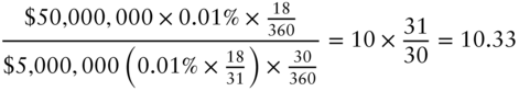
In words, because the number of remaining days in the month affects the investment proceeds and the futures contract in the same way, the fact that the hedge starts in the middle of the month can be ignored. Therefore, just as in Equation (12.3) for the February hedge, the number of contracts for the January hedge is the investment of $50 million for 31 days divided by the contract's effective hedge of $5 million for 30 days, which equals 10 times 31/30, or 10.33. Table 12.4 illustrates the January hedge, noting that SOFR over each of the first 13 days of January was five basis points. The format of the table is similar to that of Table 12.3, but the first column is the average repo rate over the whole month, which determines the futures P&L, while the second column is the average repo rate over the last 18 days of the month, which determines the investment proceeds. From the first row, for example, the first 13 days at five basis points and the last 18 days at 2.85 basis points give an average over the month of ![]() basis points.
basis points.
TABLE 12.4 Hedging a $50 Million Overnight Repo Investment with 10.33 One‐Month January SOFR Futures Contracts, Purchased at a Rate of 0.0525%, as of January 14, 2022. SOFR Was 0.05% on Every Day from January 1 to 13. Rates Are in Percent. Other Entries Are in Dollars.
| Jan 1‐31 | Jan 14‐31 | |||
|---|---|---|---|---|
| Realized | Realized | Investment | Futures | Net |
| Avg. Repo | Avg. Repo | Proceeds | P&L | Proceeds |
| 0.0375 | 0.0285 | 711.81 | 645.68 | 1,357.48 |
| 0.0525 | 0.0543 | 1,357.64 | 0.00 | 1,357.64 |
| 0.0775 | 0.0974 | 2,434.03 | −1,076.13 | 1,357.90 |
Table 12.4 shows that the January hedge performs as expected. The January SOFR futures price is at a rate of 0.0525%, which implies a rate of 0.0543% over the last 18 days of the month. The money market fund can lock in the investment proceeds at this rate, that is, $50 million × 0.0543% × 18/360, or about $1,358. At lower realized rates, investment proceeds are lower, but futures gains compensate. At higher realized rates, investment proceeds are higher, but are given back through futures losses. Note that, as in the previous table, the hedge would work exactly for 10 1/3 contracts and a futures profit or loss of $41 2/3 per basis point.
The discussion of this January hedge reveals, more generally, that hedges with one‐month SOFR futures from any date within a month to the end of that month require no special handling. Hedge ratios are computed as if the entire month were being hedged, and, consequently, hedge ratios do not change over the course of the contract month. Applying this conclusion to the February part of the hedge, described earlier, the fund maintains its initial long of 9.33 contracts throughout the entire month of February, after which time those contracts expire.
The remaining piece of the overall money market fund hedge is using the March contract to hedge repo rates from March 1 to 13, which rates determine the fund's investment proceeds from March 1 to the assumed horizon date of March 14. Proceeding in the same way as for January and February, the fund would hedge its $50 million investment over 13 days with contracts that hedge $5 million over 30 days by buying 10 times 13/30, or 4.33 March contracts. With the rate of the March contract at 0.185% as of January 14, this approach would seemingly lock in a repo investment rate of 0.185%. It is left to the reader to construct a table like Tables 12.3 and 12.4 to illustrate this point. The March hedge is actually more complicated than the January and February hedges, however, for two reasons. First, 4.33 contracts are appropriate from January 14 until before the setting of SOFR on March 1, but not for the rest of March. Consider, for example, the hedge on March 4, before the setting of SOFR on that day. There are 10 days left of exposure to the investment – March 4 to March 13, inclusive of both dates – and 28 days left of exposure to the contract – March 4 to March 31, inclusive of both dates. The hedge ratio, therefore, is given by,

In short, the appropriate number of contracts falls gradually over March from 4.33 before the setting of repo on March 1 to zero on March 14. More generally, the number of one‐month SOFR contracts hedging exposure from the beginning of the month to sometime within the month declines over the course of the month.
The second and more serious problem with the proposed March hedge is its implicit assumption that repo rates in the first 13 days of March move in parallel with rates over the whole month. In fact, the Federal Reserve announces on March 16, 2022, whether it is or is not raising its short‐term policy rates. The problem for the money market fund in the example, then, is the scenario in which the market raises its expectation for a policy rate increase on March 16. In that case, rate expectations for the second half of March rise; the SOFR March contract rate rises and its price falls; the money market fund loses money on its futures hedge; but, because repo rates do not rise before the policy change, in the first half of March, fund investment proceeds do not rise.
In this particular example, there is a reasonable solution to the problem of the March hedge: hedge the exposure to repo interest rates from March 1 to March 13 with February SOFR contracts! The prior scheduled announcement of Federal Reserve policy rates is on January 26. Much of the fund's exposure to repo rates in the first part of March, therefore, is captured by February SOFR contracts, which incorporate expectations and realized policy decisions from the January meeting. Therefore, instead of purchasing 4.33 March contracts at the start of the hedge, on January 14, the fund can purchase an additional 4.33 February contracts. Of course, at the end of February, when the contracts expire, the fund is faced with another decision. It can essentially roll the hedge from February to March contracts, by purchasing 4.33 March contracts as the 4.33 February contracts expire. Or the fund might decide that the basis risk between changes in rates over the first part of March relative to changes in rates over the whole of March is large relative to the risk of repo rates moving much before the scheduled March policy meeting. In that case, the fund might choose not to hedge. In any case, the strategy of stacking the fund's March risk into February contracts is not a cure‐all: some economic and financial surprises might affect repo rates in February, but not in the first part of March, while other surprises might affect repo rates in the first part of March, but not in February. All in all, however, the risk of rates changing over the policy meeting is likely the most important consideration, which argues for stacking into February contracts.
TABLE 12.5 Two Hedging Strategies for a $50 Million Overnight Repo Investment with One‐Month SOFR Futures Contracts, as of January 14, 2022. There Is a Scheduled Federal Reserve Target Rate Policy Announcement on March 16, 2022.
| Month‐by‐Month | Stacking Mar into Feb | ||
|---|---|---|---|
| Ticker | Contract Month | Number of Contracts | Number of Contracts |
| SERF2 | Jan | 10.33 | |
| SERG2 | Feb | 13.67 | |
| SERH2 | Mar | 0.00 | |
| Total | 24.00 | 24.00 |
By way of summary, Table 12.5 describes the overall hedge strategies of the money market fund in this example. The $50 million amount being hedged and the number of days in each month, set against the $5 million 30‐day SOFR futures contract, give the number of contracts in the “Month‐by‐Month” strategy. Avoiding the basis risk of hedging the first part of March with all of March, and relying on the assumption that almost all repo rate variability arises from changes to policy target rates, the “Stacking Mar into Feb” strategy uses February contracts to hedge the risk from the first part of March.
The notion of stacking contracts with risks from other periods allows the discussion to circle back to the question of dealing with a fractional number of contracts. Table 12.5 shows that the total number of contracts required in either hedge is 24. To avoid fractional contracts, then, while keeping overall exposure correct, stack the fractional amounts from some months into others. In the Month‐by‐Month strategy, for example, the fund might divide the total 24 contracts into 10 January contracts, 10 February contracts, and 4 March contracts. In the “Stacking Mar into Feb” strategy, the fund might – to avoid too much idiosyncratic February risk – buy 11 January contracts and 13 February contracts. Any stacking strategy does expose the fund, however, to any idiosyncratic changes in rates that appear in one month, but not in another.
12.3 FED FUND FUTURES
Banks that have accounts at the Federal Reserve system can trade these fed funds with each other; that is, they can borrow from and lend to each other, at market‐determined rates, in the fed funds market. These trades are predominantly for overnight borrowing and lending, and the effective fed funds rate, calculated each day, is the volume‐weighted average of the overnight rates on fed funds traded that day.
Before the financial crisis of 2007–2009, under the monetary policy regime of scarce reserves, domestic commercial banks actively traded in the fed funds market to manage their individual shortages or surpluses of reserves. Furthermore, the Federal Reserve conducted monetary policy by adding or subtracting reserves from the system so as to keep effective fed funds at or very close to a policy target rate. More recently, however, in the regime of abundant reserves, domestic commercial banks do not need to borrow funds from each other; they face various regulatory incentives to hold reserve balances; and they earn interest on reserves held at the Federal Reserve. The resulting transformation of the fed funds market has been dramatic, both in terms of a significant decline in volumes and in terms of a change in the composition of market participants. Lending is now dominated by Federal Home Loan Banks (FHLBs) – that do not earn interest on their accounts at the Federal Reserve – and borrowing is now dominated by US subsidiaries of foreign banks – that typically do not take US deposits and are not constrained by the full range of US bank regulations. The fed funds market has thus become a means through which FHLBs can earn interest on their surplus cash in the Federal Reserve system, and foreign banks can earn a spread by borrowing from the FHLBs and depositing those borrowed funds into interest‐bearing accounts at the Federal Reserve.7
While the Federal Reserve no longer changes the quantity of reserves in the system to influence short‐term rates, it uses other policy tools to keep effective fed funds within a target range, defined by an upper and lower limit. Figure 12.2 graphs these upper and lower limits, along with the effective fed funds rate itself, from January 2010 to January 2022. Effective fed funds is somewhat volatile, but nearly always within the policy target range.
The fed funds effective rate is of interest to participants in the fed funds market; to those who borrow and lend at a spread over fed funds effective; to those who trade derivatives tied to fed funds effective; and to anyone taking positions on future Federal Reserve policy. For these groups, fed fund futures can be used to manage exposures to fed funds effective. These futures contracts can be explained concisely here, because one‐month SOFR futures, described in the previous section, are designed along the same lines. The final settlement rate of a fed fund futures contract in a particular delivery month is the average of fed funds effective over that month, with non‐business days taking on the previous business day's rate. Like one‐month SOFR futures contracts, price is quoted as 100 minus the percentage rate; contracts are subject to daily settlement; and contracts are scaled such that a one‐basis‐point change in the rate results in a daily settlement flow of $41.67. With all of these similarities to one‐month SOFR contracts, hedging with fed fund futures proceeds along the same lines as in the previous section. The text continues, therefore, with the use of fed fund futures to infer market expectations of Federal Reserve rate policy decisions.

FIGURE 12.2 Fed Funds Effective Rate and Target Range, January 2010 to January 2022.
Table 12.6 lists fed fund futures contracts, prices, and rates as of two dates: October 1, 2021, and January 17, 2022. The rightmost column of the table lists the meeting dates of the Federal Open Market Committee (FOMC), which, on the second day of each set of meetings, announces any monetary policy changes, including changes to the federal funds target rate. As explained in Chapter 8, forward interest rates are a combination of expected rates in the future and a risk premium, but the risk premium over a year is likely to be relatively small. Also, as explained later in this chapter, near‐term forward rates and futures rates are very similar. Therefore, roughly speaking, the one‐month fed fund futures rates in Table 12.6 can be viewed as market expectations of future monthly average effective fed funds. In this light, the main lesson from the table is that expectations of Federal Reserve policy changed significantly from October 1, 2021, to January 17, 2022. As of October 1, fed fund futures anticipated effective fed funds rising from eight basis points to 28 basis points by the end of 2022. As of January 17, 2022, however, by which time surging inflation had begun to worry Federal Reserve officials, fed fund futures anticipated effective fed funds rising from 8.25 basis points to 99.5 basis points by the end of 2022.
TABLE 12.6 Prices and Rates of Selected Fed Funds Futures Contracts, as of October 1, 2021, and January 17, 2022, and 2022 FOMC Meeting Dates. Rates Are in Percent.
| 10/1/2021 | 1/17/2022 | FOMC | ||||
|---|---|---|---|---|---|---|
| Ticker | Month | Price | Rate | Price | Rate | Meeting |
| FFV1 | Oct (2021) | 99.920 | 0.080 | |||
| FFX1 | Nov | 99.920 | 0.080 | 11/2‐3 | ||
| FFZ1 | Dec | 99.920 | 0.080 | 12/14‐15 | ||
| FFF2 | Jan (2022) | 99.925 | 0.075 | 99.9175 | 0.0825 | 1/25‐26 |
| FFG2 | Feb | 99.920 | 0.080 | 99.9050 | 0.0950 | |
| FFH2 | Mar | 99.920 | 0.080 | 99.7800 | 0.2200 | 3/15‐16 |
| FFJ2 | Apr | 99.920 | 0.080 | 99.6450 | 0.3550 | |
| FFK2 | May | 99.915 | 0.085 | 99.5500 | 0.4500 | 5/3‐4 |
| FFM2 | Jun | 99.900 | 0.100 | 99.4500 | 0.5500 | 6/14‐15 |
| FFN2 | Jul | 99.885 | 0.115 | 99.3450 | 0.6550 | 7/26‐27 |
| FFQ2 | Aug | 99.865 | 0.135 | 99.2800 | 0.7200 | |
| FFU2 | Sep | 99.845 | 0.155 | 99.2350 | 0.7650 | 9/20‐21 |
| FFV2 | Oct | 99.800 | 0.200 | 99.1450 | 0.8550 | |
| FFX2 | Not | 99.775 | 0.225 | 99.0650 | 0.9350 | 11/1‐2 |
| FFZ2 | Dec | 99.720 | 0.280 | 99.0050 | 0.9950 | 12/13‐14 |
Many market participants, in fact, use fed fund futures rates together with the FOMC meeting dates to build a market term structure of fed funds effective. The key assumption is that the Federal Reserve changes its target rate only at its scheduled meetings. This has been a good description of recent history, with only rare exceptions, like after the terrorist attacks on September 11, 2001, during the financial crisis in 2008, and in response to the COVID pandemic and economic shutdowns in March 2020. In any case, given this assumption, the idea is to find a set of forward rates, from one meeting to the next, that are more or less consistent with fed fund futures prices.
To illustrate the procedure, focus on January 17, 2022. Note that the fed funds effective rate was eight basis points from January 1 to January 17 (not shown in the table). The FOMC could announce a new target rate the afternoon of January 26 and, because there is no FOMC meeting in February, the rate set by the FOMC on January 26 will be the average fed funds effective rate in February. But the February contract rate is 0.095%. Hence, the market's expectation of fed funds effective after the January 26 meeting is 0.095%.8 To flesh out the meaning of this expectation, assume further, consistent with recent history, that the Federal Reserve will change the target rate by either zero or 25 basis points. Then, given a post‐meeting expected rate of 0.095%, the implied probability, ![]() , of a 25‐basis‐point increase in rate on January 26, from 8 to 8+25 or 33 basis points, is given by,
, of a 25‐basis‐point increase in rate on January 26, from 8 to 8+25 or 33 basis points, is given by,
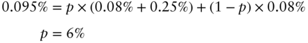
In words, with a 6% probability of the Federal Reserve increasing fed funds effective from eight to 33 basis points, and a 94% probability of leaving fed funds effective at eight basis points, the expected fed funds effective rate is 9.5 basis points, as implied by the February contract price.
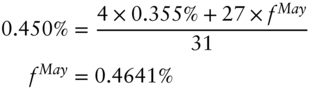
Moving to the next meeting, because there is a possible rate target announcement on March 16, but no meeting in April, the April futures rate of 0.355% indicates a market expectation of 0.355% after the announcement on March 16. Implying the results of the May meeting is more complex, because there is a meeting in June. Hence, to calculate the market's expectation of the May meeting, let ![]() be expected fed funds effective after the May meeting, which takes effect starting and including May 5. The May fed futures rate of 0.450%, therefore, is an average of four days at the expectation of 0.355% coming out of the previous meeting, and 27 days at
be expected fed funds effective after the May meeting, which takes effect starting and including May 5. The May fed futures rate of 0.450%, therefore, is an average of four days at the expectation of 0.355% coming out of the previous meeting, and 27 days at ![]() . Mathematically,
. Mathematically,
Continuing along these lines, the expected fed funds effective rate can be computed for each date. Figure 12.3 shows the results of this exercise, as of October 1 and as of January 17, using fed fund futures rates from Table 12.6. This figure graphically conveys the same message as the futures rates themselves, namely, that the market revised its rate expectation upward from October 1 to January 17. The figure, however, relying on the meeting dates, explicitly shows the path of expected rates.
This section concludes with an aside about curve building, that is, about mathematically representing the term structure of interest rates. Putting aside the small differences between short‐term futures and forward rates, discussed next, Figure 12.3 can be read as a flat‐forward‐rate representation of the term structure. In other words, the term structure of forward rates is represented as a sequence of constant forward rates. While this structure may seem odd from a purely economic perspective, because forward rates might be expected to change smoothly over time, flat forwards often represent all available market information. Fed fund futures, for example, provide only one rate per month. Furthermore, while flat forwards are discontinuous; that is, they jump at particular terms, they lead to relatively smooth spot rates and discount factors. To illustrate, using the relationships from Chapters 1 and 2, Figure 12.4 constructs weekly spot rates, discount factors, and forward rates from the flat forwards of Figure 12.3. These curves can reasonably be used to discount cash flows from other short‐term instruments of equivalent credit risk, or as a base curve above which spreads can be added to discount riskier cash flows.
In building curves, there is always a trade‐off between stability and smoothness. Flat forwards are very stable. Small changes in fed fund futures rates, for example, move flat forwards and corresponding spot rates or discount factors by small amounts and in sensible ways. Smooth representations of interest rate curves, however, like cubic splines, which are not described in this book, are notoriously unstable. Small changes in market rates in one part of the curve often lead to larger changes in other, relatively distant parts of the curve. Current industry practice favors more stable methodologies, like flat forwards, combined with an effort to collect as many market data points as possible, particularly in the short end of the curve. In general, the more market data, the less significant the discontinuities or jumps in the flat forward curve. Jumps between meeting dates, however, as in Figure 12.3, are actually a feature of the methodology, as they capture the financial reality of short‐term rates jumping after FOMC meetings.

FIGURE 12.3 Implied 2022 fed funds Effective Rates from Fed Fund Futures, as of October 1, 2021, and January 17, 2022.

FIGURE 12.4 A Term Structure of Weekly Interest Rates from Fed Fund Futures, as of January 17, 2022.
12.4 THREE‐MONTH SOFR FUTURES
Like one‐month SOFR futures, three‐month contracts are designed to hedge exposure to SOFR and are subject to daily settlement. There are three differences, however. First, and most obviously, three‐month contracts hedge exposure over three months, with the exact determination of dates described presently. Second, the settlement rate of the three‐month contract is based not on average SOFR over the reference period, but rather on daily compounded SOFR. Third, the three‐month contract is scaled to hedge a $1 million 90‐day investment, which means that the P&L on one contract from a one‐basis‐point decrease in the final settlement rate is set equal to,
Table 12.7 lists the first four three‐month contracts, along with their prices and rates, as of January 14, 2022. The first three letters of the ticker, “SFR,” denote the three‐month SOFR contract, while the following letter and digit, as for other futures contracts, denote the delivery month and last digit of the year. The “Start Date” of the reference period is the IMM (International Monetary Market) date corresponding to the contract month, where IMM dates are defined as the third Wednesday of March, June, September, and December. The “Last Trade Date” of a contract, which is also the last day of the reference period, is the business day before the next IMM date. And the “Valuation Date,” which is the day of the last daily settlement payment, is the business day after the last trade date. For the June three‐month SOFR contract, for example, the reference period for the calculation of the final settlement rate is from the June IMM date, or June 15, 2022, inclusive, to the September IMM date, or September 20, 2022, inclusive. The contract stops trading on September 20, 2022, and the last daily settlement payment is on September 21, 2022, which is the date that SOFR for September 20, 2022, is published.
TABLE 12.7 Selected Three‐Month SOFR Futures Contracts, as of January 14, 2022. Rates Are in Percent.
| Delivery | Start Date | Last Trade | Valuation | |||
|---|---|---|---|---|---|---|
| Ticker | Month | (inclusive) | Date | Date | Price | Rate |
| SFRZ1 | Dec | 12/15/2021 | 03/15/2022 | 03/16/2022 | 99.940 | 0.060 |
| SFRH2 | Mar | 03/16/2022 | 06/14/2022 | 06/15/2022 | 99.640 | 0.360 |
| SFRM2 | Jun | 06/15/2022 | 09/20/2022 | 09/21/2022 | 99.350 | 0.650 |
| SFRU2 | Sep | 09/21/2022 | 12/20/2022 | 12/21/2022 | 99.125 | 0.875 |
Let ![]() denote SOFR for date
denote SOFR for date ![]() , and let
, and let ![]() denote the total number of days in the reference period. As in the cases of one‐month SOFR futures and fed fund futures, SOFR for any non‐business day is taken as the value of SOFR on the previous business day. The final settlement rate of a three‐month SOFR futures contract,
denote the total number of days in the reference period. As in the cases of one‐month SOFR futures and fed fund futures, SOFR for any non‐business day is taken as the value of SOFR on the previous business day. The final settlement rate of a three‐month SOFR futures contract, ![]() , is then defined such that,
, is then defined such that,
The right‐hand side of Equation (12.9) gives the value of an investment of one unit of currency, compounded daily at realized SOFR rates, from days one to ![]() . The left‐hand side is the value of an investment of one unit of currency at the term rate
. The left‐hand side is the value of an investment of one unit of currency at the term rate ![]() for
for ![]() days. Equating the two sides of this equation, therefore, means that
days. Equating the two sides of this equation, therefore, means that ![]() is the realized term rate that summarizes daily compounded SOFR over the reference period. Solving for
is the realized term rate that summarizes daily compounded SOFR over the reference period. Solving for ![]() gives Equation (12.10). To illustrate with an extremely simple example, note that there are 98 days in the reference period of the June three‐month SOFR contract. Assume that SOFR over the 42 days from June 15 to July 26, inclusive of both, is 0.51%, while SOFR over the 56 days from July 27 to September 20, inclusive of both, is 0.76%. (Note that these two periods correspond to periods between FOMC meetings listed in Table 12.6.) Then, using Equation (12.10),
gives Equation (12.10). To illustrate with an extremely simple example, note that there are 98 days in the reference period of the June three‐month SOFR contract. Assume that SOFR over the 42 days from June 15 to July 26, inclusive of both, is 0.51%, while SOFR over the 56 days from July 27 to September 20, inclusive of both, is 0.76%. (Note that these two periods correspond to periods between FOMC meetings listed in Table 12.6.) Then, using Equation (12.10),

The final settlement price would be 100 minus the percentage rate, or ![]() . This price and the rate in Equation (12.11) are, as it turns out, nearly equal to the price and rate of the June contract given in Table 12.7.
. This price and the rate in Equation (12.11) are, as it turns out, nearly equal to the price and rate of the June contract given in Table 12.7.
To illustrate hedging with three‐month SOFR futures, consider the following simple example. As of January 14, 2022, a company plans to borrow $10 million from its bank for the 98 days between June 15, 2022, to September 21, 2022, at daily compounded SOFR plus a spread. To hedge the risk that SOFR is higher over that time period, the company can sell June contracts. Because the loan is for $10 million over 98 days, while each contract is scaled to a $1 million 90‐day loan, the number of contracts to be sold is,

The top panel of Table 12.8 describes the performance of the hedge in three interest rate scenarios. Consider the scenario in which the realized contract rate turns out to be 0.35%. By the definition of that rate in Equations (12.9) and (12.10), the interest in this scenario on the SOFR component of the bank loan (i.e., ignoring the spread) over the 98‐period ending September 21, is ![]() . The P&L from the hedge, that is, from selling 10.89 contracts at 0.65% that expire at 0.35%, for a loss of 30 basis points per contract, is
. The P&L from the hedge, that is, from selling 10.89 contracts at 0.65% that expire at 0.35%, for a loss of 30 basis points per contract, is ![]() . Ignoring daily settlement payments, this panel assumes that this futures P&L is realized on the June contract's valuation date, which is also September 21. Summarizing this scenario, then, the company's relatively low interest cost and its loss on its futures hedge gives a total obligation of about $17,695. In the scenario in which the final settlement rate is 0.65%, the interest cost is about $17,694, and the futures P&L is zero. And if the final settlement rate is 0.95%, then the realized interest cost is relatively high, but, offset by futures gains, again giving a net cost of about −$17,694. Hence, with the three‐month SOFR futures hedge, the interest cost is successfully locked in at 0.65%, that is, the rate at which the futures contracts are initially sold. (The net amount would be exactly $17,694.44 in every scenario, by the way, if the number of contracts in Equation (12.12) were taken to more decimal places.)
. Ignoring daily settlement payments, this panel assumes that this futures P&L is realized on the June contract's valuation date, which is also September 21. Summarizing this scenario, then, the company's relatively low interest cost and its loss on its futures hedge gives a total obligation of about $17,695. In the scenario in which the final settlement rate is 0.65%, the interest cost is about $17,694, and the futures P&L is zero. And if the final settlement rate is 0.95%, then the realized interest cost is relatively high, but, offset by futures gains, again giving a net cost of about −$17,694. Hence, with the three‐month SOFR futures hedge, the interest cost is successfully locked in at 0.65%, that is, the rate at which the futures contracts are initially sold. (The net amount would be exactly $17,694.44 in every scenario, by the way, if the number of contracts in Equation (12.12) were taken to more decimal places.)
TABLE 12.8 Hedging the Interest Cost of Borrowing $10 Million from June 15, 2022, to September 21, 2002, as of January 14, 2022, with June Three‐Month SOFR Contracts, Priced Initially at 0.650%. The Hedge, Not Tailed, Sells 10.89 Contracts. The Tailed Hedge Sells 10.84 Contracts. Rates Are in Percent. Other Entries in Dollars.
| Final Settlement Rate | Loan Interest | Futures P&L | Net |
|---|---|---|---|
| Futures P&L Realized at End – Hedge Not Tailed | |||
| 0.35 | −9,527.78 | −8,167.50 | −17,695.28 |
| 0.65 | −17,694.44 | 0.00 | −17,694.44 |
| 0.95 | −25,861.11 | 8,167.50 | −17,693.61 |
| Futures P&L Realized at Start – Hedge Not Tailed | |||
| 0.35 | −9,527.78 | −8,187.35 | −17,715.13 |
| 0.65 | −17,694.44 | 0.00 | −17,694.44 |
| 0.95 | −25,861.11 | 8,221.38 | −17,639.73 |
| Futures P&L Realized at Start – Hedge Tailed | |||
| 0.35 | −9,527.78 | −8,149.76 | −17,677.54 |
| 0.65 | −17,694.44 | 0.00 | −17,694.44 |
| 0.95 | −25,861.11 | 8,183.64 | −17,677.48 |
The second and third panels of the table return to the discussion earlier in the chapter on the impact of daily settlement payments. The second panel illustrates the issue with the extreme assumption that, immediately after the June contracts are sold on June 14 at a rate of 0.65%, the futures rate jumps to its final settlement value and remains at that level until the end of the loan period on September 21. In the 0.35% scenario, the P&L of −$8,167.50 is fully realized with the daily settlement payment at the close of business on June 14 and has to be financed over the 250 days to September 21 at 0.35%. This brings the total futures loss to ![]() . In the 0.65% scenario, there is no futures P&L, so nothing changes from the first panel. And in the 0.95% scenario, the futures gain of $8,167.50 is fully realized on June 14 and can be reinvested at 0.95% to September 21, bringing the total gain to $8,221.38. The sums of each of these accumulated P&L numbers and the respective loan interest numbers in the second panel of the table give three net quantities that are no longer virtually the same. The cost of financing the daily settlement loss in the first scenario and the interest on the daily settlement gain in the third scenario result in net positions that are not so well hedged as in the first panel. The differences are not particularly large, because rates are low. But the text continues by describing how to adjust the hedge: interest rates may eventually return to higher levels.
. In the 0.65% scenario, there is no futures P&L, so nothing changes from the first panel. And in the 0.95% scenario, the futures gain of $8,167.50 is fully realized on June 14 and can be reinvested at 0.95% to September 21, bringing the total gain to $8,221.38. The sums of each of these accumulated P&L numbers and the respective loan interest numbers in the second panel of the table give three net quantities that are no longer virtually the same. The cost of financing the daily settlement loss in the first scenario and the interest on the daily settlement gain in the third scenario result in net positions that are not so well hedged as in the first panel. The differences are not particularly large, because rates are low. But the text continues by describing how to adjust the hedge: interest rates may eventually return to higher levels.
The second panel of Table 12.8 reveals that, incorporating daily settlement payments, selling 10.89 contracts is too many. When rates fall and futures P&L is negative, financing costs drive overall losses too high. And when rates rise and futures P&L is positive, interest earned drives overall gains too high. Roughly speaking then, the daily settlement feature grows any P&L from a futures contract today into that P&L × ![]() as of the expiration date, where
as of the expiration date, where ![]() is the futures rate today. To offset this growth, a correction used in practice, called tailing the hedge, is simply to divide the number of contracts by
is the futures rate today. To offset this growth, a correction used in practice, called tailing the hedge, is simply to divide the number of contracts by ![]() . In the present example, tail the hedge by reducing the number of contracts from 10.89 to
. In the present example, tail the hedge by reducing the number of contracts from 10.89 to ![]() . The third panel shows the P&L of this tailed hedge. In the 0.95% scenario, for example, the futures P&L of
. The third panel shows the P&L of this tailed hedge. In the 0.95% scenario, for example, the futures P&L of ![]() , which is assumed to be realized immediately, is invested at a rate of 0.95% to grow to a total gain of
, which is assumed to be realized immediately, is invested at a rate of 0.95% to grow to a total gain of ![]() . All in all, comparing the net quantities in the second and third panels of the table, the tail does reduce the variance of the outcome. The correction is not perfect, of course, because the tail reduces the number of contracts by today's futures rate, whereas daily settlement grows by the rate in the relevant horizon. Note also that the tail needs to be adjusted over time, as the prevailing futures rate changes and as the number of days to contract expiration falls.
. All in all, comparing the net quantities in the second and third panels of the table, the tail does reduce the variance of the outcome. The correction is not perfect, of course, because the tail reduces the number of contracts by today's futures rate, whereas daily settlement grows by the rate in the relevant horizon. Note also that the tail needs to be adjusted over time, as the prevailing futures rate changes and as the number of days to contract expiration falls.
The hedging example of this section is very simple in that the company's borrowing dates coincided exactly with the reference period of the June futures contract. If, instead, the company were borrowing for the same number of days, but over a different calendar period, say from April 15 to July 22, the futures hedge still calls for about 11 contracts, but split between March and June. With no view on the relative amount of interest rate risk over the 61 days covered by the March contract (April 15 to June 14, inclusive of both) and the 37 days covered by the June contract (June 15, inclusive, to July 22, not inclusive), the most straightforward split is 11 times 61/98, or about seven in March, and 11 times 37/98, or about four in June.
12.5 EURIBOR FORWARD RATE AGREEMENTS AND FUTURES
As mentioned earlier, Euribor is a set of term rates that continue to be used after the LIBOR transition. In particular, the three‐month Euribor quote on a particular date represents the rate on a three‐month interbank loan that settles in two business days. Furthermore, a term of “three months” in this market refers to the same calendar day three months later. Three‐month Euribor quoted on June 13, 2022, therefore, represents the rate earned over the 92 days from June 15, 2022, to September 15, 2022.
Forward rate agreements or FRAs are over‐the‐counter agreements that are used to hedge the interest rate risk of future borrowing or lending. Table 12.9 gives the terms, as of January 14, 2022, of a €10 million notional amount Euribor FRA at a fixed rate or contract rate of ![]() 0.47% from June 15 to September 15, 2022. The borrower or fixed‐rate payer agrees to pay the lender or fixed‐rate receiver on June 15 the quantity listed in the table. The fixed rate of a FRA is set equal to the Euribor forward rate at the time of the trade, as defined in Chapter 2. In this example, this means that, as of January 14, market participants are willing to commit to borrow or lend from June 15 to September 15 at a rate of
0.47% from June 15 to September 15, 2022. The borrower or fixed‐rate payer agrees to pay the lender or fixed‐rate receiver on June 15 the quantity listed in the table. The fixed rate of a FRA is set equal to the Euribor forward rate at the time of the trade, as defined in Chapter 2. In this example, this means that, as of January 14, market participants are willing to commit to borrow or lend from June 15 to September 15 at a rate of ![]() 0.47%. To see that the FRA is fairly priced at this fixed rate, note that a commitment to borrow or lend for three months on June 15 at the then‐prevailing market rate,
0.47%. To see that the FRA is fairly priced at this fixed rate, note that a commitment to borrow or lend for three months on June 15 at the then‐prevailing market rate, ![]() , is also fair. Therefore, committing to lend on June 15 at
, is also fair. Therefore, committing to lend on June 15 at ![]() 0.47% and to borrow on June 15 at
0.47% and to borrow on June 15 at ![]() is fair, and the resulting September 15 interest payments from those commitments sum to €1 million × (92/360) × (
is fair, and the resulting September 15 interest payments from those commitments sum to €1 million × (92/360) × (![]() ). Finally, the present value of that sum as of June 15 equals the quantity in Table 12.9. Hence, the FRA described is fairly priced.
). Finally, the present value of that sum as of June 15 equals the quantity in Table 12.9. Hence, the FRA described is fairly priced.
To illustrate how FRAs can be used for hedging, consider a corporation that, as of January 14, 2022, has a line with its bank to borrow €10 million from June 15, 2022, to September 15, 2022, at Euribor flat, that is, at no spread. If Euribor on June 13 turns out to be ![]() , then that will be the rate applied to the loan, and the corporation will owe €10 million ×
, then that will be the rate applied to the loan, and the corporation will owe €10 million × ![]() on September 15. The corporation, therefore, is exposed to the risk that rates rise from January 14 to June 13.
on September 15. The corporation, therefore, is exposed to the risk that rates rise from January 14 to June 13.
The corporation can hedge this risk by locking in the forward rate of ![]() as follows. On January 14, 2022, the corporation agrees to pay fixed on the FRA in the table. Then, on June 15, the corporation borrows the €10 million it needs plus the quantity it owes on the FRA for three months at the then‐prevailing rate,
as follows. On January 14, 2022, the corporation agrees to pay fixed on the FRA in the table. Then, on June 15, the corporation borrows the €10 million it needs plus the quantity it owes on the FRA for three months at the then‐prevailing rate, ![]() . In total then, the corporation owes,
. In total then, the corporation owes,
TABLE 12.9 A €10 Million Euribor Forward Rate Agreement from June 15, 2022, to September 15, 2022, at ![]() 0.47%, as of January 14, 2022.
0.47%, as of January 14, 2022.
| Date | Description |
|---|---|
| 1/14/2022 | Trade Date |
| 6/13/2022 | 3‐Month Euribor Observed to be |
| 6/15/2022 | Borrower Pays (net): |
 |

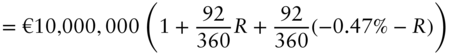

on September 15, which is exactly the same as if it had borrowed €10 million at a rate of ![]() 0.47%. Intuitively, if realized Euribor on June 15 is less than
0.47%. Intuitively, if realized Euribor on June 15 is less than ![]() 0.47%, the corporation borrows at relatively low rates, but owes money on the FRA. On the other hand, if realized Euribor is greater than
0.47%, the corporation borrows at relatively low rates, but owes money on the FRA. On the other hand, if realized Euribor is greater than ![]() 0.47%, the corporation borrows at relatively high rates but collects money on the FRA.9
0.47%, the corporation borrows at relatively high rates but collects money on the FRA.9
An exchange‐traded alternative to Euribor FRAs are Euribor futures contracts, some of which are listed in Table 12.10, as of January 14, 2022. The tickers begin with “ER,” followed by the month and year indicators. The contracts are subject to daily settlement, and the final settlement rate is set to three‐month Euribor on the last trade date. The final settlement rate of the June contract, for example, is three‐month Euribor on June 13, 2022, which as mentioned earlier, represents the rate on a loan from June 15 to September 15. Three‐month Euribor futures are scaled to hedge the change in interest on a €1 million, 90‐day loan. Equivalently, a one‐basis‐point change in rate translates into a daily settlement flow of €1,000,000 × 0.01% × 90/360, or €25.
The corporation in the FRA example hedges a €10 million, 92‐day loan from June 15 to September 15, 2022. This time period corresponds exactly to that covered by Euribor set on June 13, which is also the expiration of the June three‐month Euribor contract. Furthermore, with the market at the levels in Table 12.10 – a rate of ![]() 0.47% – the corporation can sell the June contract to lock in a rate of
0.47% – the corporation can sell the June contract to lock in a rate of ![]() 0.47% on its planned borrowing. The number of contracts required to hedge the €10 million, 92‐day loan with a contract scaled to a €1 million, 90‐day loan, is,
0.47% on its planned borrowing. The number of contracts required to hedge the €10 million, 92‐day loan with a contract scaled to a €1 million, 90‐day loan, is,

TABLE 12.10 Selected Three‐Month Euribor Futures Contracts, as of January 14, 2022. Rates Are in Percent.
| Delivery | Last Trade | |||
|---|---|---|---|---|
| Ticker | Month | Date | Price | Rate |
| ERH2 | Mar | 03/14/22 | 100.540 | −0.540 |
| ERM2 | Jun | 06/13/22 | 100.470 | −0.470 |
| ERU2 | Sep | 09/19/22 | 100.375 | −0.375 |
| ERZ2 | Dec | 12/19/22 | 100.260 | −0.260 |
TABLE 12.11 Hedging the Interest Cost of Borrowing €10 Million from June 15, 2022, to September 15, 2022, as of January 14, 2022, with June Three‐Month Euribor Contracts, Priced Initially at![]() 0.47%. The Hedge, Not Tailed, Sells 10.22 Contracts. Rates Are in Percent. Other Entries Are in Euro.
0.47%. The Hedge, Not Tailed, Sells 10.22 Contracts. Rates Are in Percent. Other Entries Are in Euro.
| Final Settlement Rate | Loan Interest | Futures P&L | Net |
|---|---|---|---|
| −0.77 | 19,677.78 | −7,665.00 | 12,012.78 |
| −0.47 | 12,011.11 | 0.00 | 12,011.11 |
| −0.17 | 4,344.44 | 7,665.00 | 12,009.44 |
The results of the hedge are given in Table 12.11. If rates rise, so that Euribor on June 13 turns out to be ![]() 0.17%, the corporation receives interest of €10 million × (92/360) × negative 0.17%, or €4,344.44; experiences a futures gain of 30 basis points per contract, for a total gain – ignoring the small effects of daily settlement – of 30 × €25 × 10.22, or €7,665.00; which together gives an overall gain of €12,009.44. Looking at the table as a whole, the futures position successfully hedges the cost of borrowing in the sense of locking in the receipt of about €12,011. The hedge would be exact if the number of contracts in Equation (12.16) were taken to more decimal places.
0.17%, the corporation receives interest of €10 million × (92/360) × negative 0.17%, or €4,344.44; experiences a futures gain of 30 basis points per contract, for a total gain – ignoring the small effects of daily settlement – of 30 × €25 × 10.22, or €7,665.00; which together gives an overall gain of €12,009.44. Looking at the table as a whole, the futures position successfully hedges the cost of borrowing in the sense of locking in the receipt of about €12,011. The hedge would be exact if the number of contracts in Equation (12.16) were taken to more decimal places.
This hedging example is simple in that the corporation plans to borrow over the same period as covered by three‐month Euribor relevant for the June contract. Along the same lines as the discussion in the context of hedging with SOFR futures, if the borrowing period were shorter or longer than that covered by the June Euribor contract, fewer or more contracts would be needed, and contracts other than June might be used.
The example in this section is constructed to show the similarity between Euribor FRAs and futures, but there are significant differences as well. FRAs may be subject to bilateral margin agreements, but are not subject to daily settlement, like futures. FRAs, as over‐the‐counter products, can be customized for individual trades with respect to dates covered and with respect to notional amount, while the terms of futures contracts are highly standardized. In part because they are customized, however, FRAs are less liquid than futures. Hedgers typically need to decide, therefore, whether customization or liquidity is more important in their particular circumstances.
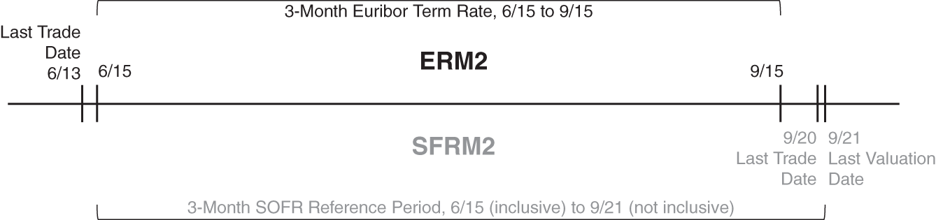
FIGURE 12.5 A Comparison of the June 2022 Euribor and the June 2022 SOFR Futures Contracts.
This section concludes with a comparison of futures on a forward‐looking term rate benchmark, like Euribor, and futures on a backward‐looking compounded overnight benchmark, like SOFR. The top half of Figure 12.5 depicts the June three‐month Euribor contract, ERM2, while the bottom half depicts the June three‐month SOFR contract, SFRM2. Both contracts cover realized interest rates from mid‐June to mid‐September, though the terminal date differs somewhat, as detailed earlier. The big difference, however, is that ERM2, which references a term rate set on June 13, expires on that date. SFRM2, which references a compounded daily rate that is not known until September 21, does not expire until that later date.
12.6 THE FUTURES‐FORWARD DIFFERENCE
By definition, borrowers and lenders can lock in market forward rates, and earlier sections of this chapter show that, ignoring daily settlement, borrowers and lenders can also lock in market futures rates. This section explains that, because of daily settlement, market futures rates exceed market forward rates. However, the magnitude of the difference turns out to be small except for contracts of the longest terms.
If a trader receives fixed at 2% through a forward agreement, all of the P&L from the agreement is realized at its expiration. But if the trader buys an otherwise identical futures contract at 2%, that same total P&L is realized over time. More specifically, when rates are falling and the futures contract is making money, daily settlement profits are reinvested at relatively low rates. And when rates are rising and the futures contract is losing money, daily settlement losses have to be financed at relatively high rates. Therefore, averaging across scenarios of both falling and rising rates, receiving daily settlement payments over time is worse than receiving all of the P&L at the end. Hence, traders require a higher rate when buying a futures contract than when receiving fixed in a forward agreement. Or, in reverse, other traders willingly accept a higher rate when selling a futures contract than when paying fixed in a forward agreement. In this example, the futures rate exceeds the forward rate of 2%. Furthermore, based on the logic of that result, the difference between the two rates increases with the length of time to expiration of the contracts and with the volatility of interest rates.
Appendix A12 proves, in general, that the futures rate exceeds the forward rate.10 For the purposes of understanding orders of magnitude, however, Table 12.12 presents some results, without proof, from a normal one‐factor term structure model with a constant drift and with a constant volatility of 80 basis points per year. This volatility is chosen to be roughly consistent with the levels shown in Chapter 16. In any case, the rows of the table in the first and second panels correspond to the three different kinds of futures contracts described in this chapter: three‐month contracts on a term rate (Euribor futures); one‐month contracts on an average of overnight rates (fed funds and SOFR futures); and three‐month contracts on compounded overnight rates. The first panel gives the formulas for the differences between futures and forward rates in the model just described, where ![]() denotes the annual normal volatility (e.g., 0.8% for 80 basis points);
denotes the annual normal volatility (e.g., 0.8% for 80 basis points); ![]() denotes the term of the underlying rate, in years, which, for the contracts shown, is either 0.25 or 1/12; and
denotes the term of the underlying rate, in years, which, for the contracts shown, is either 0.25 or 1/12; and ![]() denotes the time to the beginning of the rate reference period. As an illustration of
denotes the time to the beginning of the rate reference period. As an illustration of ![]() from the examples in the text, the beginning of the reference period of the three‐month June Euribor and three‐month June SOFR contracts depicted in Figure 12.5 – June 15 – is 152 days or about
from the examples in the text, the beginning of the reference period of the three‐month June Euribor and three‐month June SOFR contracts depicted in Figure 12.5 – June 15 – is 152 days or about ![]() years from the trade date of January 14.
years from the trade date of January 14.
TABLE 12.12 The Futures‐Forward Rate Difference for Selected Contracts in a One‐Factor Model with a Volatility of 80 Basis Points per Year.
| Underlying | Contract | ||||
|---|---|---|---|---|---|
| Rate | Examples | Formula | |||
| Term | 3m Euribor |  | 0.25 | ||
| Avg. ON | 1m FF/SOFR | 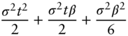 | |||
| Comp. ON | 3m SOFR | 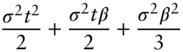 | 0.25 | ||
| Fut‐Fwd Difference (bps) | |||||
| t | t | t | t | ||
| Term | 3m Euribor | 0.4 | 1.4 | 8.4 | 32.8 |
| Avg. ON | 1m FF/SOFR | 0.3 | 1.3 | 8.1 | 32.3 |
| Comp. ON | 3m SOFR | 0.4 | 1.5 | 8.4 | 32.8 |
The second panel of Table 12.12 gives the differences between the futures and forward rates in the model for each of the contract types and for four values of ![]() , in basis points. The first point to notice is that futures‐forward rate differences for a given
, in basis points. The first point to notice is that futures‐forward rate differences for a given ![]() do not vary much across contracts. The reason for this can be seen from the formulas in the first panel. With
do not vary much across contracts. The reason for this can be seen from the formulas in the first panel. With ![]() relatively small, the dominant term in all the formulas is the common term
relatively small, the dominant term in all the formulas is the common term ![]() . The second point to notice is that the futures‐forward rate difference is relatively small except for the longest times to the beginning of the reference period. This is again explained by the dominant term,
. The second point to notice is that the futures‐forward rate difference is relatively small except for the longest times to the beginning of the reference period. This is again explained by the dominant term, ![]() , which increases with the square of
, which increases with the square of ![]() . That term alone, in fact, is a good approximation for all of the terms in the given formulas: for
. That term alone, in fact, is a good approximation for all of the terms in the given formulas: for ![]() , for example,
, for example, ![]() equals 32 basis points, which approximately equals the exact solution for all of the contract types.
equals 32 basis points, which approximately equals the exact solution for all of the contract types.
NOTES
- 1 Reuters (2012),“Insight: A Greek Banker, the Shah and the Birth of LIBOR,” August 7.
- 2 See, for example, Amor, J. (2021), “The New EURIBOR Gets Through a Challenging 2020,” Funcas SEFO 10(1), pp. 49‐61, January.
- 3 For example, the OCC (Office of the Comptroller of the Currency) noted that “While banks may use any replacement rate [for LIBOR] they determine to be appropriate for their funding model and customer needs, OCC supervisory efforts will initially focus on non‐SOFR rates.” OCC (2021), “LIBOR Transition: Updated Self‐Assessment Tool for Banks,” OCC Bulletin 2021‐46, October 18. And an executive vice president and general counsel at the Federal Reserve Bank of New York said that “If your firm is moving to a rate other than SOFR, that means extra work for you to make sure you're demonstrably making a responsible decision. Because you are going to be asked about that decision.” Held, M. (2021),“Prepare for Landing,” Remarks at the ISDA Benchmark Strategies Forum, Federal Reserve Bank of New York, September 15.
- 4 The minimum price increment and, therefore, the precision or number of decimal places in the price of each contract, depends on the day of the week of the first day in the settlement month and on the remaining time to contract expiration.
- 5 The Federal Reserve Bank of New York releases the SOFR of a given day on the morning of the next business day, which determines the earliest availability of the monthly average. February 28, 2022, for example, is a Monday, which means that the February average is available on March 1.
- 6 For more on the operations and risk management of the exchange and its associated clearinghouse, see Chapter 13.
- 7 For additional institutional details, see, for example, Craig, B., and Millington, S. (2017), “The Federal Funds Market Since the Financial Crisis,” Economic Commentary 2017–07, Federal Reserve Bank of Cleveland, April 5.
- 8 There is another way to back out rate expectations of the January meeting, namely, to match the January futures rate as an average of 26 days at eight basis points and five days at the expected result of the January meeting. The purpose of the text, however, is merely to illustrate the procedure, not to recommend a specific approach for this particular point in time.
- 9 The most creditworthy corporations might be able to borrow at Euribor flat, as in the example. Less creditworthy entities borrow at Euribor plus a spread, which, despite negative Euribor, might result in an overall positive interest payment. In any case, to the extent the bank can set the spread at the time of the loan, the corporation is exposed to spread risk.
- 10 This result is analogous to the result in Chapter 11 that the futures price is less than the forward price.