
CHAPTER 6
Regression Hedging and Principal Component Analysis
The risk metrics and hedges of Chapters 4 and 5 assume relationships across rates of different terms. The assumptions are typically motivated by a combination of economic theory, empirical analysis of historical data, and views about future economic and financial developments. This chapter introduces approaches that rely explicitly on historical data. It would be an oversimplification, however, to categorize the techniques of Chapters 4 and 5 as subjective, while categorizing the approaches of this chapter as objective. Empirical methods also require assumptions, such as the number of rates or instruments used in the analysis, the particular rates or instruments chosen, and the historical time period selected for estimation.
The first section of this chapter describes single‐variable regression hedging in the context of hedging a 40‐year Johnson & Johnson (JNJ) bond with a 30‐year Treasury. The second section describes two‐variable regression hedging in the context of a relative value trade of 20‐year versus 10‐ and 30‐year Treasuries. The third and fourth sections discuss two other issues that arise in the context of regression hedging, namely, the choice between level and change regressions, and reverse regressions.
One conceptual problem with using regression hedging in practice is that each regression is essentially a different model of the term structure of interest rates with different underlying assumptions. Consider, for example, the manager of a trading desk in which some traders are using single‐variable regressions and some two‐variable regressions, or some are estimating regressions from one month of historical data and others from six months.
The final section of the chapter introduces a unified empirical description of how the entire term structure evolves, namely, principal component analysis (PCA). PCA provides both an empirical hedging methodology, which can be used consistently across the term structure, along with easily interpreted descriptions of how the term structure fluctuates over time. While presentations of PCA tend to be highly mathematical, great effort has been made in this chapter to make the material more broadly accessible.
6.1 SINGLE‐VARIABLE REGRESSION HEDGING
This section considers the problem of a market maker or a relative value trader on May 14, 2021, who purchases $100 million face amount of the JNJ 2.450s of 09/01/2060 and hedges the resulting interest rate risk by selling the US Treasury 1.625s of 11/15/2050. Because there is no 40‐year Treasury bond outstanding, the 1.625s of 11/15/2050, with about 30 years to maturity, are selected as the best alternative. Table 6.1 gives the coupons, maturity dates, yields, and DV01s of these two bonds, along with those of two other bonds that are referenced in the next section.
The trader can choose the face amount of the Treasury bond in the hedge using the ratio of DV01s, along the lines of Chapter 4. In this case, the trader sells $100 million × ![]() , or $111.2 million. As discussed in Chapter 4, however, this hedge assumes that the yields of the JNJ and Treasury bonds move up or down in parallel. But because the JNJ bonds sell at a changing corporate spread to Treasuries, and because 40‐ and 30‐year rates are not perfectly correlated, as emphasized in Chapter 5, there is good reason to question the assumption of parallel yield shifts in this case.
, or $111.2 million. As discussed in Chapter 4, however, this hedge assumes that the yields of the JNJ and Treasury bonds move up or down in parallel. But because the JNJ bonds sell at a changing corporate spread to Treasuries, and because 40‐ and 30‐year rates are not perfectly correlated, as emphasized in Chapter 5, there is good reason to question the assumption of parallel yield shifts in this case.
The scatter plot in Figure 6.1 shows the daily changes in yield of the JNJ bonds against those of the Treasury bond from January 19, 2021, to May 14, 2021, which is a window of about four months before the date of the hedge. The line in the figure is the regression line fitted through the data, which is discussed presently. The figure teaches two lessons. First, there is a lot of variation in the relationship between these changes. Some days, the Treasury yield changes by more (e.g., the point on the graph at (![]() 18.2,
18.2, ![]() 11.1)); some days by less (e.g., the point (
11.1)); some days by less (e.g., the point (![]() 3.3,
3.3, ![]() 7.7)); and some days even in opposite directions (e.g., the point (2.0,
7.7)); and some days even in opposite directions (e.g., the point (2.0, ![]() 2.2)). Second, from the slope of the line, the average relationship between yield changes is less than one‐to‐one; that is, the change in the yield of the JNJ bonds tends to be less than the change in the yield of the Treasury bonds.
2.2)). Second, from the slope of the line, the average relationship between yield changes is less than one‐to‐one; that is, the change in the yield of the JNJ bonds tends to be less than the change in the yield of the Treasury bonds.
Figure 6.1 implicitly assumes that the most relevant period for designing an empirical hedge is the recent, immediate past. This assumption is often reasonable, but there are times and situations in which some earlier period seems more relevant. For example, if the Federal Reserve is expected to raise short‐term rates in the immediate future, a similar episode in the past might be more relevant to the future than the recent past, in which the Federal Reserve left rates unchanged or lowered them. Choosing the length of the observation or estimation window is also part of the art of regression hedging. Too short a window might fail to furnish statistically reliable estimates, but too long a window might include less relevant historical data.
TABLE 6.1 Yields and Yield‐Based DV01s for the JNJ 2.450s of 09/01/2060 and Selected US Treasury Bonds, as of May 14, 2021. Yields Are in Percent.
| Issuer | Bond | Yield | DV01 |
|---|---|---|---|
| JNJ | 2.450s of 09/01/2060 | 2.962 | 0.2124 |
| Treasury | 0.875s of 11/15/2030 | 1.601 | 0.0847 |
| Treasury | 1.375s of 11/15/2040 | 2.246 | 0.1446 |
| Treasury | 1.625s of 11/15/2050 | 2.364 | 0.1910 |
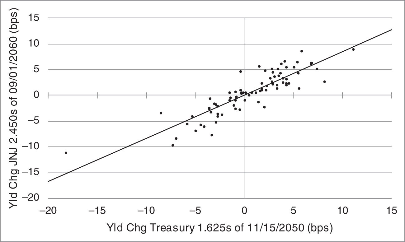
FIGURE 6.1 Regression of Daily Changes in Yields of the JNJ 2.450s of 09/01/2060 on Daily Changes in Yields of the Treasury 1.625s of 11/15/2050, from January 19, 2021, to May 14, 2021.
In light of the empirical evidence in Figure 6.1, the trader might very well choose to: i) adjust the hedge ratio to account for the less than one‐to‐one relationships between changes in yields; and ii) measure the variation around the average relationship to gain a better understanding of the risk of the hedged position. Regression analysis is a tool with which to achieve both of these objectives.
Let ![]() and
and ![]() be the changes in yields of the JNJ and 30‐year Treasury bonds on date
be the changes in yields of the JNJ and 30‐year Treasury bonds on date ![]() , respectively. A regression model linking these changes is,
, respectively. A regression model linking these changes is,
Equation (6.1) says that the dependent variable, here the change in the yield of the JNJ bond, equals: a constant or intercept, ![]() ; plus a slope,
; plus a slope, ![]() , times the independent variable, here the change in the yield of the 30‐year Treasury bond; plus an error term,
, times the independent variable, here the change in the yield of the 30‐year Treasury bond; plus an error term, ![]() . The unknown constant and slope parameters are estimated from the data, in a manner explained presently. These estimated parameters, denoted
. The unknown constant and slope parameters are estimated from the data, in a manner explained presently. These estimated parameters, denoted ![]() and
and ![]() , respectively, can then be used for prediction. Given the change in the Treasury bond yield on date
, respectively, can then be used for prediction. Given the change in the Treasury bond yield on date ![]() , the predicted change in the yield of the JNJ bonds on that date, denoted
, the predicted change in the yield of the JNJ bonds on that date, denoted ![]() , is,
, is,
and the realized error or residual on that day, ![]() , is given by,
, is given by,
For example, say that the estimated constant and slope parameters are 0 and 0.84, respectively, and that the Treasury bond yield changes by ![]() basis points. Then, by Equation (6.2), the predicted change in the yield of the JNJ bond is
basis points. Then, by Equation (6.2), the predicted change in the yield of the JNJ bond is ![]() basis points. If, furthermore, the actual change in the JNJ bond is
basis points. If, furthermore, the actual change in the JNJ bond is ![]() basis points, then, by (6.3) or (6.4), the realized error or residual is
basis points, then, by (6.3) or (6.4), the realized error or residual is ![]() or 4.2 basis points. In Figure 6.1, this residual can be thought of as a vertical line dropped from the data point, (
or 4.2 basis points. In Figure 6.1, this residual can be thought of as a vertical line dropped from the data point, (![]() 18.2,
18.2, ![]() 11.1), to the regression line.
11.1), to the regression line.
Least‐squares estimation of the unknown parameters finds ![]() and
and ![]() to minimize the sum of the squares of the residuals over the observation period,
to minimize the sum of the squares of the residuals over the observation period,
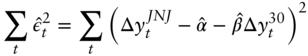
where the equality follows from Equation (6.3). Squaring of the errors ensures that offsetting positive and negative errors are not considered as acceptable as zero errors, and that large errors in absolute value are penalized heavily relative to smaller errors.
Least‐squares estimation assumes that the regression model is a true description of the dynamics of the dependent and independent variables, that the errors across time have the same probability distribution, that they are independent of each other, and that they are uncorrelated with the independent variable. Under these assumptions, least‐squares parameter estimates are linear, unbiased, consistent, and efficient.1
Least‐squares estimation is available in many statistical packages and spreadsheets. Table 6.2 gives a typical summary output from estimating Equation (6.1) using the data shown in Figure 6.1. The estimate of the slope coefficient, ![]() , is 0.842, which says that, on average, the change in the yield of the JNJ bond is only 0.842 times the change in the yield of the Treasury bond, which is very different from a parallel shift. The estimate of the constant,
, is 0.842, which says that, on average, the change in the yield of the JNJ bond is only 0.842 times the change in the yield of the Treasury bond, which is very different from a parallel shift. The estimate of the constant, ![]() is not very different from zero, which is typically the case in regressions of this sort. From an economic perspective, it would be odd if, over an extended period of time, changes in the yield of the JNJ bond tended to be positive or negative when there is no change in the yield of the Treasury bond. The line in Figure 6.1 is the fitted regression line, which is Equation (6.2) with its estimated coefficients,
is not very different from zero, which is typically the case in regressions of this sort. From an economic perspective, it would be odd if, over an extended period of time, changes in the yield of the JNJ bond tended to be positive or negative when there is no change in the yield of the Treasury bond. The line in Figure 6.1 is the fitted regression line, which is Equation (6.2) with its estimated coefficients,
Table 6.2 also gives the standard errors of the constant and slope coefficients, which provide confidence intervals around the estimates: the interval of each estimate plus or minus two standard errors falls around the true parameter values approximately 95% of the time. In this regression, the confidence intervals are 0.060 plus or minus 2 times 0.223, or ![]() , and 0.842 plus or minus 2 times 0.051, or
, and 0.842 plus or minus 2 times 0.051, or ![]() . Hence, because the confidence interval around the estimated constant includes zero, the hypothesis that
. Hence, because the confidence interval around the estimated constant includes zero, the hypothesis that ![]() cannot be rejected with 95% confidence. But, because the confidence interval for the slope coefficient does not include one, the hypothesis that
cannot be rejected with 95% confidence. But, because the confidence interval for the slope coefficient does not include one, the hypothesis that ![]() can be rejected with 95% confidence. Hence, the hypothesis of parallel shifts in the yields of the two bonds is rejected by the data.
can be rejected with 95% confidence. Hence, the hypothesis of parallel shifts in the yields of the two bonds is rejected by the data.
TABLE 6.2 Regression of Daily Changes in Yields of the JNJ 2.450s of 09/01/2060 on Daily Changes in Yields of the Treasury 1.625s of 11/15/2050, from January 29, 2021, to May 14, 2021.
| No. of Observations | 82 | |
|---|---|---|
| R‐Squared | 77.5% | |
| Standard Error | 2.00 | |
| Regression Coefficients | Value | Std. Error |
| Constant ( | 0.060 | 0.223 |
| Chg 30yr Treasury Yield ( | 0.842 | 0.051 |
Table 6.2 reports that the R‐squared of the regression is 77.5%, meaning that 77.5% of the variance of changes in the JNJ yield can be explained by the model, that is, by changes in the yield of the 30‐year Treasury bond. In a one‐variable regression, the R‐squared is just the square of the correlation between the dependent and independent variables, which gives a correlation here of ![]() , or 88.0%. That these statistics are well below 1.0 indicates that hedging in this case does not come close to eliminating all interest rate risk.
, or 88.0%. That these statistics are well below 1.0 indicates that hedging in this case does not come close to eliminating all interest rate risk.
The remaining statistic to be discussed in Table 6.2 is the standard error of the regression, which is essentially the standard deviation of the realized errors or residuals, as defined in Equations (6.3) and (6.4).2 This standard error is a measure of how well the model fits the data and is in the same units as the dependent variable, in this case, basis points. Roughly speaking, then, the standard deviation of the errors in explaining daily changes in the yield of the JNJ bond with daily changes in the yield of the Treasury bond is two basis points. This statistic is particularly useful in describing the risk of a regression‐based hedge, as discussed presently.
All the results in Table 6.2 are in‐sample; that is, they are computed from the particular data sample used to estimate the regression model. Relying on these results for hedging assumes that the future will be sufficiently like this particular historical period. The success or failure of this assumption is discussed at the end of the section.
Turning now to regression hedging, assume for the moment that the yield of the JNJ bonds changes by exactly ![]() basis points for every one‐basis‐point change in the yield of the Treasury bonds. Let
basis points for every one‐basis‐point change in the yield of the Treasury bonds. Let ![]() ,
, ![]() ,
, ![]() , and
, and ![]() be the face amounts and DV01s of the JNJ and 30‐year Treasury bonds, respectively. Then, the position is hedged against changes in yields if,
be the face amounts and DV01s of the JNJ and 30‐year Treasury bonds, respectively. Then, the position is hedged against changes in yields if,

Plugging in numbers, $100 million for the face amount of the JNJ bonds to be hedged, DV01s from Table 6.1, and ![]() from Table 6.2,
from Table 6.2,
The yield‐based DV01 hedge for the JNJ bonds, which is given by Equation (6.9), is given earlier without the slope coefficient of 0.842 as $111.2 million. The regression hedge of (6.9) sells only $93.6 million because it recognizes that the yield of the JNJ bonds does not move as much as the yield of the 30‐year Treasury bond. Hence, fewer Treasury bonds need be sold to hedge the interest rate risk of the JNJ bonds.
Regression hedges are sometimes described in terms of risk weights. Rearranging terms in Equation (6.7) or (6.8),
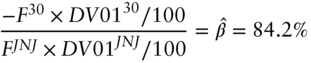
In words, the left‐hand side of the equation is the DV01 of the hedge as a fraction of the DV01 of the bonds being hedged. The risk weight of a yield‐based DV01 hedge is always 100% – the DV01s of the two sides of the trades are, by construction, equal. In this regression hedge, however, the DV01 of the Treasury bonds is only 84.2% of the DV01 of the JNJ bonds. In general, as Equation (6.10) shows, the risk weight of a regression hedge exactly equals the estimated slope coefficient, ![]() .
.
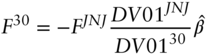
The best argument for the regression hedge is actually not the earlier assumption that bond yields change exactly according to the regression model. Write the P&L of the position as,
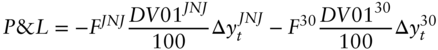
where the negative signs reflect that a positive face amount with a positive change (i.e., increase) in yield lowers P&L. It can then be shown that the regression hedge in Equation (6.8) minimizes the variance (6.11). (See Appendix A6.1.) In other words, to the extent that P&L variance is an appropriate measure of risk, the regression hedge minimizes the risk of the hedged position.
Appendix A6.1 also derives the standard deviation of the regression‐hedged P&L. Denote this standard deviation by ![]() and the standard deviation of the residuals by
and the standard deviation of the residuals by ![]() . Then,
. Then,

where ![]() is the symbol for absolute value, so that the standard deviation is positive whether the original position is long (positive
is the symbol for absolute value, so that the standard deviation is positive whether the original position is long (positive ![]() ) or short (negative
) or short (negative ![]() ). In words, the P&L of the hedged position is the DV01 of the position being hedged times the standard error of the regression residuals. Intuitively, the hedged P&L on any given day is exactly zero if the yield of the JNJ bonds moves by 0.842 basis points times the change in the Treasury yield. But if the residual is one basis point, so that the yield of the JNJ bond increases by one basis point more than that, the hedged position loses the DV01 of the JNJ bonds; and if the residual is minus two basis points, then the hedged position gains twice the DV01 of the JNJ bonds; etc. Hence, the volatility of the hedge is proportional to the variability of the residuals.
). In words, the P&L of the hedged position is the DV01 of the position being hedged times the standard error of the regression residuals. Intuitively, the hedged P&L on any given day is exactly zero if the yield of the JNJ bonds moves by 0.842 basis points times the change in the Treasury yield. But if the residual is one basis point, so that the yield of the JNJ bond increases by one basis point more than that, the hedged position loses the DV01 of the JNJ bonds; and if the residual is minus two basis points, then the hedged position gains twice the DV01 of the JNJ bonds; etc. Hence, the volatility of the hedge is proportional to the variability of the residuals.
Applying Equation (6.12) to the case at hand, the DV01 of the JNJ bond position is $100 million × ![]() , or $212,400, and the standard error of the regression, reported in Table 6.2, is two basis points per day. Therefore, the standard deviation of the hedged P&L in the sample is $212,400 × 2 or $424,800 per day. Whether this is too much risk or not depends on how much and how fast the trader is making money buying the JNJ bonds and hedging them. If the trader is making five basis points on the position and holding it for a day, then a standard deviation of two basis points per day likely represents a reasonable risk–return trade‐off. If, on the other hand, the trader is making 1.5 basis points and holding the position for a week, a standard deviation of two basis points per day likely ruins the trade from a risk–return perspective.
, or $212,400, and the standard error of the regression, reported in Table 6.2, is two basis points per day. Therefore, the standard deviation of the hedged P&L in the sample is $212,400 × 2 or $424,800 per day. Whether this is too much risk or not depends on how much and how fast the trader is making money buying the JNJ bonds and hedging them. If the trader is making five basis points on the position and holding it for a day, then a standard deviation of two basis points per day likely represents a reasonable risk–return trade‐off. If, on the other hand, the trader is making 1.5 basis points and holding the position for a week, a standard deviation of two basis points per day likely ruins the trade from a risk–return perspective.
This section concludes with an out‐of‐sample analysis of the estimated regression model. Figure 6.2 shows the same regression line as estimated in Table 6.2 and graphed in Figure 6.1. The plus signs, however, are the changes in yields over the period May 17, 2021, to July 19, 2021. The regression model, estimated over the earlier period, January 29, 2021, to May 15, 2021, holds up quite well. In fact, the standard error of the residuals of the out‐of‐sample data against the original regression line is 1.5 basis points, which is actually smaller than the in‐sample equivalent. The trader hedging as of May 14, 2021, cannot, of course, run this analysis. But other out‐of‐sample tests can be informative. A trader might see how a regression model performed over a period before the estimation period, perhaps a period right before that window or perhaps an even earlier period that might be more likely to resemble the future. In any case, poor out‐of‐sample performance should raise questions about the stability of the regression coefficients over time and, therefore, the reliability of the resulting hedge.
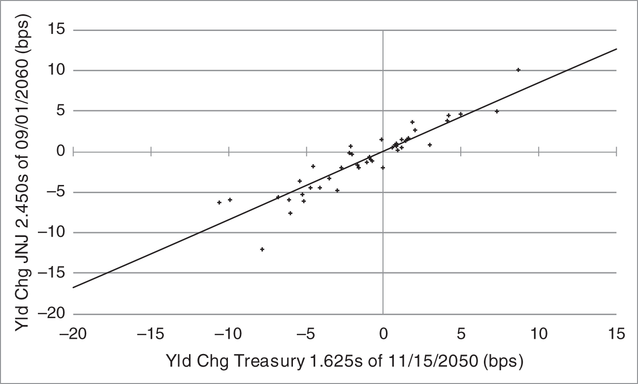
FIGURE 6.2 Yield Changes of the JNJ 2.450s of 09/01/2060 and the Treasury 1.625s of 11/15/2050 from May 17, 2021, to July 19, 2021, and the Regression Line Estimated over the Period January 19, 2021, to May 14, 2021.
6.2 TWO‐VARIABLE REGRESSION HEDGING
The hedging approaches of Chapter 5 generalize those of Chapter 4 to account for the fact that rates across the term structure are not perfectly correlated. Similarly, two‐variable regression hedges account for the fact that changes in a bond's yield might be better explained by changes in the yields of two other bonds, rather than just one, as in a one‐variable regression.
To illustrate two‐variable regression hedging, consider a relative value trader who believes that yields in the 20‐year US Treasury bond sector are too high – or prices too low – relative to the 10‐ and 30‐year sectors. Implementing this trade idea by buying a 20‐year bond outright is too risky: if rates increase across the board, the trade loses money even if the trader is right, that is, even if the 20‐year bond does outperform 10‐ and 30‐year bonds. But buying a 20‐year bond and hedging the interest rate risk by selling a 10‐year bond also bears too much risk that is unrelated to the trade idea: if the curve steepens (e.g., 30‐year yields increase more than 20‐year yields, which increase more than 10‐year yields), the trade may lose money even if the 20‐year bonds outperform. And, finally, buying a 20‐year bond and hedging with a 30‐year bond can lose money if the curve flattens even if the 20‐year bonds outperform. In practice then, this trade idea is typically implemented with a butterfly: buy 20‐year bonds and sell both 10‐ and 30‐year bonds: both shorts defend against general rate increases; the 10‐year short defends against flattening; and the 30‐year short defends against steepening. The trader's problem then becomes to choose the face amount of the 10‐ and 30‐year bonds to sell against, say, $100 million face amount of the 20‐year bond.
In this illustration, the trader chooses the three Treasury bonds listed in Table 6.1: the 1.375s of 11/15/2040 as the 20‐year; the 0.875s of 11/15/2030 as the 10‐year; and the 1.625s of 11/15/2050 as the 30‐year. The two‐variable regression model of changes in yields of these bonds is,
where the notation is analogous to that of the one‐variable regression. Here there are two slope coefficients, describing how changes in the 20‐year yield are related to changes in each of the 10‐year and 30‐year yields.
Continuing as in the case of one‐variable regression, least‐squares estimation finds the regression coefficients so as to minimize the sum of the squared residuals,
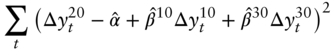
And, with these estimated coefficients, the predicted change of the 20‐year rate is,
Table 6.3 gives the results of the regression, estimated with data from January 29, 2021, to May 14, 2021. The R‐squared is quite high relative to that of the single‐variable regression, in Table 6.2, in part because two explanatory variables are used, rather than one, and in part because all of the bonds in this regression are Treasuries, whereas the single‐variable regression mixes a corporate bond with a Treasury bond. The standard error is also significantly lower here, at 1.15 basis points per day. Again, however, as usual for regressions of this sort, the estimate of ![]() is small and not significantly different from zero.
is small and not significantly different from zero.
The slope coefficients say that a one‐basis‐point increase in the 10‐year yield increases the 20‐year yield by 0.465 basis points, while a one‐basis‐point increase in the 30‐year yield increases the 20‐year yield by 0.669 basis points. With 95% confidence intervals for these coefficients of (0.329, 0.601) and (0.535, 0.803), respectively, both coefficients are significantly different from zero; that is, changes in the yields of both bonds are useful in explaining changes in the yield of the 20‐year bond.
TABLE 6.3 Regression of Daily Changes in Yields of the Treasury 1.375s of 11/15/2040 on Daily Changes in Yields of the Treasury 0.875s of 11/15/2030 and 1.625s of 11/15/2050, from January 29, 2021, to May 14, 2021.
| No. of Observations | 82 | |
|---|---|---|
| R‐Squared | 94.7% | |
| Standard Error | 1.15 | |
| Regression Coefficients | Value | Std. Error |
| Constant ( | 0.019 | 0.129 |
| Chg 10yr Treasury Yield ( | 0.465 | 0.068 |
| Chg 30yr Treasury Yield ( | 0.669 | 0.067 |
To derive the hedge based on these regression results, write the P&L of the hedged position as,

and then substitute for ![]() from (6.15) to see that,
from (6.15) to see that,
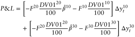
Next, to ensure that P&L is zero, under the assumption that the change in the 20‐year rate follows the regression model, set each of the terms in brackets in Equation (6.17) equal to zero. Solving,
or, in terms of risk weights,
Assuming a trade size of $100 million face amount in the 20‐year Treasury, substituting the DV01s of the bonds from Table 6.1 and the results of the regression from Table 6.3, the hedging face amounts and risk weights are $79.44 million and 46.5% for the 10‐year, along with $50.69 million and 66.9% for the 30‐year. Note that the sum of the risk weights is 113.4%, which means that the DV01 of the hedging position is 13.4% greater than the DV01 of the position being hedged. This follows immediately from the slope coefficients of the regression: a simultaneous one‐basis‐point change in both the 10‐ and 30‐year yields is associated with a 1.134‐basis‐point increase in the 20‐year yield. Hence, the hedging portfolio requires an extra 13.4% in DV01.
Figure 6.3 compares in‐sample and out‐of‐sample residuals from the regression in Table 6.3. The out‐of‐sample residuals are very well behaved, in fact, better behaved than the in‐sample residuals: the standard error is 1.15 in‐sample, and only 0.70 out‐of‐sample. Traders are not always so fortunate!
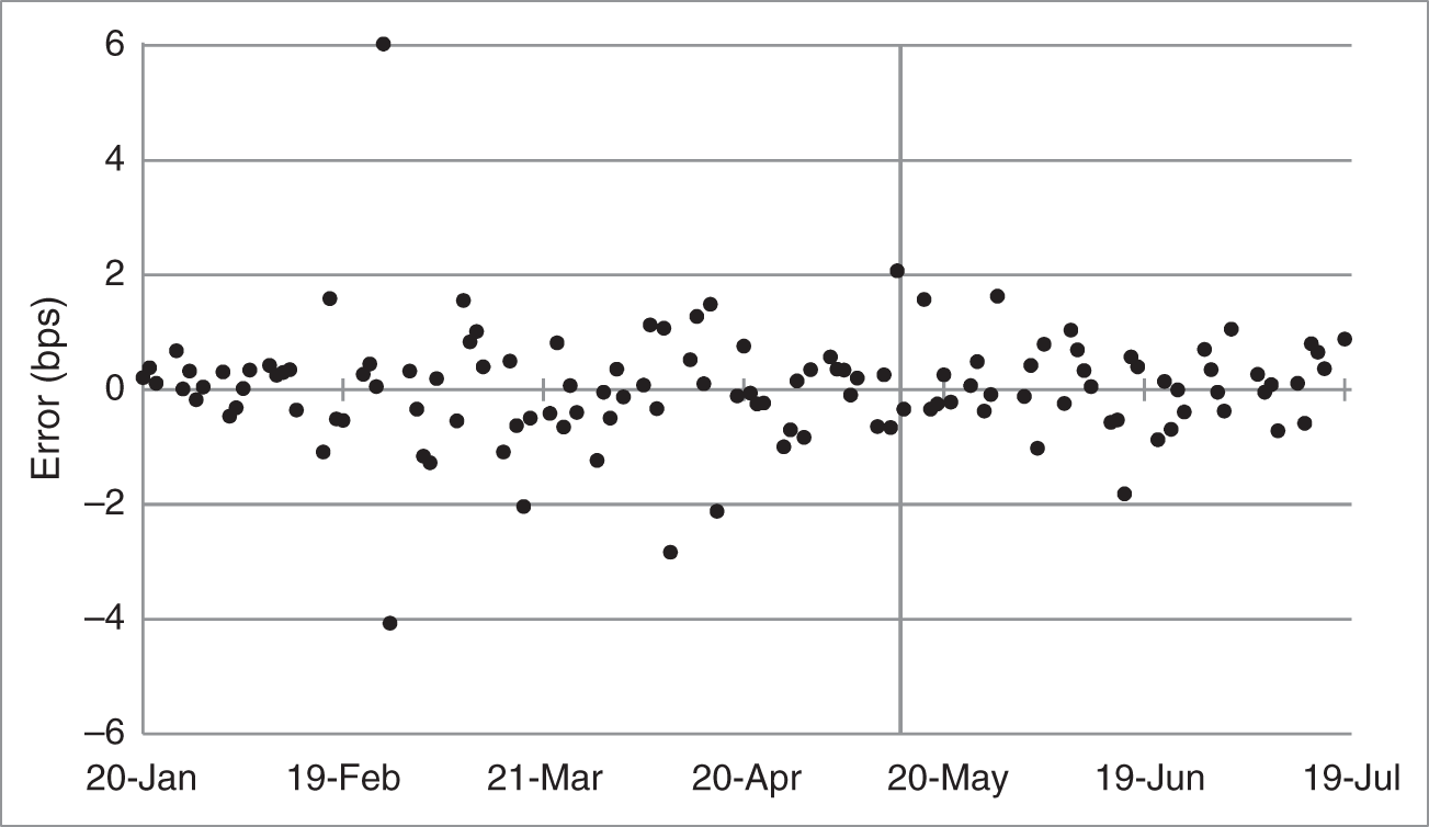
FIGURE 6.3 Residuals Using the Regression Coefficients in Table 6.3, in‐Sample – from January 19, 2021, to May 14, 2021 – and Out‐of‐Sample – from May 17, 2021, to July 19, 2021.
6.3 LEVEL VERSUS CHANGE REGRESSIONS
When estimating regression‐based hedges, most practitioners regress changes in yields on changes in yields, as in the previous sections, but some regress yields on yields. Mathematically, in the single‐variable case, the level‐on‐level regression with dependent variable ![]() and independent variable
and independent variable ![]() is,
is,
while the change‐on‐change regression is,3
If the assumptions of least‐squares estimation, mentioned earlier, hold true for the level model (6.22), then they also hold for the change model (6.24), and least‐squares estimates from both specifications are unbiased, consistent, and efficient. If, however, the assumption about the independence of the error terms is violated in either specification, then the least‐squares estimates from that specification may not be efficient, but they are still unbiased and consistent.
To discuss the economics behind the assumption that error terms are independent, say that ![]() , that
, that ![]() , and that
, and that ![]() and
and ![]() are the yields of two different bonds. Say further that the yield of the
are the yields of two different bonds. Say further that the yield of the ![]() ‐bond is constant at 5%, while the yield of the
‐bond is constant at 5%, while the yield of the ![]() ‐bond was 1% yesterday. The level regression, in Equation (6.22), predicts that the yield of the
‐bond was 1% yesterday. The level regression, in Equation (6.22), predicts that the yield of the ![]() ‐bond will be 5% today, despite its having been 1% yesterday. It is more likely, however, that the yield of the
‐bond will be 5% today, despite its having been 1% yesterday. It is more likely, however, that the yield of the ![]() ‐bond today will be closer to 1% than to 5%, and that the model error today will be closer to its value yesterday, of
‐bond today will be closer to 1% than to 5%, and that the model error today will be closer to its value yesterday, of ![]() 4%, than to zero. In other words, the error terms of the level regression are not likely to be independent of each other, but rather persistent, correlated over time, or serially correlated.
4%, than to zero. In other words, the error terms of the level regression are not likely to be independent of each other, but rather persistent, correlated over time, or serially correlated.
In this same scenario, because the change in the yield of the ![]() ‐bond is zero, the change‐on‐change regression in Equation (6.24) predicts that the change in the yield of the
‐bond is zero, the change‐on‐change regression in Equation (6.24) predicts that the change in the yield of the ![]() ‐bond is zero as well and that its yield remains at 1%. While more plausible than the level‐on‐level prediction that the yield of the
‐bond is zero as well and that its yield remains at 1%. While more plausible than the level‐on‐level prediction that the yield of the ![]() ‐bond suddenly jumps to 5%, it is more likely that the yield of the
‐bond suddenly jumps to 5%, it is more likely that the yield of the ![]() ‐bond will gradually trend from its current value of 1% to its model value of 5%. Hence, the error terms in the change‐on‐change regression are likely to be positive for some time, and, as such, serially correlated.
‐bond will gradually trend from its current value of 1% to its model value of 5%. Hence, the error terms in the change‐on‐change regression are likely to be positive for some time, and, as such, serially correlated.
This discussion suggests an alternate model, which would capture, in the scenario just discussed, that the yield of the ![]() ‐bond moves gradually from 1% to 5%. In particular, assume the level‐on‐level model, but with error dynamics,
‐bond moves gradually from 1% to 5%. In particular, assume the level‐on‐level model, but with error dynamics,
for some ![]() . In this model, with say,
. In this model, with say, ![]() , yesterday's error of
, yesterday's error of ![]() 4% would fall, on average, to an error of 75% times
4% would fall, on average, to an error of 75% times ![]() 4%, or
4%, or ![]() 3% today, thus giving an expected
3% today, thus giving an expected ![]() ‐bond yield today of 2%. In this way, the error structure in Equation (6.25) gradually pushes the yield of the
‐bond yield today of 2%. In this way, the error structure in Equation (6.25) gradually pushes the yield of the ![]() ‐bond up from its starting point of 1% to its model value, that is, the 5% yield of the
‐bond up from its starting point of 1% to its model value, that is, the 5% yield of the ![]() ‐bond. The procedure for estimating (6.22) with the error structure in (6.25) is given in many statistical texts.
‐bond. The procedure for estimating (6.22) with the error structure in (6.25) is given in many statistical texts.
6.4 REVERSE REGRESSIONS
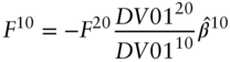
In Section 6.1, a trader regresses changes in yields of the JNJ 2.450s of 09/01/2060 – with a DV01 of 0.2124 – on changes in yields of the Treasury 1.625s of 11/15/2050 – with a DV01 of 0.1910; obtains a regression coefficient of 0.842; and, against $100 million of the JNJ bonds, calculates a regression hedge to sell $100 million × ![]() × 0.842, or $93.6 million Treasury bonds.
× 0.842, or $93.6 million Treasury bonds.
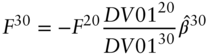
What if another trader runs the reverse regression, that is, regresses changes in yield of the Treasury bond on changes in yield of the JNJ bond? Table 6.4 compares the slope coefficients and standard errors of the original regression and the reverse regression. With a reverse regression ![]() of 0.921, this second trader hedges $93.6 million Treasury bonds with $93.6 million ×
of 0.921, this second trader hedges $93.6 million Treasury bonds with $93.6 million × ![]() × 0.921, or $82.8 million JNJ bonds.
× 0.921, or $82.8 million JNJ bonds.
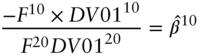
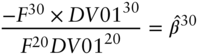
These hedges are clearly different. The same $93.6 million of Treasuries are hedged with a different amount of JNJ bonds. Or, in terms of risk weights, both quoted as the DV01 of the Treasury bond position as a percent of the DV01 of the JNJ position, the risk weight of the regression is 84.2%, while the risk weight of the reverse regression is ![]() , or 108.6%. Is one of these hedges right and the other wrong?
, or 108.6%. Is one of these hedges right and the other wrong?
This question actually reveals the importance of the trader's decision in Section 6.1 to hedge $100 million face amount of JNJ bonds. Choosing this face amount actually sets the risk of the trade. As shown earlier, the volatility of the hedged position is $100 million × ![]() × the two‐basis‐point standard error of the regression, or about $425,000. However, the risk of the reverse regression, which sets the face amount of the Treasury bonds at $93.6 million, is $93.6 million ×
× the two‐basis‐point standard error of the regression, or about $425,000. However, the risk of the reverse regression, which sets the face amount of the Treasury bonds at $93.6 million, is $93.6 million × ![]() × the 2.09 standard error of the reverse regression, or about $374,000. These trades, therefore, are not comparable.
× the 2.09 standard error of the reverse regression, or about $374,000. These trades, therefore, are not comparable.
Choosing to hedge $100 million face amount of the JNJ bonds, however, is not just about the risk of the hedged position. There are many combinations of positions in the JNJ and Treasury bonds that have the same volatility.4 For example, a scaled‐up reverse regression hedge, with $106.37 million Treasury bonds and $88 million JNJ bonds (i.e., $106.37 million × ![]() × 0.921), has the same $425,000 volatility as the regression hedge ($106.37 million ×
× 0.921), has the same $425,000 volatility as the regression hedge ($106.37 million × ![]() × 2.09). But while this and other positions might have the same volatility, because they do not hold $100 million in JNJ bonds, they are different trades. Most obviously, they do not satisfy the objective of buying $100 million of JNJ bonds from a client. Less obviously, to the extent that the return profile of the JNJ and Treasury bonds differ, different portfolios of the two bonds have different return characteristics as well.
× 2.09). But while this and other positions might have the same volatility, because they do not hold $100 million in JNJ bonds, they are different trades. Most obviously, they do not satisfy the objective of buying $100 million of JNJ bonds from a client. Less obviously, to the extent that the return profile of the JNJ and Treasury bonds differ, different portfolios of the two bonds have different return characteristics as well.
TABLE 6.4 Regression: Daily Changes in Yields of the JNJ 2.450s of 09/01/2060 on Daily Changes in Yields of the Treasury 1.625s of 11/15/2050. Reverse Regression: Daily Changes in Yields of the Treasury 1.625s of 11/15/2050 on Daily Changes in Yields of the JNJ 2.450s of 09/01/2060. Observations Are from January 29, 2021, to May 14, 2021.
| Regression | Reverse Regression | |
|---|---|---|
| 0.842 | 0.921 | |
| Standard Error | 2.00 | 2.09 |
In short, the regression hedge in Section 6.1 minimizes the variance of hedging $100 million face amount of the JNJ bonds. Trades with other objectives, like holding a fixed amount of Treasuries or holding a fixed amount of volatility risk with particular return characteristics, are constructed differently.
6.5 PRINCIPAL COMPONENT ANALYSIS
As mentioned in the introduction to this chapter, regression hedging tends to be ad hoc, because the relevant bonds and estimation periods are chosen separately for each application. Principal component analysis is useful, by contrast, in providing a single, empirical description of the behavior of the term structure that can be applied across a portfolio of fixed income instruments.
To illustrate PCA, this section uses daily data on fixed versus three‐month US Dollar (USD) LIBOR swap rates from June 1, 2020, to July 16, 2021.5 The data set consists of 13 times series, one for each of the terms from one to 10 years, as well as three with terms of 15, 20, and 30 years. These data can be summarized by the variances or standard deviations of changes in each rate and with their pairwise covariances or correlations. Another way to describe the data, however, is with 13 interest rate factors or components, where each factor represents a particular pattern of changes across the 13 rates. One factor, for example, might represent a simultaneous change of 0.2 basis points in the one‐year rate, 0.6 basis points in the two‐year rate, 1.2 basis points in the three‐year rate, etc., up to 3.7 basis points in the 20‐year rate, and 3.8 basis points in the 30‐year rate. PCA is a way to construct 13 factors, or principal components (PCs), such that they have the following properties:
- The sum of the variances of the PCs equals the sum of the variances of the individual rates. In this sense, the PCs capture the volatility of the set of interest rates.
- The PCs are uncorrelated with each other. While changes in rates of one term are highly correlated with changes in rates of another term, the PCs are constructed so that they are uncorrelated.
- Subject to (1) and (2), each PC is chosen to have the maximum possible variance given all earlier PCs. Therefore, the first PC explains the largest fraction of the sum of the variances of the rates; the second PC explains the next largest fraction; and so forth.
PCs of rates are particularly useful because of an empirical regularity: the sum of the variances of the first three PCs is usually an overwhelming fraction of the sum of the variances across all rates. Therefore, the variances and covariances of all rates are not necessary to describe how the term structure fluctuates: the structure and volatilities of only three PCs suffice. In the simplified context of three rates, Appendix A6.2 describes the construction of PCs in more detail. The text continues with a discussion of computed PCs for USD LIBOR swaps from the data set described earlier.
Figure 6.4 graphs the first three principal components, while Table 6.5 provides similar information in tabular form. Columns (2) to (4) correspond to the three PC curves in the figure, which can be interpreted as follows. A one standard deviation increase in the “level” PC, given both in Column (2) and the solid line in the figure, is a simultaneous increase in the one‐year rate of 0.23 basis points; in the two‐year rate of 0.59 basis points; in the 10‐year rate of 3.44 basis points; and in the 30‐year rate of 3.77 basis points. On a particular day, the change in the term structure might be best explained as a 1.5 standard deviation move in the first PC, that is, as adding 1.5 times each element of the first PC to corresponding swap rates. On another day, the change in the term structure might best be described as a ![]() 0.75 standard deviation move in the first component, that is, as subtracting 0.75 times each element of the first PC from current rates. In any case, the first PC has been traditionally called the “level” component because it has typically represented an approximately parallel shift over much of its range. In the empirical results presented here, however, the component is not particularly level for terms from one to seven years.
0.75 standard deviation move in the first component, that is, as subtracting 0.75 times each element of the first PC from current rates. In any case, the first PC has been traditionally called the “level” component because it has typically represented an approximately parallel shift over much of its range. In the empirical results presented here, however, the component is not particularly level for terms from one to seven years.
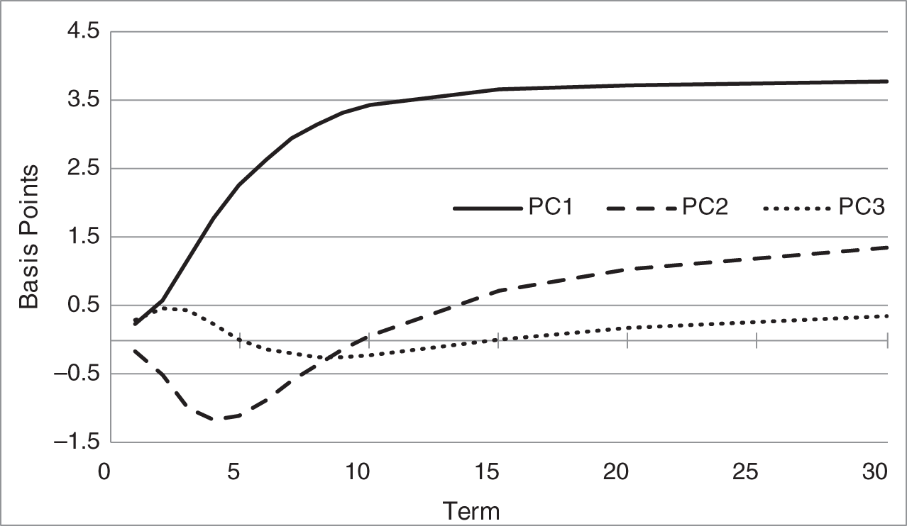
FIGURE 6.4 The First Three Principal Components of USD LIBOR Swap Rates, Estimated from June 1, 2020, to July 16, 2021.
TABLE 6.5 Principal Component Analysis of USD LIBOR Swap Rates from June 1, 2020, to July 16, 2021. Columns (2)‐(6) Are in Basis Points; Columns (7)‐(10) Are in Percent.
| (1) | (2) | (3) | (4) | (5) | (6) | (7) | (8) | (9) | (10) |
|---|---|---|---|---|---|---|---|---|---|
| PCs | % of PC Variance | ||||||||
| Short | PC | Total | Short | (5)/ | |||||
| Term | Level | Slope | Rate | Vol | Vol | Level | Slope | Rate | (6) |
| 1 | 0.23 | −0.16 | 0.29 | 0.41 | 0.55 | 32.7 | 15.0 | 52.3 | 74.54 |
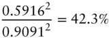
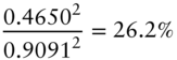
| 2 | 0.59 | −0.51 | 0.47 | 0.91 | 0.93 | 42.3 | 31.5 | 26.2 | 97.47 |
| 3 | 1.18 | −0.99 | 0.42 | 1.59 | 1.60 | 54.5 | 38.5 | 7.0 | 99.63 |
| 4 | 1.77 | −1.16 | 0.23 | 2.13 | 2.13 | 69.1 | 29.7 | 1.2 | 99.72 |
| 5 | 2.28 | −1.12 | 0.02 | 2.54 | 2.54 | 80.6 | 19.4 | 0.0 | 99.78 |
| 6 | 2.64 | −0.89 | −0.13 | 2.79 | 2.79 | 89.7 | 10.1 | 0.2 | 99.91 |
| 7 | 2.94 | −0.60 | −0.20 | 3.01 | 3.01 | 95.6 | 4.0 | 0.4 | 99.97 |
| 8 | 3.14 | −0.36 | −0.24 | 3.17 | 3.17 | 98.2 | 1.3 | 0.6 | 99.96 |
| 9 | 3.31 | −0.13 | −0.25 | 3.32 | 3.32 | 99.3 | 0.2 | 0.6 | 99.92 |
| 10 | 3.44 | 0.07 | −0.23 | 3.44 | 3.45 | 99.5 | 0.0 | 0.4 | 99.87 |
| 15 | 3.65 | 0.71 | 0.00 | 3.72 | 3.72 | 96.3 | 3.7 | 0.0 | 99.98 |
| 20 | 3.73 | 1.02 | 0.17 | 3.87 | 3.87 | 92.8 | 7.0 | 0.2 | 99.98 |
| 30 | 3.77 | 1.35 | 0.36 | 4.02 | 4.02 | 87.9 | 11.3 | 0.8 | 99.93 |
| Total | 9.99 | 2.92 | 0.96 | 10.45 | 10.47 | 91.3 | 7.8 | 0.8 | 99.84 |
A one standard deviation increase in the “slope” PC, given both in Column (3) of the table and the dashed line in the figure, is a simultaneous fall in the one‐year rate of 0.16 basis points; a fall in the two‐year rate of 0.51 basis points; an increase in the 10‐year rate of 0.07 basis points; and an increase in the 30‐year rate of 1.35 basis points. This PC is said to represent a “slope” change in rates because shorter‐term rates fall while longer‐term rates increase, or vice versa.
Lastly, a one standard deviation increase in the “short‐rate” PC, given both in Column (4) of the table and the dotted line in the figure, is a simultaneous small increase of very short‐term rates; a small decrease in intermediate‐term rates, and a small increase in long‐term rates. Because of its shape across terms, this PC is often named “curvature” as well, but, in light of the full discussion in this section, this PC is particularly useful for adding explanatory power to variations in shorter‐term rates.
To reiterate the sense in which the PCs describe changes in the term structure, on a given day, changes across terms might be described – picking numbers at random – as the combination of: a +1.5 standard deviation change in the first PC; a ![]() 0.4 standard deviation change in the second PC; and a
0.4 standard deviation change in the second PC; and a ![]() 1.8 standard deviation change in the third PC. The term structure at the end of that day, therefore, would approximately equal the term structure at the end of the previous day plus the contributions from the multiples of each of the three PCs. In this way, as explained shortly, these three PCs can indeed explain an overwhelmingly large proportion of realized term structure volatility.
1.8 standard deviation change in the third PC. The term structure at the end of that day, therefore, would approximately equal the term structure at the end of the previous day plus the contributions from the multiples of each of the three PCs. In this way, as explained shortly, these three PCs can indeed explain an overwhelmingly large proportion of realized term structure volatility.
The small values of the PCs at very short‐term rates reflect the low volatility of these rates. In the current financial environment, with the Federal Reserve promising to keep short‐term rates low for an extended period of time, current economic shocks are not envisioned as impacting short‐term rates until some time in the future. As a result, economic volatility is not reflected in very short‐term rates but seeps gradually into intermediate‐ and longer‐term rates as expectations of reactions to future Federal Reserve policy actions.6
Column (5) of Table 6.5 gives the combined standard deviation or volatility from the three principal components for each rate, while Column (6) gives the total, empirical volatility of each rate over the sample period. For the five‐year rate, for example, recalling that PCs are, by construction, uncorrelated, the volatility from the three PCs is,
The total volatility of the five‐year rate in the sample is also, to two decimal places, 2.54, but Column (10) – using more decimal places than shown in Columns (5) and (6) – reports that the ratio of five‐year PC volatility to total volatility is 99.78%. Hence, the empirical variation of the five‐year rate is almost completely explained by the first three PCs. Considering Column (10) as a whole, three PCs explain over 99% of the variation of rates of all terms greater than three years, 97.47% of the variation in the two‐year rate, and 74.54% of the variation in the one‐year rate. Hence, although there are 13 rates in the data series, three factors alone – three fixed combinations of changes in rates across terms – go a very long way in explaining the variation in all 13 rates. This is possible, intuitively, because changes in rates across terms are highly correlated; that is, nowhere near 13 factors are actually necessary to explain the variation in 13 rates. The performance of the three factors is less impressive, however, for rates of the shortest term.
Columns (7) through (9) of Table 6.5 give the variance explained by each of the first three PCs as a fraction of the total variance explained by those three PCs. For the two‐year rate, for example, those fractions are calculated as follows,

Note that, to avoid confusion, the values in these equations are reported to greater accuracy than those in the table.
Looking at Columns (7) to (9) across terms, the level PC dominates the other two as the main contributor to variations in the term structure. The short‐rate PC, and then the slope PC, are significant contributors at the short end, however, as is the slope PC for the longest rates. These finding have significant implications for risk management. A trader of eight‐ to 10‐year swaps, or perhaps even seven‐ to 15‐year swaps, can defend using the one‐factor metrics and hedging approaches of Chapter 4 and one‐variable regression hedging described in this chapter: according to Table 6.5, in this range of terms, term structure variation can be well described by a one‐factor model, like the level PC. On the other hand, traders in the three‐ to six‐year sector or the long end might very well require two factors, while traders in the very short end may not be comfortable without a three‐factor framework.
The last row of Table 6.5 computes the various statistics just discussed across the whole term structure of rates. More specifically, Columns (2) to (6) give the square root of the sum of variances across terms, and Columns (7) to (9) give the respective ratios for these totals. While the sum of variances is not a particularly interesting economic quantity – it does not represent the variance of any particularly interesting portfolio – the last row of the table does summarize two overall results of the PCA. First, 99.84% of the volatility of the 13 rates in the study is explained by the first three PCs. Second, the level PC explains over 90% of that variance, the slope PC about 8%, and the short‐rate PC less than 1%.
The overall lessons from PCA are often similar across global markets. Estimated over the same time period as the USD PCs in Figure 6.4, Figures 6.5 and 6.6 graph the first three PCs of British Pound Sterling (GBP) LIBOR and Euribor swap rates, respectively.7 The GBP PCs are extremely similar to their USD equivalents, with respect to both shape and magnitude. The biggest difference seems to be that the slope PC in USD is more volatile. The shapes of the EUR PCs are qualitatively similar to those in USD and GBP, but volatility in EUR is significantly lower. The EUR level PC, for example, flattens in the long end at a bit above 2.5 basis points per day, whereas the USD and GBP level PCs flatten at over 3.5. This lower volatility might be explained by the current aggressiveness of the European Central Bank, relative to the Federal Reserve and the Bank of England, to keep short‐term rates low over an extended period of time.
Hedges based on PCA are constructed like the multi‐factor approaches of Chapter 5. Using the current term structure, calculate the current price of the portfolio being hedged; shift the current term structure by each PC, in turn, to get new term structures and new portfolio prices; with these new prices, calculate a portfolio '01 with respect to each PC; and find a portfolio of hedging securities that neutralizes these '01s.
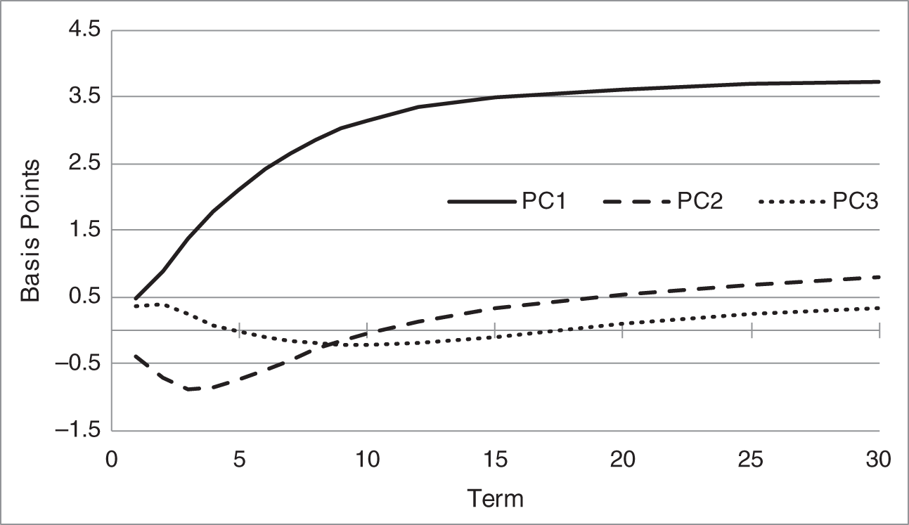
FIGURE 6.5 The First Three Principal Components of GBP LIBOR Swap Rates, Estimated from June 1, 2020, to July 16, 2021.
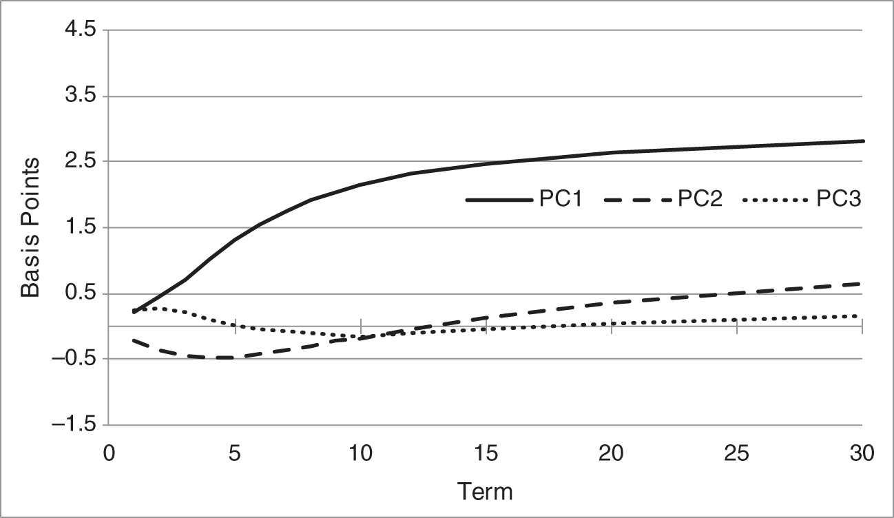
FIGURE 6.6 The First Three Principal Components of Euribor Swap Rates, Estimated from June 1, 2020, to July 16, 2021.
TABLE 6.6 USD LIBOR Par Swap Rates and DV01s, as of July 16, 2021, and PC Elements from Table 6.5. Rates Are in Percent, and PC Elements Are in Basis Points.
| Term | Rate | DV01 | Level | Slope | Short Rate |
|---|---|---|---|---|---|
| 10 | 1.303 | 0.09347 | 3.44 | 0.07 | −0.23 |
| 15 | 1.501 | 0.13387 | 3.65 | 0.71 | 0.00 |
| 20 | 1.596 | 0.17064 | 3.73 | 1.02 | 0.17 |
| 30 | 1.646 | 0.23600 | 3.77 | 1.35 | 0.36 |
This section illustrates hedging with PCA in a context described earlier, namely, hedging a relative value 10s‐20s‐30s butterfly, but this time in swaps. Specifically, a trader believes that USD 20‐year swap rates are too high relative to 10‐ and 30‐year swap rates, and plans, therefore, to receive fixed in 20s and pay in 10s and 30s.8 Par swap rates and DV01s of par swaps are given in Table 6.6. Also, corresponding to rates of the listed terms, the table gives the elements of each of the three PCs from Table 6.5. By definition, a one standard deviation shift in each PC changes these swap rates by these PC elements. The inclusion of the 15‐year swap rate is discussed later.
Assume that the trader plans to receive fixed on 100 notional amount of the 20‐year swap and on ![]() and
and ![]() notional amount of 10‐ and 30‐year swaps, respectively. Paying fixed is reflected, in this notation, with negative notional amounts. In any case, from the data in Table 6.6, the exposure of this overall relative value portfolio is hedged against a one standard deviation shift of the level and slope PCs, respectively, if the following equations obtain,
notional amount of 10‐ and 30‐year swaps, respectively. Paying fixed is reflected, in this notation, with negative notional amounts. In any case, from the data in Table 6.6, the exposure of this overall relative value portfolio is hedged against a one standard deviation shift of the level and slope PCs, respectively, if the following equations obtain,
The first two terms of Equation (6.30) give the change in the value of the hedge position under a one standard deviation shift of the first PC, that is, a shift of +3.44 basis points in the 10‐year and +3.77 basis points in the 30‐year swap rate. The third term gives the change in the value of the position being hedged under the same PC shift, which is +3.73 basis points in the 20‐year swap rate. Note that the negative signs indicate that receiving fixed (i.e., positive notional amounts) when rates increase results in position losses. The equation as a whole, therefore, sets the total position gain or loss under a one standard deviation shift of the first PC equal to zero. Equation (6.31) can be interpreted similarly, but under a one standard deviation shift of the second PC. Note, of course, that if these two equations hold for a one standard deviation shift, they hold for any size shift: to see this, simply multiply both sides of each equation by the intended number of standard deviations.
Solving Equations (6.30) and (6.31) reveals that ![]() and
and ![]() . Or, in terms of risk weights relative to the DV01 of the 20‐year swap,
. Or, in terms of risk weights relative to the DV01 of the 20‐year swap,
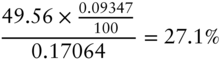
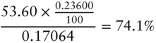
Intuitively, most of the risk of the 20‐year swap – 74% – is hedged with 30‐year swaps, because the exposures of 20‐year swaps to both the level and slope PCs more closely resemble those of 30‐year swaps than of 10‐year swaps. Note also that the sum of the risk weights is 101.2%, so that the DV01 of the hedge position is greater than the DV01 of the position being hedged. Only under the assumption of parallel shifts do the risk weights always sum to 100%. In the present case, more DV01 risk is needed in the hedge because the hedge includes a significant amount of 10‐year swaps, which are much less sensitive to the level and slope shifts than the 20‐year swaps.
In this illustration, the trader chooses to hedge with 10‐ and 30‐year swaps. But, with only two hedging securities, the risks of only two PCs can be hedged. What is the risk of the hedged position just derived to the next most important PC, that is, the short‐rate or curvature PC? Following the same logic as in Equations (6.30) and (6.31), the exposure of the hedged position to the third PC (adding a significant digit to avoid confusion) is,
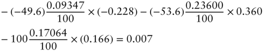
which is less than one cent per 100 face amount. The trader might very well decide, therefore, that it is not worth the transaction costs of trading an additional swap to hedge out this residual risk from the third PC. Also, because this is a relative value trade, the trader wants to pay fixed only in swaps with rates that are believed to be too low. In any case, if hedging out the residual risk is desired, a 15‐year swap can be added to the hedging portfolio; an equation for exposure to the third PC can be added to Equations (6.30) and (6.31); and, using the data from Table 6.6, the notional amounts for the 10‐, 15‐, and 30‐year swaps can be determined. This is left as an exercise for the reader.
NOTES
- 1 A linear estimator is linear in the observations of the dependent variable. The expectation of an unbiased estimator of a parameter equals the true value of that parameter. A consistent estimator of a parameter, with enough data, becomes arbitrarily close to the true value of the parameter. And an efficient estimator has the minimum possible variance among linear estimators.
- 2 A standard error is actually the sum of the squared residuals divided by the number of observations minus two, while a standard deviation divides by the number of observations minus one. Note than, in a regression with a constant, the average of the residuals is zero by construction.
- 3 While it is usual to include a constant term in the change‐on‐change regression, the constant is omitted here for expositional purposes.
- 4 See Equation (A6.15) in Appendix A6.1, which expresses the variance of the P&L as a quadratic in the DV01s of each position.
- 5 LIBOR swaps are being phased out at the time of this writing, but a sufficiently long time series of liquid SOFR swap rates is not yet available for the analysis of this section.
- 6 For many years before the financial crisis of 2007–2009, the first PC was hump‐shaped, increasing to a peak at about five years or so, and then declining gradually over longer terms. This shape was interpreted as the Federal Reserve pegging very short‐term rates but responding in the relatively near term to economic volatility. Also, because current economic volatility affects views on longer‐term rates less and less with term, volatility eventually begins to decline with term. Current Federal Reserve policy, however, as discussed in the text, seems to have changed dramatically this empirical feature of rates markets.
- 7 For a description of these floating‐rate indexes, see Chapter 12.
- 8 From the material presented in Chapter 2, the reader can think of this trade as “buying” 20‐year bonds and “selling” 10‐ and 30‐year bonds.