
CHAPTER 16
Fixed Income Options
This chapter describes some of the more common fixed income options, namely: callable bonds, which have embedded options; Euribor futures options, which are futures‐style options; bond futures options, which are equity‐style options; caps and floors; and swaptions. The reader is assumed to have some familiarity with the basics of options and options pricing. Also, with the transition to LIBOR replacements still in process at the time of this writing, caps and floors and swaptions are presented in terms of LIBOR.
While fixed income options are sometimes priced using term structure models, along the lines of Chapters 7 through 9, this chapter focuses on pricing with variations of the Black‐Scholes‐Merton (BSM) option pricing model. This simpler approach is often used by practitioners when the objective is not to determine which options among many are relatively cheap or rich, but rather to interpolate the prices of some options from the prices of similar, but more liquid options, and to calculate usefully accurate deltas or hedge ratios. An extensive appendix justifies the use of BSM in each case with mathematically simplified versions of modern asset pricing techniques.
16.1 EMBEDDED BOND CALL OPTIONS
There is not much of a market for stand‐alone options on bonds, but many corporate bonds include call provisions that give the issuer the right to call or buy back its bonds at some fixed schedule of prices. These provisions are called embedded options, because they do not trade separately or independently of the bonds. In any case, the relevant institutional background is given in Chapter 14. This section, for purposes of discussion, takes as an example the Bank of America (BoA) 2.305s of 02/22/2039, which were issued in February 2019. They are callable by BoA on February 22, 2029, at par, or 100% of face value. Table 16.1 lists this bond, along with two others that are used in this section as reference bonds. All three bonds are denominated in euros, and they were issued by banks that, as of the pricing date, are rated A2 by Moody's. Only the BoA bonds, however, are callable. The DZ Bank bonds mature on the date the BoA bonds are callable, and the Banco Santander bonds mature on the same date as the BoA bonds.
TABLE 16.1 Callable Bank of America Bond and Two Reference Noncallable Bonds. All Cash Flows Are Denominated in Euros. Prices Are as of August 23, 2021. Coupons Are in Percent.
| Issuer | Coupon | Maturity | Call Provisions | Price |
|---|---|---|---|---|
| Bank of America | 2.305 | 02/22/2039 | Callable on 02/22/29 @100 | 113.296 |
| DZ Bank | 0.75 | 02/22/2029 | Noncallable | 104.566 |
| Banco Santander | 2.28 | 02/28/2039 | Noncallable | 118.044 |
BoA will exercise its call option if rates on the call date are low relative to BoA's cost of funds. For example, if BoA can issue new 10‐year debt at 1.75% as of the call date, it will likely call the 2.305s of 02/22/2039 at a price of 100 and raise the funds to do so by selling new, 10‐year debt at 1.75%. In this way, BoA reduces its interest cost over the subsequent 10 years from 2.305% to 1.75%. On the other hand, if BoA's cost of new 10‐year debt is 2.50% on the call date, it will not exercise its option, and it will leave outstanding its 2.305s of 02/22/2039. Return then to Table 16.1. If rates are low as of the pricing date, it is more likely that the BoA bonds will be called in 2029, which is the maturity of the DZ Bank bonds. If, on the other hand, rates are high as of the pricing date, it is less likely that the BoA bonds will be called in 2029, that is, more likely that they will remain outstanding until 2039, which is the maturity of the Banco Santander bonds. Hence, the effective maturity and duration of the BoA bonds changes from that of a 7.5‐year bond, when rates are low and the call is very likely to be exercised, to that of a 17.5‐year bond, when rates are high and the call is very unlikely to be exercised.
Because the BoA embedded call is a European‐style option, it is particularly suitable for pricing by BSM.1 More specifically, consider a fictional, noncallable BoA bond with a coupon of 2.305% and a maturity of February 22, 2039. The embedded call provision is then a call option on that fictional, underlying bond struck at par, and the value of the BoA callable bond equals the value of the underlying bond minus the value of the option. Essentially, bondholders own the underlying noncallable bond and have sold a call option to the issuer to buy that bond at par.
The BSM approach to pricing the BoA embedded call option is laid out in Table 16.2. Under the assumption that the forward underlying bond price is lognormally distributed, Appendix A16.3 shows that the value of a call on a bond is,
TABLE 16.2 Pricing the Embedded Call Option of the Bank of America 2.305s of 02/22/2039, as of August 23, 2021.
| Quantity | Value |
|---|---|
| 103.732 | |
| 7.496 | |
| 100 | |
| 5.238% | |
| 0.990 | |
| 7.877 | |
| 7.797 | |
| Forward Rate: August 2021 to Feb 2029 | 0.137% |
| Forward Rate: Feb 2029 to Feb 2039 | 2.050% |
| Spread | |
| (Fictional) Noncallable Price | 122.347 |
| Callable Price | 114.551 |
where ![]() is the discount factor to the option expiration date,
is the discount factor to the option expiration date, ![]() ;
; ![]() is the forward price of the underlying bond for delivery on date
is the forward price of the underlying bond for delivery on date ![]() ;
; ![]() is the strike price; and
is the strike price; and ![]() is the volatility, which, under the lognormal assumption, is expressed as a percentage of price. The function
is the volatility, which, under the lognormal assumption, is expressed as a percentage of price. The function ![]() is as given in Appendix A16.4.
is as given in Appendix A16.4.
Two of the required inputs of (16.1) are not easily available, namely the forward price to the call date of the fictional, underlying bond, and the volatility. There are several ways to estimate these missing values, but Table 16.2 takes the following approach. First, find the two forward rates – one from the pricing date to the BoA bond's call date, and one from the call date to the BoA bond's maturity date – that recover the prices of the DZ Bank and Banco Santander reference bonds. Then, using these rates, calculate that the forward price of the underlying BoA bond is 102.29. Second, assume that the relevant volatility is 59.8 basis points, which is that of an at‐the‐money (ATM) EUR swaption with an option expiration of seven years and an underlying tenor of 10 years, which terms are close to that of the embedded call option. Then, convert this basis‐point volatility to a percentage volatility. The DV01 of the underlying forward bond, using the term structure just described, is 0.0896. Therefore, a volatility of 59.8 basis points corresponds to a price volatility of 59.8 times 0.0896, or 5.36, which, in turn, corresponds to a percentage price volatility of ![]() , or 5.24%. Not surprisingly, pricing the callable bond with this forward price and volatility does not exactly match the observed market price of 114.551 (including accrued interest). The third and final step, therefore, is to add a spread to the constructed forward rates that recovers the market price of the BoA callable bond. More precisely, for any spread, calculate the price of the underlying bond; calculate the value of the call option; and calculate the value of the callable bond as the difference between those two values. Iterate on the spread until the callable bond value equals its market price. Through this iteration, by the way, the percentage price volatility is kept constant at the 5.24% calculated previously. In any case, Table 16.2 reports the final numbers. The resulting spread is about minus 16 basis points, which increases the previously calculated underlying forward price to 103.732, and the resulting option value is 7.797. Within this framework, of course, a trader could calculate the DV01 of the callable bond, which can be used quantify, manage, or hedge its interest rate risk.
, or 5.24%. Not surprisingly, pricing the callable bond with this forward price and volatility does not exactly match the observed market price of 114.551 (including accrued interest). The third and final step, therefore, is to add a spread to the constructed forward rates that recovers the market price of the BoA callable bond. More precisely, for any spread, calculate the price of the underlying bond; calculate the value of the call option; and calculate the value of the callable bond as the difference between those two values. Iterate on the spread until the callable bond value equals its market price. Through this iteration, by the way, the percentage price volatility is kept constant at the 5.24% calculated previously. In any case, Table 16.2 reports the final numbers. The resulting spread is about minus 16 basis points, which increases the previously calculated underlying forward price to 103.732, and the resulting option value is 7.797. Within this framework, of course, a trader could calculate the DV01 of the callable bond, which can be used quantify, manage, or hedge its interest rate risk.
Figure 16.1 illustrates the interest rate behavior of callable bonds by graphing the prices of the three bonds in Table 16.7 against the yield of the Banco Santander bonds. The start of the pandemic and economic shutdowns is omitted, leaving pre‐pandemic data, from April 30, 2019, to February 28, 2020, and post‐pandemic data from May 4, 2020, to September 17, 2021. The Banco Santander and DZ Bank bonds, which are not callable, have price–yield relationships that are close to linear. These curves are actually positively convex, of course, like all fixed‐coupon bonds, but the nonlinearities are too small to be seen in the figure. Prices of the DZ Bank bond are relatively low, because of its low coupon. The price–yield curves of both the DZ Bank bond and the Banco Santander bond are downward sloping, of course, but the DZ curve is relatively flat, while the Santander curve is relatively steep, because the former matures in 7.5 years and the latter in 17.5 years. The price behavior of the callable BoA bond, however, is quite different, as it displays sharp and noticeable negative convexity. At high yield levels, where the likelihood of its being called in the future is low, its price–yield behavior resembles that of the similar‐maturity Banco Santander bond. On the other hand, at low yield levels, where the likelihood of its being called in the future is high, its price sensitivity to rates declines: investors are likely to enjoy the now relatively high‐coupon of the bond for only another 7.5 years, not for another 17.5 years. Hence, the slope of the BoA bond's price‐yield curve flattens and approaches that of the 7.5‐year DZ Bank bond. The BoA bonds seem to have experienced a particularly large price drop relative to Banco Santander bonds after the pandemic. This might be a divergence of issuer‐specific spreads, or it might be that increased rate volatility increased the value of the embedded call and reduced the price of the callable bond.
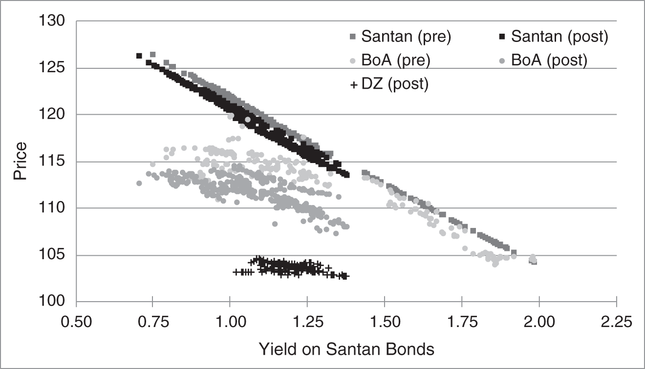
FIGURE 16.1 Prices of the Banco Santander 2.28s of 02/28/2039, the Bank of America 2.305s of 02/22/2039, and the DZ Bank 0.75s of 02/22/2029, Against the Yield of the Santander Bonds. The “Pre‐Pandemic” Period Is April 30, 2019, to February 28, 2020, and the “Post‐Pandemic Period” Is May 4, 2020, to September 17, 2021. The DZ Bank Bonds Were Issued in February 2021.
Many callable bonds have more complex call provisions that that of the BoA bonds. For example, a new 30‐year bond with a coupon of 5% might be callable in 10 years at a price of 102.50, and callable thereafter at prices that decline gradually each year until reaching 100. When this bond is issued, and the first call date is 10 years distant, most of the value of the call is at that first date and the BSM approach described in this section might be perfectly adequate. To elaborate, if the bond is unlikely to be called in 10 years at a price of 102.50, it is also unlikely to be called in 11 years at a price of, say, 102.375. Closer to the period over which the call provision is live, however, its American or Bermudan features can become more important, and the European‐style assumption of BSM becomes less suitable. In these situations, it is more appropriate to apply a term structure model along the lines of Chapters 7 through 9:
- Create an appropriate risk‐neutral tree of short‐term rates. In some cases the short‐term rate process is designed to price bonds of the issuer selling the callable bond, but in most cases the process would correspond to a swap or government bond benchmarks. A firm‐ or bond‐specific spread or option‐adjusted spread (OAS) would then be added to rates for bond valuations.
- Using the risk‐neutral tree methodology, calculate the value along the tree of an otherwise identical, noncallable bond, that is, a noncallable bond with the same scheduled coupon and principal payments as the callable bond being priced.
- Calculate the value along the tree of the call option embedded in the callable bond. Consistent with the well‐known methods for pricing American‐ or Bermudan‐style options along a tree, start from the maturity date of the option and work backwards, using the rules that i) the value of the option at any node equals the maximum of the value of immediately exercising the option and the value of holding the option for another period; and ii) the value of holding the option for another period at any node is its expected discounted value in the risk‐neutral tree.
- The value of the callable bond equals the value of the otherwise identical noncallable bond minus the value of the option.
With this valuation procedure in place, other computations are straightforward. Given a market price for the callable bond, an OAS can be computed along the lines of Chapter 7. Also, an option‐adjusted duration (OAD) or DV01 can be calculated by perturbing the short‐term rate factor and repeating steps 1 to 4 or, for a metric more similar to yield‐based sensitivities, by perturbing the initial term structure and repeating the valuation procedure.
16.2 EURIBOR FUTURES OPTIONS
Euribor futures contracts are discussed in Chapter 12. Options on Euribor futures are futures‐style options, because, like futures, all of their profits or losses are in the form of daily settlement payments. To explain the workings of this kind of option, consider a futures‐style call option with a strike of 97.0 on some underlying futures contract. If the futures price at the expiration of the option is 99.0, then the final settlement price of the call option is 99.0 minus 97.0, or 2.0. If the futures price at expiration of the option is 95.0, then the final settlement price of the call option is zero. In other words, the final settlement price of the call option is its intrinsic value, that is, the maximum of zero and the difference between the underlying price and the strike.2
Now say that a trader buys the 97 call sometime before expiration at a price of 0.20. Because this is a future‐style option, the trader does not pay that 0.20 as a premium. Instead, the trader enters into the option contract like any other futures contract: the current contract price is 0.20, and all subsequent changes in the option price trigger daily settlement payments. If, at expiration, the underlying futures price is 99, the final settlement of the 97 call is 2.0, and the total of the trader's daily settlement payments will have been 2.0 minus 0.20, or 1.80. Hence, the total profit of the trader is the same 1.80 as that of a traditional call option – the final underlying price of 99, minus the strike of 97, minus the premium of 0.20. But in the case of the futures‐style option, that 1.80 is realized as a sequence of daily settlement payments. Similarly, if, at expiration, the underlying futures price is 95.0, the final settlement price of the 97 call is zero, and the total of the trader's daily settlement payments will have been negative 0.20. Again, the total payoff is the same as that of a traditional call option that finishes out‐of‐the‐money, that is, the loss of the premium, but this loss is realized in the form of daily settlement payments.
As explained in Chapter 12, the price of a Euribor futures contract is set to 100 minus its percentage rate. In the example of the previous paragraph, the strike price of 97 corresponds to a rate of (100 − 97)/100, or 3%, and the final underlying futures settlement price of 99 corresponds to a rate of 1%. Furthermore, as also explained in Chapter 12, Euribor futures contracts are scaled so that a decline of one basis point in rate is worth €25. Hence, the difference between the strike and final settlement rates, which is 3% minus 1% or 200 basis points, is worth 200 times €25, or €5,000. More generally, if the call option strike in terms of rate is ![]() , and the final settlement rate of the underlying futures contract is
, and the final settlement rate of the underlying futures contract is ![]() , then the final settlement price of the call option is,
, then the final settlement price of the call option is,
where ![]() is shorthand for the maximum of
is shorthand for the maximum of ![]() and 0, and the factor of 10,000 simply converts the rate gain, if any, to basis points, so as to be multiplied by €25. Analogously, the payoff of a put option on a rates futures contract is,
and 0, and the factor of 10,000 simply converts the rate gain, if any, to basis points, so as to be multiplied by €25. Analogously, the payoff of a put option on a rates futures contract is,
Equations (16.2) and (16.3) show that a call option on the futures price can be expressed as a put option on its rate, and a put option on the price can be expressed as a call option on its rate. With this insight and the assumption that futures rates are normally distributed, Appendix A16.3 shows that the prices of call and put options on Euribor futures are given by the following expressions, respectively,
TABLE 16.3 A 100.25 Call on September 2022 Three‐Month Euribor Futures, as of February 28, 2022. The Futures Price Is 100.235. The Contract and Option Mature on September 19, 2022.
| Quantity | Value |
|---|---|
| −0.2350% | |
| −0.25% | |
| 0.6842% | |
| 0.1961% | |
| €490.34 |
where ![]() is the current futures rate;
is the current futures rate; ![]() is the time to option expiration in years;
is the time to option expiration in years; ![]() is the strike, in terms of rate; and
is the strike, in terms of rate; and ![]() is the basis‐point volatility of the futures rates. The functions
is the basis‐point volatility of the futures rates. The functions ![]() and
and ![]() are as given in Appendix A16.4. Note that these formulae are not preceded by a discount factor, because these options are themselves futures: their prices equal their expected value under the risk‐neutral measure, or equivalently, there is no initial premium on which a return need be earned. Also, the BSM model is readily applied here, because American futures‐style options are not optimally exercised early: with daily settlement of the option value, there is no intrinsic value to be realized by exercise and, therefore, no reason to sacrifice the remaining time value of the option.
are as given in Appendix A16.4. Note that these formulae are not preceded by a discount factor, because these options are themselves futures: their prices equal their expected value under the risk‐neutral measure, or equivalently, there is no initial premium on which a return need be earned. Also, the BSM model is readily applied here, because American futures‐style options are not optimally exercised early: with daily settlement of the option value, there is no intrinsic value to be realized by exercise and, therefore, no reason to sacrifice the remaining time value of the option.
Table 16.3 applies Equation (16.4) to a call on the September 2022 Euribor futures contract with a strike of 100.125. As of the pricing date, the futures price is 100.235, which corresponds to a rate of ![]() 0.2350%. The futures contract and the option both mature on September 19, 2022, which is 203 days from the pricing date.
0.2350%. The futures contract and the option both mature on September 19, 2022, which is 203 days from the pricing date.
16.3 BOND FUTURES OPTIONS
Bond futures in the United States are discussed in Chapter 11. Options on these futures contracts are traditional or equity‐style options, which means that, like options on stocks, purchasers of options pay a premium at the time of purchase and, if exercised, realize their intrinsic values.
Options on bond futures can be valued with term structure models. In a one‐factor model, for example, after creating a risk‐neutral tree for the futures price, the value of a futures option can be computed by starting from the maturity date of the option and working backwards, using the rule that the value of the option at each node is the maximum of the value of holding the option and of exercising it immediately. Of course, because the delivery options embedded in bond futures may not be modeled adequately by a one‐factor model, multi‐factor approaches might be preferred.
While simple conceptually, it is apparent from Chapter 11 that building a futures model takes a good deal of effort. Therefore, practitioners who do not otherwise need such a model tend to use a BSM approach for bond futures options. The required assumptions are that: the option is European; the discount factor to option expiration is uncorrelated with the underlying futures price; and the futures price is lognormal with constant volatility. The assumption that the option is European, that is, that early exercise is not optimal, is reasonable in practice. Early exercise of an equity‐style futures option may be optimal if interest earned on the realized intrinsic value exceeds the time value of the option, but this is rarely the case. For some intuition on this point, note that early exercise of a put on a stock may be optimal, because of the potential of earning interest on the entire strike price, not just on its intrinsic value. The assumption that the discount factor is uncorrelated with the bond futures price is not bad in practice. Bond futures options typically mature in a few months or less, while the bond underlying the futures contract typically matures in many years. Hence, the correlation is typically weak between the discount factor, which depends on very short‐term rates, and the bond futures price, which depends on longer‐term rates. The assumption of constant price volatility, however, essentially assumes away the delivery options of bond futures: as rates change and the cheapest‐to‐deliver bond changes, the DV01 and, therefore, the price volatility of the futures changes as well. (See Chapter 11.) While perhaps acceptable when interest rates are low relative to the contract's notional coupon, ignoring the delivery option seems to undercut one of the main motivations for using BSM in the first place, namely, to obtain accurate deltas. Nevertheless, BSM is used in practice in this context.
Under the assumptions listed in the previous paragraph, Appendix A16.3 shows that calls and puts on US Treasury note and bond futures contracts are given by, respectively,
where ![]() is the face amount of bonds per contract;
is the face amount of bonds per contract; ![]() is the futures price;
is the futures price; ![]() is the time to option expiration;
is the time to option expiration; ![]() is the strike price;
is the strike price; ![]() is the lognormal or percentage price volatility; and
is the lognormal or percentage price volatility; and ![]() is the discount factor to option expiration. Table 16.4 applies Equation (16.6) to a call option on the June 10‐year US Treasury note futures contract as of the end of February 2022, where both the futures and option contracts expire on June 21, 2022. Note that there are 113 days from February 28, 2022, to June 21, 2022.
is the discount factor to option expiration. Table 16.4 applies Equation (16.6) to a call option on the June 10‐year US Treasury note futures contract as of the end of February 2022, where both the futures and option contracts expire on June 21, 2022. Note that there are 113 days from February 28, 2022, to June 21, 2022.
TABLE 16.4 A Call Option on the June 10‐Year Treasury Note Futures Contract, as of February 28, 2022. The Futures Contract and Option Mature on June 21, 2022.
| Quantity | Value |
|---|---|
| 126.3438 | |
| 126.5 | |
| 5.655% | |
| 0.9979% | |
| 1.50996 | |
| $1,509.96 |
16.4 CAPS AND FLOORS
The easiest way to describe caps is to start with caplets, even though caps are the more traded derivative. At the end of a given accrual period, a caplet pays the greater of zero and of LIBOR minus a strike, where LIBOR is set at the beginning of the accrual period. Consider, for example, a caplet with a three‐month LIBOR reset date of February 14, 2022, a payment date of May 14, 2022, and a strike of .181%. Note that there are 89 days over this accrual period. If LIBOR on February 14, 2022, turns out to be ![]() , then a unit notional of the caplet will pay, on May 14, 2022,
, then a unit notional of the caplet will pay, on May 14, 2022,
where, as mentioned already, ![]() is another way of writing max
is another way of writing max ![]() . Note that the payoff of a caplet looks like that of an option, but the maximum is a feature of the contract rather than a result of optimal exercise behavior.
. Note that the payoff of a caplet looks like that of an option, but the maximum is a feature of the contract rather than a result of optimal exercise behavior.
Caplets are typically valued by practitioners under the assumption that forward LIBOR rates are normally distributed. Under this assumption, Appendix A16.3 shows that the value of a caplet with a reset at time ![]() and payment at time
and payment at time ![]() +
+ ![]() is given by,
is given by,
where ![]() is the term of the reference rate;
is the term of the reference rate; ![]() is the discount factor to the payment date;
is the discount factor to the payment date; ![]() is today's forward rate from
is today's forward rate from ![]() to
to ![]() ;
; ![]() is the strike;
is the strike; ![]() the basis‐point volatility of the forward rate; and
the basis‐point volatility of the forward rate; and ![]() the BSM‐style formula defined in Appendix A16.4. Table 16.5 applies Equation (16.9) to 100 notional of the caplet introduced previously, as of May 14, 2021. Note that there are 276 days from the pricing date, May 14, 2021, to the reset date, February 14, 2022.3 The appropriate discount factor to the payment date, derived from the swap curve, is .998191. Finally, a volatility of 12.09 basis points, which comes from the discussion, is used to derive the price of .0129 cents per 100 notional amount.
the BSM‐style formula defined in Appendix A16.4. Table 16.5 applies Equation (16.9) to 100 notional of the caplet introduced previously, as of May 14, 2021. Note that there are 276 days from the pricing date, May 14, 2021, to the reset date, February 14, 2022.3 The appropriate discount factor to the payment date, derived from the swap curve, is .998191. Finally, a volatility of 12.09 basis points, which comes from the discussion, is used to derive the price of .0129 cents per 100 notional amount.
A cap is a portfolio of caplets, with the value of the cap being the sum of the value of its component caplets. The implied volatility of a cap is the volatility that, when used to value every component caplet, results in the market price of the cap. This leads to some complexities, as will be discussed presently, because the term structure of caplet volatility is not flat. In other words, every caplet is properly valued at its own volatility even though, when quoting the price of a cap, all of its component caplets are valued at a single, cap volatility.
TABLE 16.5 Pricing a Caplet with a LIBOR Reset on February 14, 2022, and a Payment Date on May 14, 2022, as of May 14, 2021.
| Quantity | Value |
|---|---|
| .200% | |
| .181% | |
| .1209% | |
| .998191 | |
| .00052 | |
| .0129 |
Table 16.6 illustrates the structure of a cap and cap pricing with a one‐year US dollar ATM cap as of May 14, 2021. This cap is ATM because its strike of 0.181% equals the rate of the corresponding swap, which, in this case, is the one‐year swap. The cap strike of 0.181% means that every component caplet has a strike of 0.181%. The cap volatility of 12.09 basis points means that the price of the cap is the sum of the component caplet values when each caplet is valued at a volatility of 12.09 basis points. The forward rates are derived from the swap curve, and the caplet premiums are calculated from the normal BSM formula, with: each respective forward rate; a strike of 0.181%; a volatility of 12.09 basis points; and appropriate date parameters and discount factors along the lines of Table 16.5. In fact, the caplet in Table 16.6 that pays on May 14, 2022, is the same caplet that is valued in Table 16.5.
Note that what might have been the first caplet in Table 16.6, with a LIBOR reset at the start of the cap initiation and a payment on August 14, 2021, is omitted from the table. The payment from such a caplet is known as of the start of the cap and, as such, has no option‐like premium: it is simply worth its present value. In fact, in this example, where the initial LIBOR setting is below the strike, at .155%, the payment from this caplet is zero. In any case, along these lines, the first caplet payment is usually omitted from a cap.
The one‐year cap in the example is a spot starting cap; that is, putting aside the skipping of the first payment, the schedule of payments starts immediately. There is also an active market, however, in forward starting caps. In a 5 ![]() 5 cap, the first reset is in five years, the first payment in five years plus the length of the accrual period (e.g., five years and three months), and the last payment in 10 years.
5 cap, the first reset is in five years, the first payment in five years plus the length of the accrual period (e.g., five years and three months), and the last payment in 10 years.
As mentioned before, if caplets traded individually, they would be priced at individual volatilities, not at a single, cap volatility. In other words, there is a term structure of caplet volatilities. This term structure is interesting for use as another perspective on the market price of volatility and for comparison with – and perhaps trading opportunities against – other volatility instruments. In theory, the term structure of caplet volatility could be recovered from caps of sequential terms. The problem is complicated, however, by the fact that the most traded and useful volatilities are ATM volatilities, which, in the case of caplets, correspond to caplets with strikes equal to their underlying forward rates. But the strikes of caplets that are part of caps all have a single strike that cannot, in general, equal the underlying forward rate for every component cap. Furthermore, as discussed presently, the volatilities of options that are and are not ATM can be significantly different from each other. Hence, the extraction of caplet volatilities from caps is often combined with some adjustment for the caplet strikes not being ATM.
TABLE 16.6 The Structure and Pricing of a One‐Year Cap as of May 14, 2021. Rates Are in Percent.
| Cap Strike | .181% | ||
|---|---|---|---|
| Cap Volatility | .1209% | ||
| Dates | |||
| Reset | Payment | Forward Rate | Caplet Premium |
| 05/14/2021 | 08/14/2021 | .155 | |
| 08/14/2021 | 11/14/2021 | .160 | .0039 |
| 11/14/2021 | 02/14/2022 | .200 | .0114 |
| 02/14/2022 | 05/14/2022 | .200 | .0129 |
| Sum | .0281 | ||
Floorlets and floors are analogous to caplets and caps. The payment of a floorlet at time ![]() , determined by the LIBOR rate set at time
, determined by the LIBOR rate set at time ![]() , is,
, is,
Assuming normal forward rates, the value of a floorlet is given by,
where the function ![]() is given in Appendix A16.4. The value of a floor is the sum of the values of its component floorlets.
is given in Appendix A16.4. The value of a floor is the sum of the values of its component floorlets.
Applying put‐call parity, the prices of an ATM caplet and an ATM floorlet with the same expiration are equal, as are the prices of matched‐date ATM caps and floors. Say, for example, that the five‐year swap rate, five years forward, is 5%. Then paying fixed on this forward starting swap and buying a 5 ![]() 5 floor with a strike of 5% has exactly the same cash flows as a 5
5 floor with a strike of 5% has exactly the same cash flows as a 5 ![]() 5 cap with a strike of 5%. But, by definition, the value of the forward swap is zero. Hence, the values of the cap and the floor must be the same.
5 cap with a strike of 5%. But, by definition, the value of the forward swap is zero. Hence, the values of the cap and the floor must be the same.
16.5 SWAPTIONS
A swaption is an over‐the‐counter (OTC) contract that gives the buyer the right, at expiration, to enter into a fixed‐for‐floating interest rate swap of a prespecified maturity and strike rate. For example, a “2‐year‐5‐year” or “2y5y” swaption is a two‐year option to enter into a five‐year swap at some prespecified strike. A receiver swaption gives the buyer the right to receive fixed and pay floating, while a payer swaption gives the buyer the right to pay fixed and receive floating.
For presenting the pricing of swaptions, consider a $100 million 2.36% 5y5y receiver swaption traded on May 14, 2021. This option gives the buyer the right, in five years, on May 14, 2026, to receive 2.36% and pay LIBOR on $100 million for five years, that is, until May 14, 2031. To write down the value of this swaption at expiration, let ![]() denote the five‐year par swap rate, five years from today (which matures in 10 years), and let
denote the five‐year par swap rate, five years from today (which matures in 10 years), and let ![]() denote the value five years from today of an annuity of $1 per year, paid on each of the fixed‐rate payment dates of a five‐year swap starting in five years (and ending in 10 years). Then, in five years, at the expiration of the swaption, the value of receiving 2.36% for five years is,
denote the value five years from today of an annuity of $1 per year, paid on each of the fixed‐rate payment dates of a five‐year swap starting in five years (and ending in 10 years). Then, in five years, at the expiration of the swaption, the value of receiving 2.36% for five years is,
Inspection of the payoff (16.12) reveals that a 5y5y receiver swaption is a put on the five‐year par swap rate, five year forward. More generally, a ![]() ‐year‐
‐year‐![]() ‐year receiver swaption is a
‐year receiver swaption is a ![]() ‐year put option on the
‐year put option on the ![]() ‐year par swap rate,
‐year par swap rate, ![]() ‐years forward. Similarly, a
‐years forward. Similarly, a ![]() ‐year‐
‐year‐![]() ‐year payer swaption is a
‐year payer swaption is a ![]() ‐year call option on the
‐year call option on the ![]() ‐year par swap rate,
‐year par swap rate, ![]() ‐years forward.
‐years forward.
Table 16.7 applies BSM to the example of this section. As just discussed, the rate underlying the 2.36% 5y5y receiver option traded on May 14, 2021, is the forward par rate on a swap from May 14, 2026, to May 14, 2031. Hence ![]() of BSM is 2.36%, and the swaption of the example, with its strike at 2.36%, is ATM.4 For the 2.36% 5y5y, the other parameters are clearly
of BSM is 2.36%, and the swaption of the example, with its strike at 2.36%, is ATM.4 For the 2.36% 5y5y, the other parameters are clearly ![]() ,
, ![]() , and
, and ![]() . The value of the annuity on the swap from May 14, 2026, to May 14, 2031, as of May 14, 2021, is 4.287. Finally, the market price of this receiver option on the pricing date is 3.03 per 100 notional amount or $3.03 million on $100 million. Appendix A16.3 shows that, when the underlying forward swap rate is normally distributed, the value of a receiver swaption per unit notional is,
. The value of the annuity on the swap from May 14, 2026, to May 14, 2031, as of May 14, 2021, is 4.287. Finally, the market price of this receiver option on the pricing date is 3.03 per 100 notional amount or $3.03 million on $100 million. Appendix A16.3 shows that, when the underlying forward swap rate is normally distributed, the value of a receiver swaption per unit notional is,
where ![]() is once again from Appendix A16.4. Setting the market price of $3.03 million equal to $100 million times (16.13), Table 16.7 shows that the implied volatility of this swaption is 0.793%.
is once again from Appendix A16.4. Setting the market price of $3.03 million equal to $100 million times (16.13), Table 16.7 shows that the implied volatility of this swaption is 0.793%.
The analogous formula for a payer swaption per unit notional is,
The prices of ATM swaptions, which are by far the most commonly traded swaptions, are quoted in a matrix of either premia or implied normal volatilities. Table 16.8 is an example of the latter for US dollar swaptions as of May 14, 2021. For example, the ATM 2y10y options is priced with an implied volatility of 77.7 basis points.5 The price of the 5y5y option introduced previously is quoted at a volatility of 79.3 basis points.
TABLE 16.7 A 5y5y Receiver Swaption per 100 Notional Amount of Swaps, as of May 14, 2021.
| Quantity | Value |
|---|---|
| 2.36% | |
| 5 | |
| 5 | |
| 2.36% | |
| 0.793% | |
| 4.287 | |
| 0.007074 | |
| 3.03 mm |
TABLE 16.8 USD ATM Swaption Normal Volatilities in Basis Points, as of May 14, 2021.
| Swap Tenor | |||||||||||
|---|---|---|---|---|---|---|---|---|---|---|---|
| Option Exp. | 1y | 2y | 3y | 4y | 5y | 7y | 10y | 12y | 15y | 20y | 30y |
| 1m | 12.1 | 18.6 | 34.1 | 45.9 | 57.1 | 64.7 | 70.7 | 71.0 | 71.1 | 71.3 | 71.5 |
| 3m | 14.1 | 23.3 | 39.8 | 51.7 | 62.5 | 69.2 | 74.4 | 74.5 | 74.4 | 74.3 | 74.3 |
| 6m | 16.7 | 29.4 | 45.5 | 56.0 | 66.4 | 72.0 | 76.3 | 76.2 | 75.8 | 75.6 | 75.3 |
| 1y | 29.3 | 44.1 | 57.0 | 64.1 | 70.3 | 73.9 | 76.8 | 76.5 | 75.8 | 75.0 | 74.2 |
| 2y | 59.2 | 68.9 | 73.3 | 76.0 | 77.2 | 77.5 | 77.7 | 77.0 | 75.7 | 74.1 | 72.9 |
| 3y | 76.7 | 79.6 | 79.5 | 79.4 | 79.3 | 78.6 | 77.6 | 76.7 | 75.1 | 72.8 | 71.2 |
| 4y | 81.4 | 81.2 | 80.7 | 80.2 | 79.8 | 78.4 | 76.6 | 75.5 | 73.7 | 71.3 | 69.4 |
| 5y | 82.3 | 81.2 | 80.5 | 79.9 | 79.3 | 77.7 | 75.4 | 74.1 | 72.2 | 69.9 | 67.5 |
| 10y | 73.5 | 72.3 | 71.8 | 71.2 | 70.8 | 69.2 | 66.8 | 65.6 | 63.8 | 61.6 | 59.4 |
Swaption skew, discussed in the next section, refers to the fact that implied volatilities for ATM swaptions in Table 16.8 are valid only for ATM swaptions. The broader swaptions market, therefore, actually trades a volatility cube, where the third dimension represents strike, usually in 50 basis‐point increments away from the forward swap rate corresponding to each entry of the swaption matrix. For a 5y5y as of May 14, 2021, with the underlying par forward swap at 2.36%, a volatility cube would show volatilities for the 5y5y at higher strikes of 2.86%, 3.36%, and so forth, and for lower strikes of 1.86%, 1.36%, etc.
The skew applies not only for trading swaptions that are not ATM but also for valuing or marking existing swaptions that were initiated as ATM options. Consider the 2.36% 5y5y receiver swaption traded on May 14, 2021. The underlying swap of this swaption, from initiation to expiration, is a 2.36% swap from May 14, 2025, to May 14, 2031. As of May 14, 2021, this swap is a par swap, but over time this will no longer be the case. Say, for example, that one month later, on June 14, 2021, the rate of the forward par swap corresponding to those dates is 2.50%. In that case, the 2.36% receiver swaption can be characterized as a 4‐year‐11‐month‐5‐year that is 14 basis points out‐of‐the‐money. Valuing the option, therefore, requires an interpolation between the ATM and the 50 basis‐point, out‐of‐the‐money volatilities, as well as an interpolation between the 4y5y and 5y5y option expirations. In practice, these interpolations are carried out by means of a stochastic volatility model, discussed later in this chapter.
This section describes swaptions as if they are physically settled, meaning that, at expiration, the counterparties enter into a swap at the appropriate rate and maturity. In fact, however, swaptions in the United States are almost always cash settled and, in Europe, can be physically or cash settled. In the United States, the cash settlement is found by multiplying the appropriate annuity factor, evaluated along the swap curve, by the difference between the par rate and the strike, in the case of payers, or the difference between the strike and the par rate, in the case of receivers. In Europe, the annuity factor is computed at a flat rate equal to the appropriate par swap rate, which can lead to very minor valuation differences between the two forms of settlement. As a final note, for some swaptions in Europe, the premium is paid at the expiration date rather than the trade date, which changes valuations accordingly.
16.6 SWAPTION SKEW
The BSM normal model, as applied in the previous section, has a single and constant volatility parameter. Taking the model literally, this would imply that all swaptions can be priced with a single basis‐point volatility. Figure 16.2 illustrates, however, that this is not the case: even across swaptions with the same expiration and underlying tenor, like either the 2y2y and 5y10y swaptions in the figure, implied volatilities vary significantly with strike. As of the pricing date, the two‐year swap rate, two years forward is 1.11% (not shown in the figure), which is the ATM strike for 2y2y swaptions. The darker gray curve shows, therefore, that 2y2y implied volatilities increase mostly linearly from 56 basis points at a strike of 0.11%, which is 100 basis points below the ATM strike, to 125 basis points at a strike of 4.11%, which is 300 basis points above the ATM strike. At the same time, the 10‐year swap rate, five years forward is 2.43%. The lighter gray curve of the figure shows, therefore, that implied volatilities of 5y10y swaptions are roughly 75 basis points for strikes below that ATM strike, and then increase along the curve shown to 95 basis points at a strike 300 basis points over the ATM strike. The phenomenon that basis‐point volatility is not constant across strikes is known as the volatility skew. The phenomenon that basis‐point volatility is higher for both in‐ and out‐of‐the‐money options than for at‐the‐money options, as seen here for 5y10y swaptions, is known as the smile, or, to the extent this effect is not symmetric, the smirk.
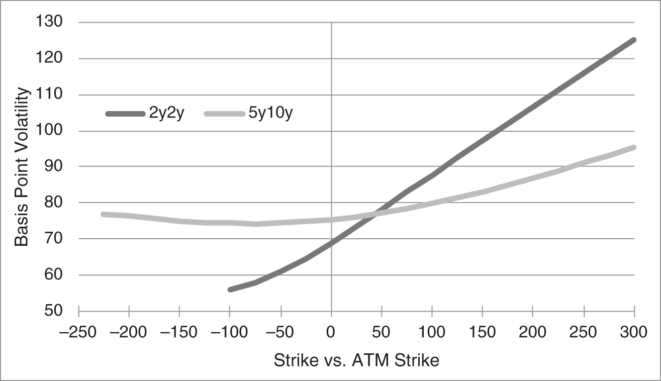
FIGURE 16.2 Implied Basis‐Point Volatilities of 2y2y and 5y10y US Dollar Swaptions Across Strikes, as of May 14, 2021.
The existence of a skew does not prevent traders from quoting swaption prices in terms of normal BSM volatility or vice versa, so long as the volatilities vary with strike. But practitioners rely on BSM not just to quote a price or volatility, but also to compute delta, that is, to compute how the value of a swaption changes as its underlying forward rate changes. And the usefulness of BSM for this purpose is cast into doubt by Figure 16.2. Without getting into great detail here, the implied volatility of an option at a given strike can be thought of as the expected gamma‐weighted average of instantaneous volatilities over possible paths of the underlying forward rate as it changes from its current level to the strike. From this perspective, the implied volatility curves in Figure 16.2 mean that instantaneous volatilities vary in a complex way with the level the forward rate. In that case, however, the value of an option changes with the level of rates in two ways: a direct effect, that is, the change in the underlying forward; and an indirect effect, that is, the change in volatility as a result of the change in the level of rates. But the BSM delta, which is traditionally computed as the change in option value for a change in the underlying at a given volatility, captures only the direct effect.
The search for a model that can capture the underlying dynamics of volatility as a function of forward rates has taken two very broad paths. The first is to change the distribution of the forward rate away from normal. For example, a constant‐volatility lognormal model of rates assumes that volatility is proportional to rates, which might be useful in explaining some manifestations of the skew, like parts of the 2y2y curve in Figure 16.2. In any case, along these lines, the shifted lognormal model allows for the distribution of the underlying forward rate to be between normal and lognormal. The defining dynamics of the forward rate, ![]() , in this model are,
, in this model are,
with ![]() . When
. When ![]() ,
, ![]() , the basis‐point volatility in Equation (16.15) is just
, the basis‐point volatility in Equation (16.15) is just ![]() , that is, a constant proportion of the forward rate. Therefore, the distribution of the rate is lognormal. At the other extreme, as
, that is, a constant proportion of the forward rate. Therefore, the distribution of the rate is lognormal. At the other extreme, as ![]() approaches infinity,
approaches infinity, ![]() in (16.17) approaches the constant
in (16.17) approaches the constant ![]() , which means that the volatility in (16.15) approaches a constant and, therefore, that the distribution approaches normality.
, which means that the volatility in (16.15) approaches a constant and, therefore, that the distribution approaches normality.
The second approach to finding a model that captures the relationship between rates and volatility is to allow volatility itself to be a random variable. This approach leads to stochastic volatility models, in which class the SABR model had proven particularly popular. As originally formulated, however, the model could not handle the negative rates that recently characterized markets in Europe. An adjusted model then emerged, known as the shifted‐SABR model, which assumes the following dynamics,
with ![]() ,
, ![]() ,
, ![]() , and
, and ![]() . There are several features to note about this formulation. First, the only difference between this model and the original SABR model is the shift parameter,
. There are several features to note about this formulation. First, the only difference between this model and the original SABR model is the shift parameter, ![]() . With this shift, the forward rate
. With this shift, the forward rate ![]() can be as negative as
can be as negative as ![]() with the basis‐point volatility of the model –
with the basis‐point volatility of the model – ![]() – still positive. Second, the SABR model approaches the normal model as both
– still positive. Second, the SABR model approaches the normal model as both ![]() and
and ![]() approach 0, and it approaches the lognormal model as
approach 0, and it approaches the lognormal model as ![]() approaches 0 and as
approaches 0 and as ![]() approaches 1. Third, the initial volatility,
approaches 1. Third, the initial volatility, ![]() , is most naturally used to match ATM swaption volatility. Fourth,
, is most naturally used to match ATM swaption volatility. Fourth, ![]() is typically less than one, because basis‐point volatilities, as illustrated in Figures 16.2, do not increase as quickly for high strikes as in a lognormal model. Fifth, the parameters
is typically less than one, because basis‐point volatilities, as illustrated in Figures 16.2, do not increase as quickly for high strikes as in a lognormal model. Fifth, the parameters ![]() and
and ![]() control the skew through controlling the relationship between the level of rates and volatility. From Equation (16.18), a higher
control the skew through controlling the relationship between the level of rates and volatility. From Equation (16.18), a higher ![]() increases the responsiveness of volatility to the level of the forward rate. And from Equation (16.22), a higher
increases the responsiveness of volatility to the level of the forward rate. And from Equation (16.22), a higher ![]() increases the correlation between changes in rates and changes in volatility. Sixth, the parameter
increases the correlation between changes in rates and changes in volatility. Sixth, the parameter ![]() controls the smile, or fat tails of the rates distribution, as a higher
controls the smile, or fat tails of the rates distribution, as a higher ![]() increases volatility when volatility is high, that is,
increases volatility when volatility is high, that is, ![]() increases volatility when rates are either higher or lower. Seventh, in practice, because the flexibility of the model enables many different sets of parameters to fit the observed skew, the parameters can also be constrained to fit empirical regularities. One popular choice, for example, is to constrain the parameters to match the empirical backbone, that is, the empirical relationship between ATM basis‐point volatilities and forward rates. Eighth, note that, in practice, a different set of parameters are typically chosen for every swaption expiration and underlying tenor. In other words, no BSM‐style model can describe the entire volatility cube.
increases volatility when rates are either higher or lower. Seventh, in practice, because the flexibility of the model enables many different sets of parameters to fit the observed skew, the parameters can also be constrained to fit empirical regularities. One popular choice, for example, is to constrain the parameters to match the empirical backbone, that is, the empirical relationship between ATM basis‐point volatilities and forward rates. Eighth, note that, in practice, a different set of parameters are typically chosen for every swaption expiration and underlying tenor. In other words, no BSM‐style model can describe the entire volatility cube.
NOTES
- 1 A European option is exercisable at expiration. An American option is exercisable at any time between a first exercise date and expiration. And a Bermudan option is exercisable on a discrete set of dates.
- 2 The final option settlement price is actually determined through the following mechanics. Exercising a call option results in having to pay the final settlement price of the option in exchange for a position in the underlying futures contract – priced at 99 in the example – at an assigned price equal to the strike of 97. That futures position and assignment results in an immediate settlement payment of 2.0. By arbitrage, then, the final settlement price of the option must be 2.0. Through these mechanics, the option is physically settled with a position in the underlying futures contract that can be kept or sold.
- 3 For simplicity, this presentation does not distinguish between business and non‐business days.
- 4 A higher strike would make the receiver swaption in‐the‐money, while a lower strike would make it out‐of‐money
- 5 ATM calls and puts have the same BSM values. This is easy to verify from Equations (A16.60) through (A16.66).