
CHAPTER 2
Swap, Spot, and Forward Rates
Chapter 1 showed that discount factors fully describe the time value of money as embedded in market prices. Investors and traders, however, often find it more intuitive to quote the time value of money in terms of interest rates and, in particular, in terms of either swap rates or par rates, spot rates, and forward rates.
This chapter begins by explaining that interest rates are always quoted as annual rates, that interest is conceptualized as being paid over a number of periods of fixed length (e.g., 90 days, three semiannual periods), and that interest rate quotations indicate the payment of either simple or compound interest. The chapter then introduces interest rate swaps (IRS) as context for the material. Swaps and bonds together comprise a significant portion of fixed income markets, and swaps, because they are relatively liquid, have become benchmarks against which to evaluate other fixed income instruments.
At the time of this writing, interest rate swap markets are in transition away from LIBOR (London Interbank Offered Rate), which has dominated floating‐rate indexes for decades. Chapter 12 discusses this transition, but this chapter briefly introduces the leading candidates for replacing LIBOR (e.g., Secured Overnight Financing Rate (SOFR) in the United States) and their associated swaps. Chapter 13 discusses why and how market participants use interest rate swaps.
2.1 INTEREST RATE QUOTATIONS
An investment with fixed cash flows is completely described by its price and cash flows. It seems enough to know, for example, that a bond paying 102 in six months costs 101.4925 today, or that a $100,000,000 1.5‐year loan made six months from today will return $103,030,100 in two years. Nevertheless, investors and traders often prefer to quote and think about valuations in terms of interest rates. As shown herein, the bond and loan just described earn semiannually compounded rates of 1% and 2% per year, respectively. Rates are more intuitive than prices and cash flows because rates automatically normalize for the amount invested and for the investment horizon. The bond costs 101.4925 and matures in six months, while the loan invests $100,000,000 in six months for 1.5 years, but their respective interest rates can be sensibly and intuitively compared.
Interest rates are always quoted as annual rates over a term or tenor, which is described as a number of periods of fixed length. A money market instrument, for example, might offer 1% per year for 90 days on an investment of $100,000. If this 1% is quoted as a simple rate of interest, under the actual/360 convention described in Section 1.7, then the interest payment at the end of the 90 days is,
If the 1% interest rate on the money market instrument is quoted not as a simple rate, but as a daily compounded rate, then interest is computed differently: the investment earns simple interest daily, but interest is earned on accumulated balances, which include interest already earned. After the first day, then, the balance includes one day of simple interest,

Over the second day, the entire balance at the end of the first day, given in Equation (2.2), earns another day of simple interest. This implies that interest is compounded, that is, the $2.78 of interest earned over the first day itself earns interest on the second day. As a result, the total balance at the end of the second day is,

where the first equality comes from substituting the left‐hand side of (2.2) for the $100,002.78 in (2.3).
Continuing in this fashion, the total balance at the end of the 90 days, which is the amount paid by the money market instrument at maturity, is,

Comparing the interest component of Equation (2.4), that is, $250.31, with that of (2.1), that is, $250.00, shows the effect of compound interest in this example. A daily compounded rate of 1% on $100,000 earns 31 cents more than a simple interest rate of 1%. When rates are higher, and when the term of the investment is longer, the difference can be much larger.
Return now to the bond and loan examples given at the start of this section. In these cases, interest is likely to be semiannually compounded, where, by convention, a semiannual period is exactly one half of a year. Therefore, the six‐month bond, which costs 101.4925 today and pays 102 after six months, earns 1% in the sense that,

The loan invests $100 million six months from today and, three semiannual periods (i.e., 1.5 years) later, returns $103,030,000. This investment earns a semiannually compounded rate of 2% in the sense that,
This section illustrates concepts with daily and semiannual periods. Daily periods are common in money markets and in the swap market discussed in the next section. Semiannual periods are common in many government and corporate bond markets, like the US government bond market, discussed in Chapter 1. Different periods are used in other contexts, however. Mortgage markets use monthly periods, for example, because mortgage payments are typically paid monthly.
More generally, then, let ![]() be the number of periods per year; let
be the number of periods per year; let ![]() be the number of periods; and let
be the number of periods; and let ![]() be the interest rate to be compounded
be the interest rate to be compounded ![]() times per year. Then, investing
times per year. Then, investing ![]() at the rate
at the rate ![]() grows, after
grows, after ![]() periods, to a total balance of,
periods, to a total balance of,
Markets should ensure that the final proceeds from identical investments of the same term are the same, regardless of the compounding convention. If, for example, the market offers 102 on a 1‐year investment of 100, that investment might be quoted as earning 2% annually; 1.9901% semiannually compounded; or 1.9819% compounded monthly, because,

Note that the greater the frequency of compounding, the lower the quoted interest rate. These rates are set such that more frequent compounding, that is, paying more interest on interest, exactly offsets the lower rate earned on the initial investment.
This section concludes by noting that some contexts use continuous compounding, in which interest is conceptualized as being paid every instant. This quoting convention can appear in money markets; is frequently used at financial firms, because rates and discount factors have to be calculated at irregular intervals; and is used almost exclusively by researchers for mathematical convenience. Continuous compounding is presented in Appendix A2.1.
2.2 INTEREST RATE SWAPS
In an interest rate swap, two parties agree to exchange a series of interest payments. Consider first the solid arrows in Figure 2.1, which are the only contractual cash flows of the depicted swap. Counterparty A agrees to pay Counterparty B the fixed swap rate of 0.1120% annually for two years on a notional amount of $100 million. In return, Counterparty B agrees to pay to Counterparty A daily compounded SOFR annually for two years on this same notional amount. No cash is exchanged on the trade or settlement date. Counterparty A is said to pay fixed and receive floating, while Counterparty B is said to receive fixed and pay floating.
As is explained in Chapter 12, SOFR on any given day is the volume‐weighted median rate at which market participants borrow and lend overnight funds secured by US Treasury collateral. Conceptually, daily SOFR represents the rate on extremely safe, overnight loans made that day.
The $100 million in the swap of Figure 2.1 is called the notional amount of the swap, rather than the face, par, or principal amount of the swap, because it is used only to compute the fixed‐ and floating‐rate payments. The notional amount is never paid or received by either counterparty. The dashed arrows in Figure 2.1, which portray a final exchange of notional amount, will be convenient later for pricing the swap, but this exchange is fictional: it is not part of the swap contract and never actually takes place.

FIGURE 2.1 A SOFR Swap.
Payments on both sides of a SOFR swap follow the actual/360 day‐count convention. The annual interest payment on the fixed leg of the swap, therefore, over any 365‐day year, is,
Over 366‐day years, of course, the fraction in Equation (2.9) would be ![]() instead.
instead.
The annual payment on the floating side can be computed only after every daily SOFR rate that year has been realized. To illustrate, assume a very simple scenario in which, over a 365‐day year, SOFR was 0.10% for five days; 0.50% for 170 days; and 0.01% for 190 days. In that scenario, an investment of $100 million compounded daily at SOFR rates would grow to,

Therefore, the payment on the floating leg at the end of the year, representing the interest on a daily compounded SOFR investment over that year, is,
In this particular scenario, Counterparty A receives $243,071 on the floating leg, but pays only $113,556 on the fixed leg. Had realizations of SOFR over the year been lower, the reverse could have easily been true, with Counterparty A receiving less on the floating leg than it paid on the fixed leg.
SOFR swaps that mature in an exact number of years, like the example in Figure 2.1, make annual payments. SOFR swaps that mature in less than one year make one payment at maturity. And SOFR swaps that mature in more than one year, but not in an exact number of years, typically make one stub payment followed by annual payments to maturity. A 1.5‐year swap, for example, would likely make a stub payment after six months and another payment one year later.
Figure 2.2 shows the term structure of swap rates in different currencies as of mid‐May 2021. The SOFR curve, for example, gives the fixed rates that can be exchanged for SOFR for various terms. As highlighted in Figure 2.1, in a two‐year US dollar (USD) swap, 0.1120% fixed can be exchanged for floating SOFR. Figure 2.2 shows additional USD swap rates, for example, 1.352% for a 10‐year swap and 1.758% for 30 years.
The other rates and currencies shown are SONIA (Sterling Overnight Interbank Average) in British Pounds (GBP); TONAR (Tokyo Overnight Average Rate) in Japanese Yen (JPY); ESTER, also written as €STR (Euro Short‐Term Rate) in Euro (EUR); and SARON (Swiss Average Rate Overnight) in Swiss Franc (CHF). These rates, which are discussed further in Chapter 12, are often called “risk‐free” rates to distinguish them from LIBOR rates, but only SOFR and SARON are rates on loans collateralized by government bonds. SONIA, TONAR, and ESTER, by contrast, are all rates on interbank loans. In any case, Figure 2.2 illustrates that the term structures of these rates vary across currencies and, of course, though not shown, over time as well.

FIGURE 2.2 Term Structures in Different Currencies, as of May 14, 2021.
2.3 PRICING INTEREST RATE SWAPS
As mentioned before, it is convenient for pricing purposes to assume the fictional exchange of notional amounts depicted in Figure 2.1. First, an exchange of notional amount does not change the value of the swap to either counterparty: paying $100 million and receiving $100 million at exactly the same moment has no value. Second, including the receipt of the fictional notional amount, Counterparty B's position very much resembles buying a fixed‐rate bond: B receives an annual coupon and then, at maturity, receives a final “principal” payment. Third, including the receipt of the fictional notional amount, Counterparty A's position very much resembles buying a floating‐rate bond, receiving interest that depends on interest rates as they evolve, and then receiving a final “principal” payment.
The value of a floating‐rate bond that always pays the fair market rate is worth par, or face amount, today. In terms of Figure 2.1, the value to Counterparty A of receiving floating, including the fictional notional amount, is $100,000,000. Intuitively, by the definition of SOFR as a money market rate, Counterparty A can lend $1 to a dealer on any day and the next day collect that $1 plus SOFR interest. Therefore, Counterparty A and the dealer would similarly be willing to exchange $100,000,000 today for a floating‐rate bond that pays compounded SOFR over some term and $100,000,000 at the end of that term.
With the floating leg of the swap – including the fictional notional amount – worth par, Counterparty B's position can be recast as buying a two‐year, 0.1120% bond for par, that is, for $100,000,000, where par happens to take the form of the floating leg of the swap. In terms of the bond pricing methodology of Chapter 1, the present value of the payments on the fixed leg of the swap, including the fictional notional amount, must equal par. This insight is so useful and commonplace that the phrase, “fixed leg of a swap,” is almost always meant to include the fictional notional amount, and the text will adopt this convention from here on.
Counterparty B's position can also be recast as buying a two‐year, 0.1120% for par, and financing that position by borrowing at the floating rate. To elaborate, the cash flows from receiving fixed in swap very much resemble those from a leveraged long position in a bond. At initiation, Counterparty B neither receives nor pays cash: the swap has no initial cash flow, and the bond is purchased with borrowed money. Over the life of the trade, Counterparty B receives a fixed rate and pays a floating rate: fixed minus floating on the swap, and the coupon rate minus the short‐term financing rate on the bond. And, at maturity, Counterparty B neither receives nor pays a final amount: the swap does not exchange notional amount, and the principal of the bond is used to repay the original loan. In a similar fashion, Counterparty A's position can be recast as borrowing a bond to short it. This perspective on swaps is very useful for understanding how market participants use swaps to adjust their interest rate exposures, which is discussed in Chapter 13.
Given the discussion to this point, it is clear that swap rates can also be called par rates. A par rate of a certain term is defined as the rate paid on an investment that costs par and promises to repay par at maturity. If, for example, a 10‐year US Treasury bond has a coupon of 1.625% and costs 100, then 1.625% is the 10‐year par rate in the Treasury market. While, in actuality, there is neither “investment” in a swap nor a repayment of par, thinking of a swap with an exchange of fictional notional amounts allows for the interpretation of the swap rate as the rate “earned” on the fixed leg, that is, on a par investment.
The text now turns to applying the pricing insights of this section to extract discount factors from SOFR swap rates. To illustrate, the first and second columns of Table 2.1 list SOFR swap rates of terms 0.5 through 2.0 years, as of May 14, 2021, and Table 2.2 lists the payment dates of these swaps and the number of days between payments. (Note that prices are as of Friday, May 14, and settlement occurs two business days later, on Tuesday, May 18.) Using these tables, the following equations link discount factors to quoted SOFR swap rates,
TABLE 2.1 Swap Rates, Spot Rates, and Forward Rates Implied by USD SOFR Swaps, as of May 14, 2021. Rates Are in Percent.
| Term | Swap Rate | Spot Rate | Forward Rate | Discount Factor |
|---|---|---|---|---|
| 0.5 | 0.0340 | 0.0348 | 0.0348 | 0.999826 |
| 1.0 | 0.0460 | 0.0466 | 0.0585 | 0.999534 |
| 1.5 | 0.0670 | 0.0681 | 0.1111 | 0.998979 |
| 2.0 | 0.1120 | 0.1136 | 0.2500 | 0.997732 |
TABLE 2.2 Days from Settlement or Previous Payment Date for SOFR Swaps Settling on May 18, 2021.
| Term | 11/18/2021 | 05/18/2022 | 11/18/2022 | 05/18/2023 |
|---|---|---|---|---|
| 0.5 | 184 | |||
| 1.0 | 365 | |||
| 1.5 | 184 | 365 | ||
| 2.0 | 365 | 365 |


In words, Equations (2.12) through (2.15) say that the present value of the fixed leg of each SOFR swap equals par. Equation (2.12) says that, for 100 notional amount of the 0.5‐year swap, which matures in 184 days, the fixed leg pays 100 plus interest on 100 at the 0.5‐year swap rate of 0.0340%. Furthermore, that payment times the six‐month discount factor equals par, or 100. Equation (2.13) says the same for the one‐year swap, with its single payment, at the one‐year swap rate of 0.0460%, payable in 365 days.
The fixed leg of the 1.5‐year swap makes two payments. Following the rule explained in the previous section, the first payment is made in six months so that the subsequent payment can be made exactly one year later. According to Tables 2.1 and 2.2, the payment in six months, in this case 184 days, on 100 face amount of the 1.5‐year swap, is 0.0670 times 184/360. The payment one year later, which is 1.5 years from settlement, includes interest over that 365‐day year plus the notional amount, for a total of 100 plus 0.0670 times 365/360. Equation (2.14) takes the present value of these two payments, multiplying the first by ![]() and the second by
and the second by ![]() , and sets the sum equal to par.
, and sets the sum equal to par.
Lastly, the fixed leg of the two‐year swap makes two payments, the first in 365 days and the next 365 days later. Each interest payment, therefore, on 100 face amount, is 0.1120 times 365/360, and the notional amount is assumed paid at the end of the second year. Hence, Equation (2.15) sets the present value of the fixed leg of this swap equal to par.
Solving Equations (2.12) through (2.15) for the unknown discount factors, analogously to the solution for discount factors in the US Treasury market in Section 1.2, gives the discount factors in Table 2.1. Chapter 1 introduced discount factors as an expression of the time value of money, and this chapter, so far, has added swap or par rates. The next two sections continue with other popular expressions of the time value of money, namely spot and forward rates.
2.4 SPOT RATES
The word spot in finance typically refers to transactions for immediate or imminent settlement, as opposed to forward transactions, which settle further in the future. Consistent with this usage, a spot rate is the rate on a spot loan, an agreement in which a lender gives money to the borrower at or around the time of the agreement and, furthermore, expects repayment at some single, specified time in the future. For example, along the lines of Equation (2.7), a two‐year investment of 100, at a semiannually compounded spot rate of 0.1136%, grows over those two years or four semiannual periods to a final payment of,

More generally, denote the semiannually compounded ![]() ‐year spot rate by
‐year spot rate by ![]() . With semiannual compounding and an investment period of
. With semiannual compounding and an investment period of ![]() years, or
years, or ![]() semiannual periods, investing one unit of currency from now to year
semiannual periods, investing one unit of currency from now to year ![]() generates final proceeds of,
generates final proceeds of,

To link spot rates and discount factors, note that if one unit of currency grows to the quantity in (2.17) in ![]() years, then the present value of that quantity, by definition, is one. Using discount factors to compute that present value,
years, then the present value of that quantity, by definition, is one. Using discount factors to compute that present value,

or, solving for ![]() ,
,

Either of these two equations can be used to solve for a spot rate of term ![]() given the discount factor of that term. To illustrate, consider the discount factors implied by SOFR swap rates in Table 2.1. The two‐year discount factor is 0.997732, which, by either (2.18) or (2.19), implies that the two‐year spot rate is 0.1136%. Along the same lines, Table 2.1 computes spot rates of terms 0.5 to 2.0 years from the respective discount factors.
given the discount factor of that term. To illustrate, consider the discount factors implied by SOFR swap rates in Table 2.1. The two‐year discount factor is 0.997732, which, by either (2.18) or (2.19), implies that the two‐year spot rate is 0.1136%. Along the same lines, Table 2.1 computes spot rates of terms 0.5 to 2.0 years from the respective discount factors.
2.5 FORWARD RATES
A forward rate is the rate on a forward loan, which is an agreement today to lend money at some time in the future and to be repaid some time after that. The agreement today specifies the forward rate, which means that the rate on the loan is set today even though the loan itself will not be made until a later date. There are many possible forward rates: the rate on a 1.5‐year loan given six months from today; the rate on a six‐month loan given in five years; etc. This section, however, focuses on forward rates over sequential, six‐month periods. Let ![]() denote the forward rate on a loan from year
denote the forward rate on a loan from year ![]() to year
to year ![]() . Then, investing one unit of currency from year
. Then, investing one unit of currency from year ![]() for six months generates proceeds, at year
for six months generates proceeds, at year ![]() , of
, of ![]() .
.
To link forward rates to spot rates, note that a spot loan from now to year ![]() , combined with a forward loan from year
, combined with a forward loan from year ![]() to year
to year ![]() , covers the same investment period as a spot loan from now to year
, covers the same investment period as a spot loan from now to year ![]() . Consistent quoting of rates, therefore, ensures that the proceeds from these two alternatives are the same. Mathematically, noting that
. Consistent quoting of rates, therefore, ensures that the proceeds from these two alternatives are the same. Mathematically, noting that ![]() years is
years is ![]() or
or ![]() semiannual periods,
semiannual periods,

Extending this logic to say that a spot loan to year ![]() is equivalent to a series of six‐month forward loans, spot rates and forward rates can also be linked as follows,
is equivalent to a series of six‐month forward loans, spot rates and forward rates can also be linked as follows,

Note that ![]() , the rate on a “forward” loan from zero years to 0.5 years, is the same as the 0.5‐year spot rate,
, the rate on a “forward” loan from zero years to 0.5 years, is the same as the 0.5‐year spot rate, ![]() .
.
Forward rates can also be expressed in terms of discount factors. Use Equation (2.19) to substitute discount factors for spot rates in Equation (2.20) to see that,

Applying the analytics of this section to the SOFR swaps in Table 2.1 allows for the computation of implied forward rates in that market. To illustrate with just one example, substitute the 1.5‐ and 2‐year discount factors in the table into Equation (2.22) to derive the 2‐year forward rate,

2.6 RELATIONSHIPS BETWEEN SWAP, SPOT, AND FORWARD RATES
Table 2.1 gives the term structure of interest rates from the SOFR swap market in terms of swap, spot, and forward rates. This section describes several relationships between these curves that highlight their individual meanings. The discussion here is intuitive, while Appendix A2.2 takes a more mathematical approach.
The first relationship to be highlighted is that the ![]() ‐year spot rate approximately equals the average of all the forward rates from today through year
‐year spot rate approximately equals the average of all the forward rates from today through year ![]() . Taking one example from the table, the two‐year spot rate is approximately equal to the average of the four forward rates from term 0.5 to 2 years,
. Taking one example from the table, the two‐year spot rate is approximately equal to the average of the four forward rates from term 0.5 to 2 years,
This result makes sense because a two‐year loan is equivalent to a combination of a six‐month loan; a six‐month loan six months forward; a six‐month loan one year forward; and a six‐month loan 1.5 years forward.
The second relationship, which is evident from Table 2.1, is that spot rates increase with term when forward rates are greater than spot rates. To take one specific example, the two‐year spot, 0.1136%, is greater than the 1.5‐year spot rate, 0.0681%, because the two‐year forward rate, 0.2500%, is greater than the 1.5‐year spot rate. Intuitively, it has just been established that spot rates are essentially an average of forward rates. But adding a number to an average increases that average if and only if the added number is larger than the previous average. Therefore, ![]() if and only if
if and only if ![]() .
.
This relationship between spot and forward rates can also be seen from Figures 2.3 and 2.4. Figure 2.3 displays forward, spot, and swap curves in the SOFR market, and Figure 2.4 displays curves from the SARON market, which, as mentioned earlier, is a rate in Swiss Franc. The curves in both figures are based on market rates, as of May 14, 2021. SOFR rates are uniformly above SARON rates, which are actually negative over a significant range of terms.
The forward SOFR curve in Figure 2.3 increases to about the 12‐year term and then declines, but it is always above the spot rate curve. Consistent with the previous paragraphs, the spot rate curve has to increase over the entire range of terms shown because forward rates are above spot rates. But the spot rate curve increases very mildly when forward rates are declining. True, spot rates have to continue to increase, but with forward rates exceeding spot rates by less and less, spot rates increase relatively slowly.
The forward SARON curve illustrates this relationship more dramatically. Until the 22‐year term, forward rates exceed spot rates and, as expected, spot rates are increasing. From then on, however, forward rates are below spot rates and, although it is somewhat hard to see from the figure, spot rates begin to decline with term.

FIGURE 2.3 SOFR Rate Curves, as of May 14, 2021.
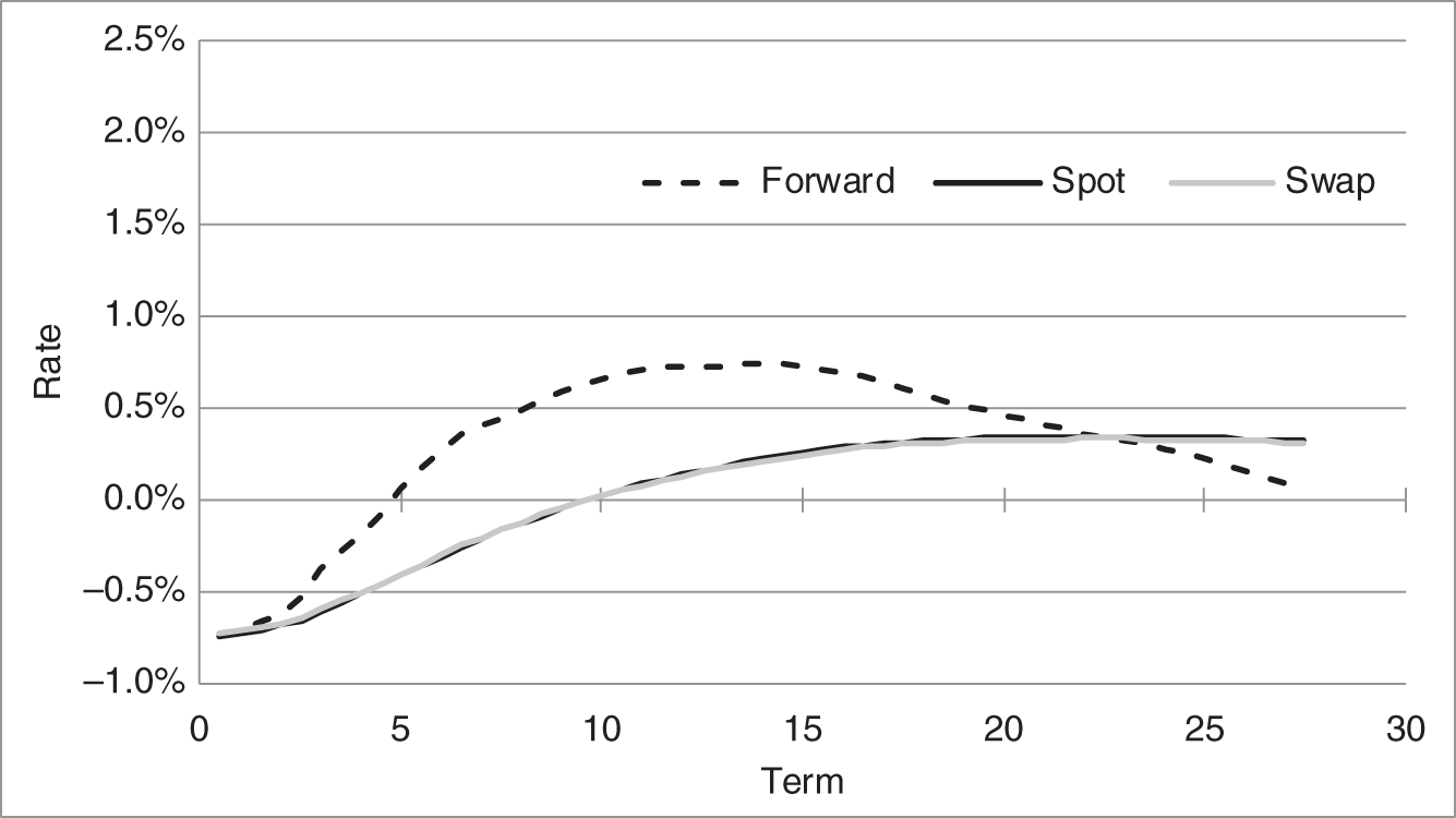
FIGURE 2.4 SARON Rate Curves, as of May 14, 2021.
The third and final relationship between rates to be highlighted in this section is the following: when spot rates are increasing with term, swap or par rates are slightly below spot rates. This effect can be seen in both Figures 2.3 and 2.4, though the effect is more noticeable for the SOFR than for the SARON curves. To understand the intuition here, recall that the ![]() ‐year spot rate is the return on an investment from today to year
‐year spot rate is the return on an investment from today to year ![]() , while the swap or par rate is the rate on an investment that pays every period from today to year
, while the swap or par rate is the rate on an investment that pays every period from today to year ![]() . The fair market swap rate, therefore, must reflect all of the spot rates from today to year
. The fair market swap rate, therefore, must reflect all of the spot rates from today to year ![]() , though the
, though the ![]() ‐year spot rate must be weighted most heavily as it is used to discount the by‐far‐and‐away largest cash flow, that is, the fictional notional amount. When the term structure of spot rates is upward‐sloping, then, all of the shorter‐term spot rates are lower than the
‐year spot rate must be weighted most heavily as it is used to discount the by‐far‐and‐away largest cash flow, that is, the fictional notional amount. When the term structure of spot rates is upward‐sloping, then, all of the shorter‐term spot rates are lower than the ![]() ‐year spot rate, and the
‐year spot rate, and the ![]() ‐year par rate – which reflects all those spot rates – must be less than the
‐year par rate – which reflects all those spot rates – must be less than the ![]() ‐year spot rate. But with the
‐year spot rate. But with the ![]() ‐year spot rate weighted particularly heavily, the par rate is not very much below that spot rate.
‐year spot rate weighted particularly heavily, the par rate is not very much below that spot rate.