
CHAPTER 8
Expectations, Risk Premium, Convexity, and the Shape of the Term Structure
Chapter 7 shows how bonds and other interest rate contingent claims can be priced given the evolution of the short‐term rate. This chapter shows how the shape of the term structure of interest rates is determined by assumptions about the evolution of the short‐term rate and by assumptions about the risk premium demanded by investors for bearing interest rate risk. The first few sections of the chapter present concepts by way of example, in the simple, binomial tree framework of the previous chapter. The last section of the chapter presents the same ideas in more general setting, though at the cost of some higher‐level mathematics. Chapter 9 concludes the presentation of term structure models with a detailed description of two well‐known models.
8.1 EXPECTATIONS
Consider a simple framework with annual periods. Assume for the moment that the current one‐year rate is 8%, and that investors know with certainty that the one‐year rate in one year will be 7% and in two years will be 6%. Then, the prices of one‐, two‐, and three‐year zero coupon bonds with a unit face value, ![]() ,
, ![]() , and
, and ![]() , are priced such that,
, are priced such that,

But by the definition of forward rates (see Chapter 2), Equations (8.1) say that the first three forward rates are 8%, 7%, and 6%. Hence, with investor certainty as to future interest rates, that is, without any volatility around those expectations, the term structure of interest rates – here expressed in terms of forward rates – is completely determined by expectations. Consequently, depending on expectations, the term structure can take on any shape: flat, upward‐sloping, downward‐sloping, or some combination of these.
In practice, expectations cannot sensibly take on any arbitrary pattern. The financial community can have very specific views about short‐term rates over short horizons, derived, for example, from anticipation of policy changes on central bank meeting dates and from the supply and demand conditions for funds (e.g., tax payment dates, the bond issuance calendar, quarterly balance sheet management). Over longer horizons, however, expectations are not as granular. Analysis of money market conditions is unlikely to reveal, for example, that the expected one‐year rate in 29 years is very different from the expected one‐year rate in 30 years. On the other hand, macroeconomic analysis might argue that the long‐run expectation of the short‐term rate is 4%: 1% due to the long‐run real‐rate of interest and 3% due to long‐run inflation.
8.2 VOLATILITY AND CONVEXITY
While investors have expectations about future short‐term rates, they recognize the limits of their analyses, that is, realized rates are assumed to fluctuate randomly around expectations. Continuing with the framework of the previous chapter, consider the binomial tree for the one‐year rate in the top part of Figure 8.1. The step size is one year, and the probabilities of all transitions are 50% (not shown). The level of rates and their volatility is exaggerated in this tree to illustrate the concepts of this chapter. Note that the expected value of the short‐term rate in one year is 9%, as is the expected short‐term rate in two years,
Note also that the volatility of the change in rate at any transition is 4%, or 400 basis points. For example, with the mean of the first transition calculated in Equation (8.2) to be 9%, the volatility of that transition is,
The price of a one‐year zero in this model is simply ![]() , or 0.917431. Assuming, for the moment, that investors are risk neutral, the price trees of the two‐ and three‐year zeros can be calculated by expected discounted value, as explained in the previous chapter. These trees are shown in the bottom of Figure 8.1, with the supporting calculations left to the reader. Table 8.1 collects the prices of the three zero coupon bonds, along with the associated forward rates. The striking feature of the table is that the term structure of forward rates is downward sloping, despite the fact that interest rate expectations are flat at 9%. This result can be explained by the interaction of interest rate volatility with the convexity of bond prices.
, or 0.917431. Assuming, for the moment, that investors are risk neutral, the price trees of the two‐ and three‐year zeros can be calculated by expected discounted value, as explained in the previous chapter. These trees are shown in the bottom of Figure 8.1, with the supporting calculations left to the reader. Table 8.1 collects the prices of the three zero coupon bonds, along with the associated forward rates. The striking feature of the table is that the term structure of forward rates is downward sloping, despite the fact that interest rate expectations are flat at 9%. This result can be explained by the interaction of interest rate volatility with the convexity of bond prices.
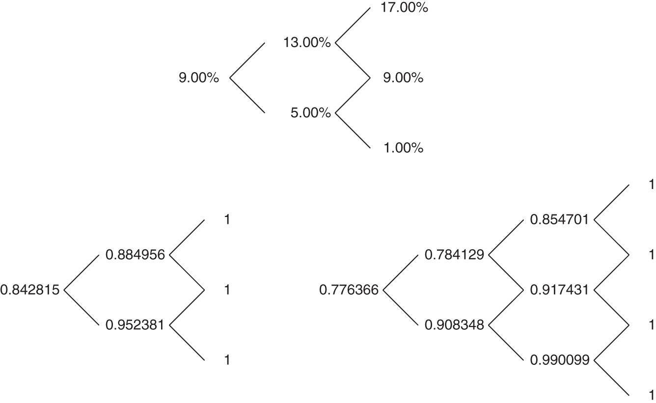
FIGURE 8.1 Binomial Rate Tree and Price Trees for Two‐ and Three‐Year Zero Coupon Bonds. Steps Are Annual, and the Probabilities of All Transitions Are 50%.
TABLE 8.1 Prices of Zero Coupon Bonds and Their Associated Forward Rates from the Rate Tree in Figure 8.1. Rates Are in Percent.
| Term | Price | Forward Rate |
|---|---|---|
| 1 | 0.917431 | 9.0000 |
| 2 | 0.842815 | 8.8532 |
| 3 | 0.776366 | 8.5590 |
A short detour is required at this point to present and explain Jensen's inequality as applied to bond pricing. For a random variable, like the one‐year rate, ![]() ,
,

In words, the expected price of a bond is greater than the price of a bond at the expected interest rate.
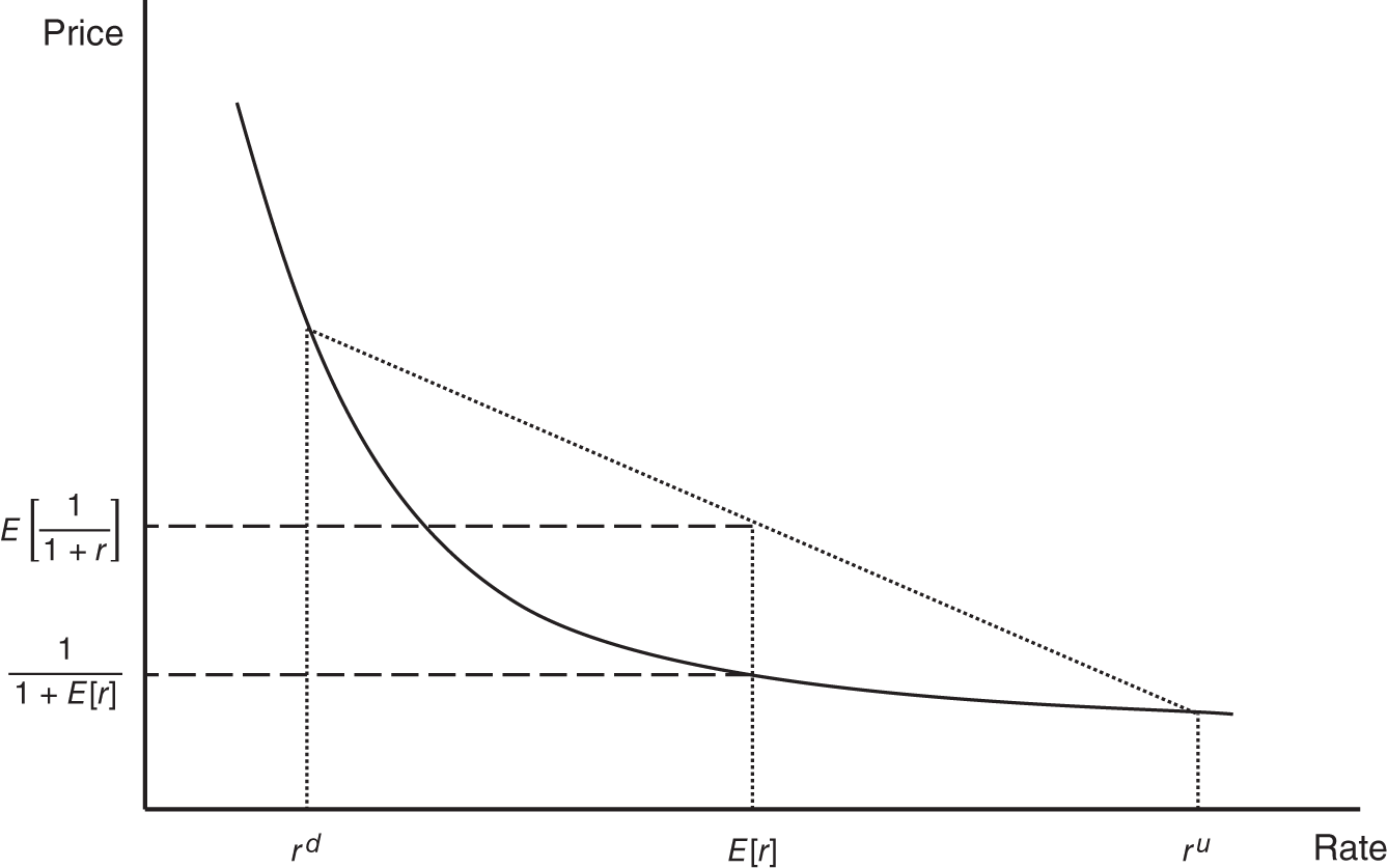
FIGURE 8.2 An Illustration of Jensen's Inequality as Applied to Bond Pricing.
This inequality is easily explained by Figure 8.2. In the figure, the rate can take on two values, ![]() and
and ![]() , with equal probability, resulting in an expected value just between them,
, with equal probability, resulting in an expected value just between them, ![]() . Each possible value of
. Each possible value of ![]() has an associated price, and the expected value of that price,
has an associated price, and the expected value of that price, ![]() , is graphically depicted as the vertical‐axis coordinate of the dotted line connecting the points
, is graphically depicted as the vertical‐axis coordinate of the dotted line connecting the points ![]() and
and ![]() . Because of the curvature or convexity of the price–rate curve, however, this expected price exceeds the price at a rate of
. Because of the curvature or convexity of the price–rate curve, however, this expected price exceeds the price at a rate of ![]() , which is
, which is ![]() . And this is exactly the relationship described in Equation (8.5).
. And this is exactly the relationship described in Equation (8.5).
Returning to the role of volatility and convexity, let ![]() denote the one‐year rate, one year forward, and consider the date‐0 price of a two‐year zero coupon bond, as expressed in Equation (8.6). By definition, the price of the two‐year zero equals its unit face amount discounted by 9% over the first year and by
denote the one‐year rate, one year forward, and consider the date‐0 price of a two‐year zero coupon bond, as expressed in Equation (8.6). By definition, the price of the two‐year zero equals its unit face amount discounted by 9% over the first year and by ![]() over the second year. By the logic of pricing along the tree, this price also equals the discounted expected value of the date‐1 price of the bond. Multiplying both sides of (8.6) by 1.09 and invoking Jensen's inequality in Equation (8.5), gives (8.7). And from this equation, (8.8) follows directly: the one‐year rate, one year forward, is less than the expected one‐year rate in one year,
over the second year. By the logic of pricing along the tree, this price also equals the discounted expected value of the date‐1 price of the bond. Multiplying both sides of (8.6) by 1.09 and invoking Jensen's inequality in Equation (8.5), gives (8.7). And from this equation, (8.8) follows directly: the one‐year rate, one year forward, is less than the expected one‐year rate in one year,


8.3 AN ANALYTICAL DECOMPOSITION OF FORWARD RATES
This section derives a general decomposition of forward rates in terms of expectations, convexity, and risk premium. The level of mathematics here is higher than used in most of the book, but the discussion still aims at intuition.
Assume that all bond prices are determined by the instantaneous rate, ![]() , which takes on the value of
, which takes on the value of ![]() at time
at time ![]() . Let
. Let ![]() be the price of a
be the price of a ![]() ‐year zero coupon bond at time
‐year zero coupon bond at time ![]() . By Ito's lemma, a discussion of which is beyond the scope of this book,
. By Ito's lemma, a discussion of which is beyond the scope of this book,

where ![]() ,
, ![]() , and
, and ![]() are the changes in price, rate, and time over the next instant, respectively, and
are the changes in price, rate, and time over the next instant, respectively, and ![]() is the volatility of changes in
is the volatility of changes in ![]() . The two first‐order partial derivatives in Equation (8.9) denote the instantaneous change in the bond price for a unit change in the rate (with time unchanged) and for a unit change in time (with rate unchanged), respectively. Finally, the second order partial derivative in the equation gives the instantaneous change in
. The two first‐order partial derivatives in Equation (8.9) denote the instantaneous change in the bond price for a unit change in the rate (with time unchanged) and for a unit change in time (with rate unchanged), respectively. Finally, the second order partial derivative in the equation gives the instantaneous change in ![]() (with time unchanged). Dividing both sides of (8.9) by price,
(with time unchanged). Dividing both sides of (8.9) by price,

Equation (8.10) breaks down the instantaneous return on the zero coupon bond into three components, but this decomposition can be written more intuitively by invoking several ideas from earlier chapters.
First, in terms of instantaneous compounded forward rates, ![]() , the price of a
, the price of a ![]() ‐year zero coupon bond is (from Section A2.1),
‐year zero coupon bond is (from Section A2.1),
Then, differentiating both sides of (8.11) with respect to ![]() , recognizing that increasing
, recognizing that increasing ![]() decreases
decreases ![]() one‐for‐one,
one‐for‐one,
Second, by the definitions of duration, ![]() , and convexity,
, and convexity, ![]() ,
,

Now, substituting Equations (8.12) through (8.14) into the return decomposition (8.10),
Equation (8.15) gives the return decomposition in terms of the following three components. The first is the return due to the passage of time, which, in this case, is the forward rate, ![]() .1 The second and third components are returns due to changes in the rate. The second term says that increases in rate reduce bond return in proportion to duration. The third term says that the volatility of rates – movement of rates either up or down – increases return in proportion to convexity. To appreciate this term, recall from Chapter 4 that, across portfolios with the same duration, more convex portfolios increase more in value as rates change (at a fixed moment in time), whether rates rise or fall.
.1 The second and third components are returns due to changes in the rate. The second term says that increases in rate reduce bond return in proportion to duration. The third term says that the volatility of rates – movement of rates either up or down – increases return in proportion to convexity. To appreciate this term, recall from Chapter 4 that, across portfolios with the same duration, more convex portfolios increase more in value as rates change (at a fixed moment in time), whether rates rise or fall.
To draw conclusions about expected returns, take the expectation of both sides of (8.15),
The intuition of this decomposition is the same as for Equation (8.15), but with the duration component depending not on the change in rate but on the expected change in rate.
The next step in the analysis introduces the concept of a risk premium. Risk‐neutral investors, who do not require a risk premium, demand that each bond offer an expected return equal to the short‐term rate of interest. Mathematically,

Risk averse investors, however, demand higher expected returns for bonds with greater interest rate risk. The appendix to this chapter shows that the interest rate risk of a bond over the next instant may be measured by its duration with respect to the interest rate factor, and that risk‐averse investors demand a risk premium proportional to duration. This risk premium may depend on time and on the level of rates, but not on the characteristics of any individual bond. The discussion proceeds here, however, as if the risk premium were constant and denoted by ![]() . In that case, the expected return equation for risk‐averse investors is,
. In that case, the expected return equation for risk‐averse investors is,

Say, for example, that the short‐term rate is 1%, that the duration of a bond is five, and that the risk premium is 10 basis points per year of duration risk. Then, according to Equation (8.18), the bond's expected return is ![]() per year.
per year.
Another useful way to think of the risk premium is in terms of the Sharpe ratio (SR) of a security, defined as its expected excess return (over the short‐term rate) divided by the standard deviation of its return. Because the random part of a bond's return comes from its duration times the change in rate, as in Equation (8.15), the standard deviation of the return equals the duration times the standard deviation of rates. Therefore, the SR of a bond may be written as,

where the second equality follows from Equation (8.18). For example, if the risk premium is 10 basis points per year, and if the standard deviation of rates is 100 basis points per year, then the Sharpe ratio of bond investments is 10%.
The decomposition of returns can now be combined with the economics of the risk premium to draw conclusions about the shape of the term structure of forward rates. Equating the expressions for expected returns in the right‐hand sides of Equations (8.16) and (8.18),

Equation (8.20) mathematically describes the determinants of forward rates. The three terms represent the impacts of expectations, risk premium, and convexity, respectively. The first term says that the forward rate is composed of the instantaneous interest rate plus the expected change in that rate times the duration of the zero coupon bond corresponding to the term of the forward rate. In other words, the higher the instantaneous rate, the higher the forward rate; the more rates are expected to increase, the higher the forward rate; and the greater the corresponding duration, the greater the effect of expected rate changes on the forward rate.
The second term on the right‐hand side of (8.20) says that the forward rate increases with the risk premium in proportion to the corresponding duration. In other words, the greater the corresponding interest rate risk and the greater the risk premium, the greater the forward rate.
Chapter 7 noted that a drift in the short‐term rate of a certain number of basis points has the same effect on bond pricing as a risk premium of that number of basis points per year of duration risk. Equation (8.20) formalizes this statement. Increasing the risk premium or increasing the expected short‐term rate by the same amount are indistinguishable from the observation of forward rates. This means that the term structure of interest rates cannot, on its own, be used to separate expectations of rate changes from risk premium. From a modeling perspective, this means that only the risk‐neutral process is relevant for pricing. Dividing the risk‐neutral drift into expectations and risk premium might be very useful for economic perspectives and for macro‐style trading (see Chapter 9), but this division is not observable from a cross section of bond prices alone.
The first two terms of Equation (8.20) can also be cast in terms of theories of the term structure of interest rates. (Put aside the convexity term for the moment.) Under the pure expectations hypothesis, the risk premium, ![]() , is zero, and the term structure of forward rates is determined by expectations,
, is zero, and the term structure of forward rates is determined by expectations, ![]() . In this view of the world, the most natural “no‐change” scenario, in the terms of Chapter 3, is that short‐term rates evolve as expected and that forward rates are realized. At the opposite extreme, under the pure risk premium hypothesis, the market has no expectations about rates, that is,
. In this view of the world, the most natural “no‐change” scenario, in the terms of Chapter 3, is that short‐term rates evolve as expected and that forward rates are realized. At the opposite extreme, under the pure risk premium hypothesis, the market has no expectations about rates, that is, ![]() , and the term structure of forward rates is determined by the risk premium. In this view of the world, the most natural “no‐change” scenario is that short‐term rates stay the same, as expected, which, in terms of Chapter 3 is an unchanged term structure. The reality, of course, can be between the two extremes, such the the term structure is determined by a mix of expectations and risk premium.
, and the term structure of forward rates is determined by the risk premium. In this view of the world, the most natural “no‐change” scenario is that short‐term rates stay the same, as expected, which, in terms of Chapter 3 is an unchanged term structure. The reality, of course, can be between the two extremes, such the the term structure is determined by a mix of expectations and risk premium.
To conclude the discussion of Equation (8.20), the third term shows that the forward rate is reduced because of volatility and the convexity of the zero corresponding to the term of the forward rate by ![]() . Using this to reinterpret Equation (8.16), the indirect reduction in return through the forward rate, because of convexity, is exactly offset by the direct increase in return, because of convexity. Put another way, the expected return condition of Equation (8.18) ensures that there is no net advantage of convexity. The significance of this reasoning for investment and hedging decisions is introduced in Chapter 4 in the context of establishing long‐ and short‐convexity positions.
. Using this to reinterpret Equation (8.16), the indirect reduction in return through the forward rate, because of convexity, is exactly offset by the direct increase in return, because of convexity. Put another way, the expected return condition of Equation (8.18) ensures that there is no net advantage of convexity. The significance of this reasoning for investment and hedging decisions is introduced in Chapter 4 in the context of establishing long‐ and short‐convexity positions.