
CHAPTER 3
Returns, Yields, Spreads, and P&L Attribution
Chapter 2 showed how swap or par rates, spot rates, and forward rates are used to describe the interest rates that can be earned in various markets, like the Treasury bond market or the interest rate swap market. While these rates are derived from the prices of individual financial instruments, they are intended to describe the time value of money in a market as a whole. This chapter, by contrast, focuses on rates that are specific to individual bonds and then uses both market‐wide and security‐specific rates for P&L (profit and loss) attribution.
The first section of the chapter defines the realized return on a bond over a given horizon. Ex‐post bond returns have to account for interim coupon payments and the reinvestment of those payments and are often computed on both a gross basis and net of financing, but are otherwise calculated like the returns on any other asset.
The next sections present yield to maturity. Bonds are often quoted and traded in terms of yield rather than price; yields are widely thought of as indicative of ex‐post returns; and differences in bond yields are commonly regarded as indicative of differences in value. The discussion reveals, however, that yields can be misleading with respect to both ex‐post returns and relative values.
The chapter continues with bond spreads. Because there are so many related but distinct fixed income products, spreads are used to quote, trade, and value one instrument relative to another. This part of the chapter describes various ways to compute spreads, explains their uses and limitations, and presents a detailed example of using spreads to assess the relative value of high‐coupon US Treasury bonds.
The last sections of the chapter are devoted to attribution. In order to understand the performance of their trades and investments, traders and asset managers often divide their ex‐post P&L or return into various components, for example, the passage of time; changing interest rates; and changing spreads. The text describes how to define the “passage of time,” holding rates or spreads constant, and then illustrates P&L attribution with a detailed example of breaking into components the return on a particular US Treasury bond.
3.1 REALIZED RETURNS
The gross horizon return of a bond depends on the price at which the bond was bought; the coupon payments it earns over the horizon; the interest on the reinvestment of those coupon payments over the horizon; and the price of the bond at the end of the horizon. The net horizon return of the bond adjusts its gross return for the cost of financing its purchase.
Begin with a simple example. An investor buys $1 million face amount of the US 7.625s of 11/15/2022 at 114.8765 in mid‐November 2020. Six months later, in mid‐May 2021, the price of the bond is 111.3969.1 The gross return of the bond over the horizon is, therefore,

In words, the six‐month holding period return in this example equals the value of the bonds at the end of the six months, or $1,113,969; plus the coupon payment at that time of half 7.625% on the $1 million face amount, or $38,125; minus the initial cost of the bonds, or $1,148,765, all divided by that initial cost. Note that the coupon income of the bond is sufficient to overcome the fall in price and result in a positive horizon return.
Realized return over a horizon that extends past a coupon payment depends on the rate at which coupon payments have been reinvested. If a bond makes a coupon payment in one month, but the horizon is two months, the horizon return depends on the one‐month reinvestment rate, from the coupon payment date to the end of the horizon. For the purposes of illustration, consider the simple case of an investment in the 7.625s of 11/15/2022 over a horizon of one year. If the price of the bond at the end of the year is $1,080,000, and if the coupon payment of $38,125 after six months is reinvested for the subsequent six months at a money market rate of, say, 0.05%, then the realized return of the investment over the year is,

The discussion now turns to the return net of the cost of financing the purchase of a bond. This might be an explicit cost; that is, a trader or investor might borrow the purchase price of the bond for six months at an interest rate of 0.05%. In that case, the interest cost of the borrowing over the investment horizon, ![]() , would be subtracted from the numerator of Equation (3.1) to give a return net of financing of,
, would be subtracted from the numerator of Equation (3.1) to give a return net of financing of,

Not surprisingly, the net return of 0.2648% is the gross return, 0.2898%, minus the half‐year borrowing cost of ![]() , or 0.025%.
, or 0.025%.
There are actually several subtleties in describing the net return on a bond investment in this way. First, market participants do fund bond purchases using the purchased bonds as collateral in the repurchase or repo market, which is the subject of Chapter 10. Second, only a portion of the purchase price can typically be funded in this market. In the present case, for example, an investor might be able to borrow only $1,125,790, or only 98%, of the total purchase price. In this case, the interest cost would only be half of 0.05% on that $1,125,790, or $281, and the net return would be 0.2653%, which is very slightly higher than the result from Equation (3.3). Third, regardless of how much is actually borrowed, the net return is calculated with the total purchase price as the denominator of (3.3). This formulation of net return, therefore, can be thought of as a return on balance sheet, that is, on the value that can be considered and reported as an asset. Fourth, return on capital would be computed differently. If a hedge fund borrows 98% of the value of the bond in the repo market, while putting up 2%, or $22,975 of its own capital, then this investment's return on capital – abstracting from any additional allocations of risk capital to the trade – would be,

The 13.27% return on capital is 50 times the net balance sheet return of 0.2653%. This high return on capital is due to the fact that the trade, as described, has a leverage of 50, that is, an asset value of $1,148,765 purchased with capital of only $22,975.
The fifth and final subtlety with respect to net returns is that financing costs should most likely be considered even without any explicit repo borrowing. Any money used to purchase a bond had to have been raised at some cost (e.g., a bank paying money to attract deposits; a life insurance company compensating investors for the savings portions of their policies; a hedge fund offering a return on its assets under management). Furthermore, any money invested in a particular bond has an opportunity cost in the sense that this money might have been used to fund a different investment.
3.2 YIELD TO MATURITY
Chapter 2 made the point that rates are often more intuitive than prices in describing bond valuation. But, along the lines of that chapter, to describe the pricing of a 10‐year bond in terms of semiannually compounded spot rates or forward rates requires 20 of those spot or forward rates. It is hardly surprising, therefore, that market participants prefer to quote the price of a bond and to think about its valuation with a single rate, namely, its yield to maturity.
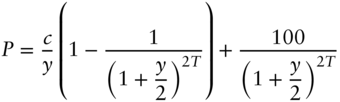
The yield to maturity of a bond is the single rate such that discounting the bond's cash flows by that rate gives the bond's market price. Table 1.4 reported the price of the US Treasury 7.625s of 11/15/2022 for settlement in mid‐May 2021 as 111.3969. Recalling that US Treasury bonds pay coupons semiannually so that this bond had three remaining payment dates, and noting the Treasury bonds are quoted with semiannually compounded yields, the yield to maturity of this bond, ![]() , is defined as,2
, is defined as,2

Equation (3.5) can be solved for ![]() by some numerical method or with a financial calculator, giving a result of 0.0252%. Hence, trades of this bond could be quoted and consummated either at a price of 111.3969 or at a yield of 0.0252%.
by some numerical method or with a financial calculator, giving a result of 0.0252%. Hence, trades of this bond could be quoted and consummated either at a price of 111.3969 or at a yield of 0.0252%.
More generally, let ![]() denote the yield of a bond; let
denote the yield of a bond; let ![]() denote its annual, dollar coupon payment; let
denote its annual, dollar coupon payment; let ![]() denote its maturity in years, which means there are
denote its maturity in years, which means there are ![]() semiannual payments remaining; and let
semiannual payments remaining; and let ![]() denote its price, per 100 face amount, for settlement on a coupon payment date. To illustrate notation, note that for the 7.625s of 11/15/2022 settling in mid‐May 2021,
denote its price, per 100 face amount, for settlement on a coupon payment date. To illustrate notation, note that for the 7.625s of 11/15/2022 settling in mid‐May 2021, ![]() ,
, ![]() ,
, ![]() , and
, and ![]() . Returning to the general case, then,
. Returning to the general case, then, ![]() is given by,
is given by,


where Equation (3.7) just re‐expresses (3.6) with summation notation, and Equation (3.8) follows from (3.7) and Equation (A2.16) of Appendix A2.2.
Equation (3.8) reveals three immediate implications about the price–yield relationship. First, when ![]() ,
, ![]() : when the coupon payment is the face amount times the yield, or, more simply, when the coupon rate equals the yield, the bonds sells for its face amount, or par. Second, when
: when the coupon payment is the face amount times the yield, or, more simply, when the coupon rate equals the yield, the bonds sells for its face amount, or par. Second, when ![]() ,
, ![]() : when the coupon rate exceeds the yield, the bond sells at a premium to par. Third, when
: when the coupon rate exceeds the yield, the bond sells at a premium to par. Third, when ![]() ,
, ![]() : when the yield exceeds the coupon rate, the bond sells at a discount to par.
: when the yield exceeds the coupon rate, the bond sells at a discount to par.
Figure 3.1 illustrates the relationship between price and yield as described by Equations (3.6) to (3.8). Every point along the curves in the figure represents a bond with a particular coupon and maturity, and all bonds in the figure are priced at a yield of 1.5%. The thick black line, then, shows that bonds with a coupon rate of 1.5%, of any maturity, have a price of 100. Investors are willing to pay 100 for a bond that pays the going market coupon rate over time and then returns par at maturity.
Bonds with a coupon rate greater than the fixed yield of 1.5%, represented by the 3% and 6% gray, dashed lines in the figure, sell at a premium to par. With 30 years to maturity, the price a 6% bond yielding 1.5% is about 208, while the price of a 3% bond at that yield is about 136. Investors are willing to pay much more than par for these bonds because they pay above‐market coupon rates for many years. Bonds with the same coupon rates but shorter maturities still command premiums, but smaller ones. For example, the prices of the 15‐year bonds in the figure with 6% and 3% coupon rates are about 160 and 120, respectively. And, as maturities get very short, prices approach 100: while the 6% and 3% bonds do pay above‐market coupon rates, they do so for such a short time that their prices are not much above 100.

FIGURE 3.1 Prices of Bonds with Different Coupons and Maturities. All Yields Equal 1.5%.
Following similar reasoning, the lines in Figure 3.1 representing bonds with coupon rates of 0% and 0.75% show prices all below par. The discount is greatest for the longest maturity bonds, for which investors receive below‐market coupon rates for the longest times, with the prices of 30‐year 0% and 0.75% bonds being about 64 and 82, respectively. Price is less discounted for shorter maturity bonds, to about 80 and 90 at 15 years, respectively, until bonds very near maturity sell for just under par. The trend of premium and discount bond prices to approach par as they mature is known as the pull to par. This behavior, of course, is only the trend, at a fixed yield of 1.5%. The actual price paths of these bonds as they mature are determined by their realized market yields.
3.3 YIELD AND RETURN
As mentioned earlier, yield to maturity is a convenient way to express price in terms of a single rate of interest. And the definition of yield as the single rate that equates the present value of a bond's cash flows to its price means that yield is a bond's internal rate of return. But how does yield relate to a bond's realized return?
As it turns out, yield is only weakly related to realized returns. Appendix A3.2 shows that a bond's ex‐post return is equal to its initial yield if i) all of the coupons are reinvested at the initial yield, and ii) if the yield at the end of the investment horizon is the same as the initial yield. These very restrictive conditions significantly weaken the interpretation of yield as a predictor of holding period return.
To demonstrate this point with a concrete example, consider the return on the 7.625s of 11/15/2022 from mid‐May 2021 to mid‐May 2022. Begin with Equation (3.5), which gives that bond's yield as of the start of that period, and multiply both sides by ![]() ,
,

The left‐hand side is the proceeds from an investment of the price of the bond, 111.3969, for one year – or two semiannual periods – at the semiannually compounded rate ![]() . The right‐hand side is the value of the bond position at the end of the one‐year horizon, which is the sum of three parts: the proceeds from the first coupon, received on November 15, 2021, and invested for six months to May 15, 2022; the coupon received on May 15, 2022; and the price of the bond on May 15, 2022, if its yield is
. The right‐hand side is the value of the bond position at the end of the one‐year horizon, which is the sum of three parts: the proceeds from the first coupon, received on November 15, 2021, and invested for six months to May 15, 2022; the coupon received on May 15, 2022; and the price of the bond on May 15, 2022, if its yield is ![]() . In words then, Equation (3.9) says that the one‐year return on the initial investment will be
. In words then, Equation (3.9) says that the one‐year return on the initial investment will be ![]() if the first coupon is reinvested at
if the first coupon is reinvested at ![]() and if the bond, at the end of the year, is priced at a yield of
and if the bond, at the end of the year, is priced at a yield of ![]() . If
. If ![]() in every term of (3.9) is the initial yield of the bond, that is, 0.0252%, then the bond earns that initial yield over the year. But if the coupon reinvestment rate or the yield of the bond at the end of year have changed over time, and are not equal to 0.0252%, then the bond likely does not earn that rate over the one‐year horizon.
in every term of (3.9) is the initial yield of the bond, that is, 0.0252%, then the bond earns that initial yield over the year. But if the coupon reinvestment rate or the yield of the bond at the end of year have changed over time, and are not equal to 0.0252%, then the bond likely does not earn that rate over the one‐year horizon.
To see that a bond may not earn its initial yield even if held to maturity, multiply both sides of Equation (3.5) by ![]() to get,
to get,
Now, the left‐hand side is the proceeds from an investment of 111.3969 for 1.5 years. The right‐hand side is the value of the bond position at maturity, that is, November 15, 2022, which is, again, the sum of reinvested coupons and the final coupon and principal payments. If ![]() in every term of (3.10) is the initial yield, then the bond earns that initial yield to maturity. But if coupons are invested at a different rate, the bond does not earn its initial yield over its life.
in every term of (3.10) is the initial yield, then the bond earns that initial yield to maturity. But if coupons are invested at a different rate, the bond does not earn its initial yield over its life.
The 7.625s of 11/15/2022 are useful in making the point that yield does not coincide with horizon return, but its short maturity, along with its low yield, may give a misleading impression of orders of magnitude. Consider, therefore, buying the US Treasury 2.375s of 5/15/2051 in mid‐May 2021, at a price of 100.6875 or yield of 2.343%, and holding it to maturity. Along the lines of the previous paragraphs, if all coupons are reinvested at 2.343%, then the return on the initial investment over the 30 years is 2.343% per year. But if rates were to fall suddenly and remain low, so that all coupons are invested at 0%, or if the investor holds all coupon payments in a non‐interest‐bearing account, the return on the bond to maturity falls to 1.778% per year. If, on the other hand, rates were to rise suddenly and remain high, so that all coupons were reinvested at 5%, then the bond return rises to 3.207% per year. Reproducing these results is left as an exercise to the reader.
3.4 YIELD AND RELATIVE VALUE
This section argues that yield is not a reliable measure of relative value. In fact, if two bonds have the same maturity but different yields, it is not necessarily true that the bond with a higher yield is a superior investment. To explain this, the discussion turns to the coupon effect, starting with a simple numerical example and finishing with an empirical demonstration from the US Treasury bond market.
Say that the one‐year spot rate is 0% and the two‐year spot rate is 10%. Using the analytics of Chapter 2 and of this chapter, Table 3.1 gives the prices and yields of three two‐year bonds with annual coupons of 0%, 5%, and 9.5023%.
For example, for the 5% bond,


where Equation (3.11) uses the assumed spot rates to discount cash flows and Equation (3.12) follows from the definition of yield to maturity.
According to Table 3.1, the yield of the zero coupon bond is 10%. Because this bond makes only one payment at maturity, its market price can be found by discounting at either the two‐year spot rate or at the bond's yield. Hence, those two must be equal at 10%.
TABLE 3.1 Prices and Yields of Two‐Year Bonds When the One‐ and Two‐Year Spot Rates are 0% and 10%, Respectively. Coupons and Yields Are in Percent.
| Coupon | Price | Yield |
|---|---|---|
| 0.0000 | 82.6446 | 10.0000 |
| 5.0000 | 91.7769 | 9.7203 |
| 9.5023 | 100.0000 | 9.5023 |
The yield of the 5% bond, however, is 9.7203%. Equations (3.11) and (3.12) show that the yield of 9.7203% has to summarize the term structure of spot rates, or, in other words, that discounting at the yield has to have the same effect as discounting the first cash flow by 0% and the second by 10%. The result of 9.7203% is between the two spot rates, but a lot closer to 10%: most of the bond's cash flow comes from the second payment, which includes principal, and that second payment is discounted at 10%.
Table 3.1 also reports that the 9.5023% bond, which sells for par, has a yield of 9.5023%. This yield is also between the spot rates of 0% and 10%, and is also a lot closer to 10% but not as close as for the 5% bond. Because the 9.5023% bond pays out relatively more of its value in the first cash flow, its yield is closer to 0% than is the yield of the 5% bond.
In general, the coupon effect can be summarized as follows: when the term structure of spot rates is upward sloping, bonds with higher coupons, which have more of their value discounted at shorter‐term, lower spot rates, have lower yields to maturity. While not part of the discussion here, it is also true that when the term structure of spot rates is downward sloping, bonds with higher coupons have higher yields.
The coupon effect makes it very clear that spot rates are meant to describe pricing in a bond market as a whole, while yields are meant to describe the pricing of individual bonds. Furthermore, even though all of the bonds in the table are fairly priced relative to the term structure of spot rates, each bond has a different yield. Put another way, the fact that the 0% bond has the highest yield does not mean that it is the best investment. The fact that the par bond has the lowest yield does not mean that it is the worst investment.
Figures 3.2 and 3.3 show the coupon effect at work in the US Treasury market as of mid‐May 2021. Figure 3.2 graphs the yields of all Treasury coupon bonds against their maturity dates. Some bond yields are clearly off the curve. The four points above the curve with maturities from 2040 to 2041 are relatively newly issued 20‐year bonds. The Treasury stopped issuing new 20‐year bonds in 1986 but started to do so again in May 2020. These four bonds, therefore, have coupons that reflect the current, low‐rate environment. The other outstanding bonds with similar maturities were originally issued about 10 years ago as 30‐year bonds, and, therefore, have relatively high coupons, which reflect the interest rate environment at the time they were issued.
Table 3.2 shows the coupons and yields of these four newly issued 20‐year bonds, each paired with the coupons and yields of old 30‐year bonds of the same maturity. As expected, because of the coupon effect and the upward‐sloping term structure of rates, the high‐coupon, old 30‐year bonds have lower yields than the low‐coupon, newly issued 20‐year bonds. More analysis is needed, of course, to say that any one bond in this table is cheap or rich relative to another. But, because of the coupon effect, the fact that the new 20‐year bonds have higher yields does not necessarily imply that they are better investments.
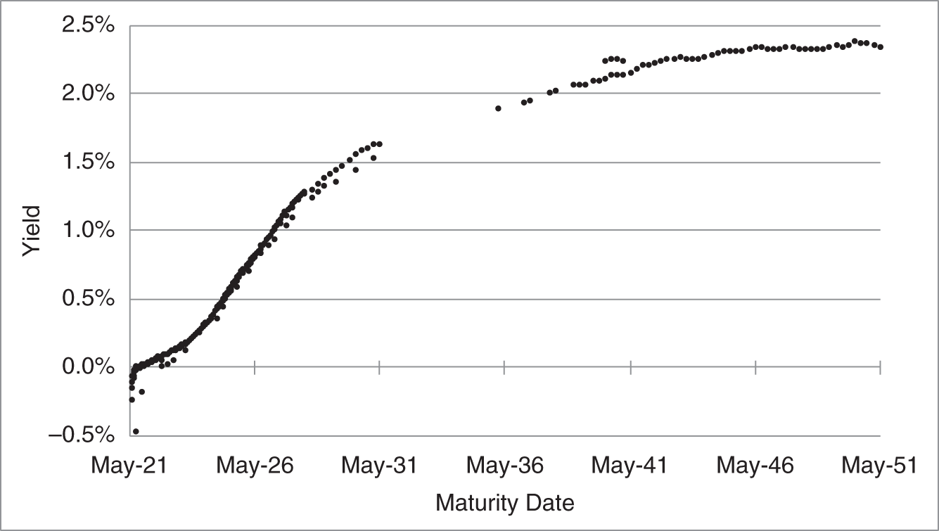
FIGURE 3.2 Yields of US Treasury Bonds, as of May 14, 2021.
TABLE 3.2 Yields of Selected US Treasury Bonds Maturing Between May 15, 2040, and February 15, 2041, as of May 14, 2021. Coupons and Yields Are in Percent.
| New 20‐Year Bonds | Old 30‐Year Bonds | |||
|---|---|---|---|---|
| Maturity | Coupon | Yield | Coupon | Yield |
| 05/15/2040 | 1.125 | 2.237 | 4.375 | 2.107 |
| 08/15/2040 | 1.125 | 2.245 | 3.875 | 2.138 |
| 11/15/2040 | 1.375 | 2.245 | 4.250 | 2.140 |
| 02/15/2041 | 1.875 | 2.236 | 4.750 | 2.133 |
Returning to Figure 3.2, there are several bonds that mature on or before May 2031 that have yields noticeably below the curve.3 To examine these bonds, Figure 3.3 zooms in on maturities on or before May 2031. The dots represent bonds with coupon rates less than or equal to 5%, while the plus signs represent bonds with coupon rates greater or equal to 5.25%. Once again, as expected because of the coupon effect and the upward‐sloping term structure, the bonds with the higher coupons have lower yields.

FIGURE 3.3 Yields of US Treasury Bonds Maturing in Less than 10 Years, as of May 14, 2021.
3.5 SPREADS
There are many fixed income securities. Their prices all depend in some way on market‐wide interest rates, but also on idiosyncratic factors, like credit risk, tax treatment, and unique supply and demand considerations. To make sense of pricing in this context, market participants often quote spreads of one instrument or set of instruments relative to others.
Consider the European sovereign debt market. Because the market perceives the credit characteristics of each country's bond issues differently, some countries typically pay higher interest rates on their bonds than other countries. These differences could be described by comparing individual prices and yield. As of May 2021, for example, the Italian government bond or BTP (Buoni del Tesoro Poliennali) 0.60s of 08/1/2031 (issued in February 2021) sold at a price of 95.502, or a yield of 1.066%. At the same time, the German government bond or Bund 0.00s of 02/15/2031 (issued in January 2021) sold at a price of 101.300, or a yield of ![]() 0.132%. Market participants often find it more intuitive, however, to describe the market by saying that the 10‐year BTP‐Bund spread – in this case just the difference between the two yields – is 1.198%, or about 120 basis points. Note that one basis point is defined as 0.01%, so that 120 basis points is 1.20%. In any case, spreads of government bonds in many countries are often quoted against a Bund benchmark because Germany is widely regarded as having the strongest credit in the region.
0.132%. Market participants often find it more intuitive, however, to describe the market by saying that the 10‐year BTP‐Bund spread – in this case just the difference between the two yields – is 1.198%, or about 120 basis points. Note that one basis point is defined as 0.01%, so that 120 basis points is 1.20%. In any case, spreads of government bonds in many countries are often quoted against a Bund benchmark because Germany is widely regarded as having the strongest credit in the region.
Yield spreads can also be convenient for trading bonds that are less liquid than benchmark bonds. For example, in August 2020, Johnson & Johnson (JNJ) issued a number of long‐term bonds, including its 20‐year 2.10s due 09/1/2040. The pricing of this new issue was quoted as 75 basis points above the on‐the‐run 30‐year Treasury bond, the 1.25s of 05/15/2050. Quoting yield against a Treasury benchmark is not only intuitive, but also facilitates trading in fast‐moving markets. A fixed yield spread over a liquid Treasury bond allows the offering price of the JNJ bond to change smoothly and predictably with market levels until the new issue is actually sold.
While yield spreads are particularly easy to calculate and use, they are actually difficult to interpret carefully for two reasons. First, in many situations there is no liquid, benchmark bond with exactly the same maturity as the less‐liquid bond. Taking the differences in yields, therefore, mixes differences in term with other differences, like credit. In the 20‐year JNJ issue, for example, the spread of 75 basis points includes not only the credit risk of JNJ relative to the US Treasury, but also the difference between 20‐ and 30‐year yields. Second, spreads of yields, even of the same maturity, inherit the weakness of yield described earlier and expressed as the coupon effect. Put another way, the yield spread between bonds of the same maturity can be misleading if their coupons are different and their underlying term structures have different shapes.
Bond spreads are a more careful and more meaningful formulation of expressing price differences as a spread of rates.4 To illustrate, consider again the US Treasury 7.625s of 11/15/2022. Table 1.3 derives discount factors from a set of newly issued, benchmark Treasury bonds, which did not include the 7.625s of 11/15/2022. Table 1.4 then shows that the 111.3969 market price of the 7.625s of 11/15/2022 is 11.72 cents rich relative to its 111.2797 present value, which is computed using the discount factors derived from the benchmark bonds. The point of a bond spread is to express this 11.72 cents of richness as a spread of rates. Bond spreads can be computed relative to par, spot, or forward rates, but this section works with forward rates. The forward rates implied from the discount factors in Table 1.3 are 0.0154%, 0.1008%, and 0.1833%, for terms of 0.5, 1.0, and 1.5 years, respectively. Therefore, the 111.2797 present value of the 7.625s of 11/15/2022 is given by,

The bond spread with respect to forward rates is defined as the spread that, when added to each forward rate, sets the bond's present value equal to its market price. In this case, denoting the spread by ![]() ,
,

Solving, ![]() , or about minus seven basis points. The spread is negative because the bond is rich; that is, the market price is above the present value as computed with the benchmark curve. In other words, the benchmark forward curve has to be shifted down to recover the relatively high market price.5
, or about minus seven basis points. The spread is negative because the bond is rich; that is, the market price is above the present value as computed with the benchmark curve. In other words, the benchmark forward curve has to be shifted down to recover the relatively high market price.5
A bond's spread can be interpreted as its extra return, relative to the benchmark bonds, if rates “stay the same,” or if interest rate risk is hedged away. This interpretation is developed in the next section and in Chapter 7.
Because bond spread can be interpreted as an indicator of relative value, many practitioners routinely compute bond spreads, whether it be spreads of various European government bonds to German Bunds, spreads of corporate bonds to government bonds or swaps, spreads of government bonds to benchmark government bonds, or even spreads of government bonds to swaps. With respect to the last of these, it had once been standard to compute spreads of government bonds only to the most liquid government bonds. But as LIBOR swaps became more and more liquid, and as the idiosyncratic pricing of individual government bonds became more apparent, market participants began to compute spreads of government bonds to LIBOR swaps as well. SOFR swaps, which are now replacing LIBOR swaps, may take on the same role in the future.
3.6 APPLICATION: SPREADS OF HIGH‐COUPON TREASURIES
To illustrate the use of bond spreads in assessing relative value, the top panel of Table 3.3 and the gray lines in Figure 3.4 report the bond spreads of selected Treasury bonds relative to benchmark Treasury bonds and also relative to SOFR swaps. The benchmark Treasuries, by definition, have zero spreads relative to themselves. Consistent with the analysis of high‐coupon bonds in terms of the law of one price in Chapter 1, high‐coupon bonds are rich relative to benchmark Treasuries, with bond spreads ranging from ![]() 0.8 to
0.8 to ![]() 18.9 basis points. Traders and investors can use these spreads in their investment decisions. Because these bonds are rich, buying them sacrifices return relative to buying benchmark bonds, implying that there needs to be some reason, not considered here, to purchase these bonds. Conversely, because these bonds are rich, selling or shorting them picks up return relative to benchmark bonds, absent some factor not considered in this analysis.
18.9 basis points. Traders and investors can use these spreads in their investment decisions. Because these bonds are rich, buying them sacrifices return relative to buying benchmark bonds, implying that there needs to be some reason, not considered here, to purchase these bonds. Conversely, because these bonds are rich, selling or shorting them picks up return relative to benchmark bonds, absent some factor not considered in this analysis.
As mentioned already, market practitioners sometimes use swaps as a benchmark against which to compute government bond spreads. For the bonds in this example, spreads to SOFR swaps are reported in the bottom panel of Table 3.3 and with the black lines in Figure 3.4. With respect to the relative pricing of high‐coupon bonds, the SOFR spreads tell the same story as the Treasury spreads: high‐coupon bonds have lower (and more negative) spreads and, therefore, are rich to benchmark Treasury bonds. In fact, the differences between the spreads of high‐coupon bonds and of benchmark bonds are about the same whether measured against benchmark bonds or SOFR swaps. With respect to relative pricing across term, however, the results are quite different. Measured against SOFR swaps, longer‐term bonds – both high‐coupon and benchmark – are much cheaper than shorter‐term bonds. Consider, for example, the spreads of the 5.25s of 11/15/2028 and the 8s of 11/15/2021. The difference in their SOFR spreads is ![]() or 44.3 basis points, while the difference in their Treasury spreads is
or 44.3 basis points, while the difference in their Treasury spreads is ![]() or only 16.8 basis points. And the difference in SOFR spreads between the 3.125s of 11/15/2028 and the 2.875s of 11/15/2021 is
or only 16.8 basis points. And the difference in SOFR spreads between the 3.125s of 11/15/2028 and the 2.875s of 11/15/2021 is ![]() or 28.3 basis points, while the difference in their Treasury spreads, because they are both benchmark bonds, is, by definition, zero. Hence, longer‐term bonds look much cheaper relative to short‐term bonds when measured against SOFR than against Treasuries.
or 28.3 basis points, while the difference in their Treasury spreads, because they are both benchmark bonds, is, by definition, zero. Hence, longer‐term bonds look much cheaper relative to short‐term bonds when measured against SOFR than against Treasuries.
TABLE 3.3 Spreads of Selected US Treasury Bonds to Benchmark Treasuries and to SOFR Swaps, as of May 14, 2021. Coupons Are in Percent, and Spreads Are in Basis Points.
| Benchmark Treasuries | High‐Coupon Treasuries | |||
|---|---|---|---|---|
| Maturity | Coupon | Spread | Coupon | Spread |
| Spreads to Benchmark Treasuries | ||||
| 11/15/2021 | 2.875 | 0.0 | 8.000 | |
| 11/15/2022 | 1.625 | 0.0 | 7.625 | |
| 11/15/2024 | 2.250 | 0.0 | 7.500 | |
| 11/15/2026 | 2.000 | 0.0 | 6.500 | |
| 11/15/2027 | 2.250 | 0.0 | 6.125 | |
| 11/15/2028 | 3.125 | 0.0 | 5.250 | |
| Spreads to SOFR Swaps | ||||
| 11/15/2021 | 2.875 | 8.000 | ||
| 11/15/2022 | 1.625 | 3.1 | 7.625 | |
| 11/15/2024 | 2.250 | 5.9 | 7.500 | |
| 11/15/2026 | 2.000 | 16.0 | 6.500 | 14.4 |
| 11/15/2027 | 2.250 | 22.6 | 6.125 | 19.0 |
| 11/15/2028 | 3.125 | 26.4 | 5.250 | 23.5 |
Source: Author Calculations.
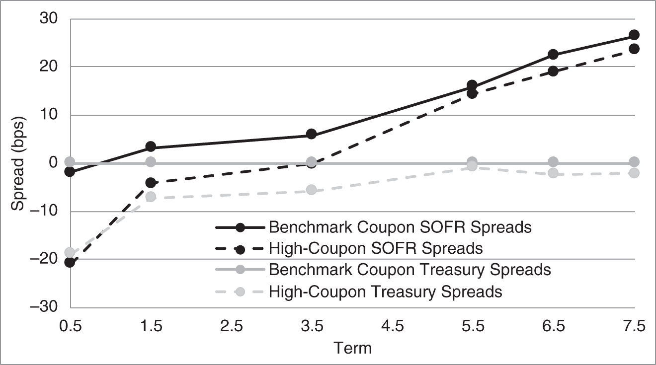
FIGURE 3.4 Spreads of Selected US Treasury Bonds to Benchmark Treasuries and to SOFR Swaps, as of May 14, 2021.
To understand this difference in relative valuations, Figure 3.5 graphs the two forward curves. Past a term of 2.5 years, the SOFR forward curve is not as steep as the Treasury forward curve. This means that the SOFR curve assigns relatively high prices to longer‐term Treasury bonds and, consequently, makes their market prices look relatively cheap. Equivalently, SOFR spreads at longer terms need to be larger to get pricing back up to the levels of Treasury forwards. The lesson here to practitioners is that using spreads against a curve from another market may have liquidity advantages, as mentioned earlier, but can complicate the interpretation of spreads and trades based on those spreads. In the present case, the relative cheapness of longer‐term, high‐coupon Treasuries, as indicated by their relatively large SOFR spreads, is actually a combination of their relative cheapness against the Treasury curve and the relative flatness of the SOFR curve. Furthermore, trades that attempt to lock in these spreads of Treasury bonds against SOFR spreads, called asset swaps, require trades not only in Treasuries but in matched‐maturity SOFR swaps as well. Chapter 14 discusses asset swap trades in greater detail.

FIGURE 3.5 Benchmark Treasury and SOFR Forward Rate Curves, as of May 14, 2021.
3.7 UNCHANGED RATE SCENARIOS FOR P&L ATTRIBUTION
This section and the next describe how ex‐post P&L or returns can be broken down into components so as to understand the sources of profits or losses from a trade or investment. One of these components, carry–roll‐down, is the change in value or the return of a bond or portfolio of bonds over time, assuming that “rates do not change” over the P&L or return horizon. The purpose of this section is to present two commonly assumed scenarios to represent rates not changing: realized forwards and an unchanged term structure.
TABLE 3.4 Realized Term Structure of Treasury Forward Rates on Various Dates, as of November 13, 2020. Rates Are in Percent.
| Term | 11/13/20 | 05/14/21 | 11/15/21 | 05/14/22 |
|---|---|---|---|---|
| 0.5 | 0.1013 | 0.1746 | 0.2429 | 0.2185 |
| 1.0 | 0.1746 | 0.2429 | 0.2185 | |
| 1.5 | 0.2429 | 0.2185 | ||
| 2.0 | 0.2185 |
Table 3.4 illustrates realized forward scenarios as of November 13, 2020, with sequential six‐month horizons. The 11/13/2020 column gives the then‐prevailing US Treasury term structure of six‐month forward rates. Using the notation of Chapter 2, the first six‐month forward rate, ![]() , is 0.1013%; the six‐month rate, six months forward,
, is 0.1013%; the six‐month rate, six months forward, ![]() , is 0.1746%; the six‐month rate, one year forward,
, is 0.1746%; the six‐month rate, one year forward, ![]() , is 0.2429%; etc. The next three columns give the assumed term structures of forward rates on subsequent dates. Note that the 11/13/2020 date is selected as a business day approximately six months before 05/14/2021, which is the pricing date for many of the examples in this text. The 11/15/2021 and 05/14/2022 dates are somewhat arbitrarily chosen as business days approximately six months apart.
, is 0.2429%; etc. The next three columns give the assumed term structures of forward rates on subsequent dates. Note that the 11/13/2020 date is selected as a business day approximately six months before 05/14/2021, which is the pricing date for many of the examples in this text. The 11/15/2021 and 05/14/2022 dates are somewhat arbitrarily chosen as business days approximately six months apart.
Realized forward scenarios assume that today's six‐month rate, ![]() years forward, will be the six‐month rate
years forward, will be the six‐month rate ![]() years from now. In terms of the table, the November 13, 2020, six‐month rate, six months forward, 0.1746%, is assumed to be the six‐month rate in six months, that is, on May 14, 2021. The November 13, 2020, six‐month rate, one year forward, 0.2429%, is assumed to be the six‐month rate on November 15, 2021; and the November 13, 2020, six‐month rate, 1.5 years forward, 0.2185%, is assumed to be the six‐month rate on May 14, 2022. Furthermore, all along the way, the forward rates slide down the curve. The November 13, 2020, six‐month rate, one‐year forward, 0.2429%, becomes the six‐month rate, six months forward, on May 14, 2021, before becoming the six‐month rate on November 15, 2021. And the November 13, 2020, six‐month rate, 1.5 years forward, 0.2185%, becomes the six‐month rate, one year forward, on May 14, 2021, and the six‐month rate, six months forward, on November 15, 2021, before becoming the six‐month rate on May 14, 2022.
years from now. In terms of the table, the November 13, 2020, six‐month rate, six months forward, 0.1746%, is assumed to be the six‐month rate in six months, that is, on May 14, 2021. The November 13, 2020, six‐month rate, one year forward, 0.2429%, is assumed to be the six‐month rate on November 15, 2021; and the November 13, 2020, six‐month rate, 1.5 years forward, 0.2185%, is assumed to be the six‐month rate on May 14, 2022. Furthermore, all along the way, the forward rates slide down the curve. The November 13, 2020, six‐month rate, one‐year forward, 0.2429%, becomes the six‐month rate, six months forward, on May 14, 2021, before becoming the six‐month rate on November 15, 2021. And the November 13, 2020, six‐month rate, 1.5 years forward, 0.2185%, becomes the six‐month rate, one year forward, on May 14, 2021, and the six‐month rate, six months forward, on November 15, 2021, before becoming the six‐month rate on May 14, 2022.
The scenario of an unchanged term structure assumes that all forward rates remain the same period after period. In terms of Table 3.4, this scenario assumes that the term structure of forward rates on November 13, 2020, is the same as the term structure on May 14, 2021, November 15, 2021, and May 14, 2022. In terms of rates, ![]() stays at 0.1013%;
stays at 0.1013%; ![]() stays at 0.1746%; and so forth.
stays at 0.1746%; and so forth.
TABLE 3.5 Return on a ![]() ‐Year Zero Coupon Bond Under the Scenarios of Realized Forward Rates and an Unchanged Term Structure, with Annual Periods.
‐Year Zero Coupon Bond Under the Scenarios of Realized Forward Rates and an Unchanged Term Structure, with Annual Periods.
| Realized Forwards | Unchanged Term Structure | |
|---|---|---|
Chapter 8 characterizes the realized forward scenario as the pure expectations hypothesis and the unchanged term structure scenarios as the pure risk premium hypothesis. For now, however, Table 3.5 gives some insight into bond returns under the two scenarios by deriving the annual return on a zero coupon bond of maturity ![]() , with annual periods. The price of the bonds today,
, with annual periods. The price of the bonds today, ![]() , are both given by discounting their maturing face value of one unit of currency by the annual forward rates
, are both given by discounting their maturing face value of one unit of currency by the annual forward rates ![]() through
through ![]() . In one year, the bonds are both
. In one year, the bonds are both ![]() ‐year zeros, and their prices,
‐year zeros, and their prices, ![]() , differ according to the assumed scenario. Under realized forwards, the first forward rate becomes
, differ according to the assumed scenario. Under realized forwards, the first forward rate becomes ![]() , etc., out to
, etc., out to ![]() , giving the
, giving the ![]() value in that column of the table. Under an unchanged term structure, the appropriate forward rates are
value in that column of the table. Under an unchanged term structure, the appropriate forward rates are ![]() through
through ![]() :
: ![]() drops out, because the bond matures in
drops out, because the bond matures in ![]() years. The last row of the table gives the one‐year return of the bond, which is simply
years. The last row of the table gives the one‐year return of the bond, which is simply ![]() , or
, or ![]() .
.
The table shows that, under realized forwards, the one‐year return on the ![]() ‐year zero is the one‐year rate,
‐year zero is the one‐year rate, ![]() . Appendix A3.3 shows that this result is very general: under realized forwards, the return on any bond equals the short‐term rate. And if the bond trades at a constant spread to the benchmark curve, the return equals the short‐term rate plus that spread. To the extent the scenario is considered reasonable, this result is useful for P&L attribution, because any return different from the short‐term rate is attributable not to the passage of time, but to other factors, like changes in rates or spreads.
. Appendix A3.3 shows that this result is very general: under realized forwards, the return on any bond equals the short‐term rate. And if the bond trades at a constant spread to the benchmark curve, the return equals the short‐term rate plus that spread. To the extent the scenario is considered reasonable, this result is useful for P&L attribution, because any return different from the short‐term rate is attributable not to the passage of time, but to other factors, like changes in rates or spreads.
Under the assumption of an unchanged term structure, the one‐year return on the ![]() ‐year zero is the initial forward rate from
‐year zero is the initial forward rate from ![]() to
to ![]() . This result does not generalize as easily as the return under realized forwards, and the intuition behind both results becomes clear in Chapter 8. For the purpose of this section, however, suffice it to say that if a trader or investment manager finds the unchanged term structure scenario a more reasonable expression of “rates stay the same,” then returns under that scenario can be considered a baseline, and return deviations from that baseline are attributed to other factors.
. This result does not generalize as easily as the return under realized forwards, and the intuition behind both results becomes clear in Chapter 8. For the purpose of this section, however, suffice it to say that if a trader or investment manager finds the unchanged term structure scenario a more reasonable expression of “rates stay the same,” then returns under that scenario can be considered a baseline, and return deviations from that baseline are attributed to other factors.
3.8 P&L ATTRIBUTION
As mentioned earlier, breaking down P&L or return into component parts is extremely useful for understanding how money is being made or lost in a trading book or investment portfolio. In addition, attribution reports can often catch errors of many sorts (e.g., buying or selling the wrong bond; buying instead of selling or vice versa; incorrect market or position data feeds).
P&L attribution can be quite detailed, but, for the purposes of this chapter, the focus is on a single bond rather than a portfolio; the holding period is fixed at a coupon payment period; and attribution is to four factors: cash carry, carry–roll‐down, changes in rates, and changes in spreads.6
Cash carry captures interim cash flows from a bond investment, typically from coupons and from financing arrangements (i.e., borrowing funds to buy bonds or borrowing bonds to short them). The example of this section ignores financing, however, which is the subject of Chapter 10.
Carry–roll‐down captures the P&L or return from changes in price when neither rates nor spreads change. The previous section described how rates not changing might be modeled as realized forwards or as an unchanged term structure. The example of this section assumes realized forwards.
Because “carry” and “roll‐down” are used differently by different practitioners, the nomenclature adopted here requires some elaboration. Broadly speaking, carry is meant to convey how much a position earns due to the passage of time, holding everything else constant. A clean example is a par bond when the term structure of interest rates is flat and unchanging. In that case, because the bond's price is always par, its carry is clearly its coupon income minus costs of financing. Another clean example is a premium bond when the term structure, again, is flat and unchanging. In that case, because the bond's price is pulled to par over time (Figure 3.1), its carry is clearly its coupon income minus the decline in price minus costs of financing.
Roll‐down, broadly speaking, is meant to convey how much a position earns as it matures and is valued at a different part of the term structure, holding everything else constant. A clean example of this concept is a forward loan. Referring to the rates in Table 3.4, say that, on November 13, 2020, an investor makes a six‐month loan, one year forward, at 0.2429%, and has adopted the unchanged term structure scenario for P&L attribution. Six months later, the investor's position will have matured to a six‐month loan, six months forward to be valued at the “unchanged” rate of 0.1746%, which is the six‐month rate, six months forward, on November 13, 2020. Hence, holding everything else constant, the forward loan has gained in value: the investor had locked in a loan rate of 0.2429% on November 13, 2020, and, six months later, the loan is valued at 0.1746%. In other words, the loan increased in value because it rolled down the curve.
While there are some cases in which it is clear how to separate carry from roll‐down, there are many cases in which it is not so clear. Consider a premium bond when the term structure is upward sloping and unchanging. The resulting P&L would be a combination of carry – coupon, pull‐to‐par, and financing costs – and roll‐down, as the bond's cash flows are discounted at lower rates.
This text takes the position that the important division in P&L attribution is between what happens due solely to the passage of time and what happens when rates and spreads change. Furthermore, to be consistent with the nomenclature in forwards and futures markets, discussed in Chapter 11, the phrase cash carry is preserved to mean coupon income minus financing costs. Therefore, carry–roll‐down here denotes P&L or return due to the passage of time excluding cash carry. The name reflects carry–roll‐down's being a mix of what might otherwise be classified as either carry or roll‐down.
The remaining two components of P&L or return described in this chapter, those due to changes in rates and to changes in spreads, are relatively self‐explanatory and are discussed presently.
The text now turns to a detailed P&L attribution for the US Treasury 7.625s of 11/15/2022 over the period November 13, 2020, to May 14, 2021. Note that both of these pricing dates are Fridays, so that settlement is on November 16, 2020, and May 17, 2021, respectively. Therefore, full prices given here include one and two days of accrued interest, respectively, and an investor over this holding period does not receive the coupon paid on November 15, 2020, but does receive the coupon paid on May 15, 2021.
The computation and results of the P&L attribution are given in Tables 3.6, 3.7, and 3.8. The first row of Table 3.6 gives the market price and spread of the 7.625s of 11/15/2022 as of the beginning of the period, November 13, 2020. This spread of ![]() 1.16 basis points is relative to the benchmark Treasury term structure on November 13, 2020, which is reported in the second column of Table 3.7. The computation of spread from market price is not shown here but can be computed along the same lines as Equation (3.14).
1.16 basis points is relative to the benchmark Treasury term structure on November 13, 2020, which is reported in the second column of Table 3.7. The computation of spread from market price is not shown here but can be computed along the same lines as Equation (3.14).
The second row of Table 3.6 computes a price for the bond as of the end of the period, May 14, 2021, assuming realized forwards – given in the third column of Table 3.7 – and an unchanged spread of ![]() 1.16 basis points. Once again, this spread calculation can be done along the lines of Equation (3.14). The change in price from 114.88, in the first row of Table 3.6, to 111.12, in the second row of the table, represents what happens to the bond price due to the passage of time alone: the realized forwards scenario is taken here to mean no change in rates, and the spread is also unchanged. Therefore, the dollar difference in these prices,
1.16 basis points. Once again, this spread calculation can be done along the lines of Equation (3.14). The change in price from 114.88, in the first row of Table 3.6, to 111.12, in the second row of the table, represents what happens to the bond price due to the passage of time alone: the realized forwards scenario is taken here to mean no change in rates, and the spread is also unchanged. Therefore, the dollar difference in these prices, ![]() 3.76, and the difference as a percentage of the initial price,
3.76, and the difference as a percentage of the initial price, ![]() 3.27%, is attributed to carry–roll‐down and reported as such in Table 3.8. The carry–roll‐down is large and negative because the bond has a coupon rate very much above the market rate and, consistent with the discussion in Section 3.2, its price is pulled down to par over time.
3.27%, is attributed to carry–roll‐down and reported as such in Table 3.8. The carry–roll‐down is large and negative because the bond has a coupon rate very much above the market rate and, consistent with the discussion in Section 3.2, its price is pulled down to par over time.
TABLE 3.6 Data for the P&L Attribution of the 7.625s of 11/15/2022 from November 13, 2020, to May 14, 2021. Spreads Are in Basis Points, and Percent Change Is Relative to Price on November 13, 2020.
| Pricing | Term | Percent | |||
|---|---|---|---|---|---|
| Date | Structure | Spread | Price | Change | Change |
| 11/13/2020 | 11/13/2020 | 114.87654 | |||
| 5/14/2021 | Realized Forwards | 111.11555 | |||
| 5/14/2021 | 5/14/2021 | 111.29847 | 0.18292 | 0.1592% | |
| 5/14/2021 | 5/14/2021 | 111.39690 | 0.09843 | 0.0857% |
TABLE 3.7 Term Structures of Forward Rates for the P&L Attribution of the 7.625s of 11/15/2022 from November 13, 2020, to May 14, 2021. Rates Are in Percent.
| Term Structures of Forward Rates | |||
|---|---|---|---|
| Term | 11/14/20 | Realized Forwards | 5/14/21 |
| 0.5 | 0.1013 | 0.1746 | 0.0154 |
| 1.0 | 0.1746 | 0.2429 | 0.1008 |
| 1.5 | 0.2429 | 0.2185 | 0.1833 |
| 2.0 | 0.2185 | ||
The third row of Table 3.6 computes a price for the bond as of May 14, 2021, assuming the actual Treasury term structure on that date, given in the fourth column of Table 3.7, and a still‐unchanged spread from the beginning of the period. Yet again, this price can be computed along the lines of Equation (3.14). The difference between the resulting price of 111.30 and the price of 111.12 in the second row represents the P&L due to a change in rates – from the realized forwards scenario of “no change” to the actual term structure on May 14, 2021. The differences of 0.18 and 0.16% are reported in Table 3.8 as the rates component row of the attribution. This component of the attribution is positive because, as is clear from Table 3.7, rates fell from the realized forwards scenario to the actual rates on May 14, 2021.
TABLE 3.8 P&L Attribution of the 7.625s of 11/15/2022 from November 13, 2020, to May 14, 2021. Returns Are in Percent.
| Component | P&L | Return |
|---|---|---|
| Cash Carry | 3.81250 | 3.3188 |
| Carry–Roll‐Down | ||
| Rates | 0.18292 | 0.1592 |
| Spread | 0.09843 | 0.0857 |
| Total | 0.33286 | 0.2898 |
The fourth and final row of Table 3.6 gives the market price of the bond on May 14, 2021, along with its ![]() 7.27 basis‐point spread relative to the benchmark Treasury term structure on that date. This spread is actually computed in Equation (3.14). The difference between the May 14, 2021, market price and the price in the third row of the table represents the spread component of the attribution, as the only change from the third to the fourth rows is the spread. The differences of 0.10 and 0.09% are reported as such in Table 3.8. This component is positive because the bond's spread fell from November 13, 2020, to May 14, 2021; that is, the bond became richer relative to the benchmark Treasury curve.
7.27 basis‐point spread relative to the benchmark Treasury term structure on that date. This spread is actually computed in Equation (3.14). The difference between the May 14, 2021, market price and the price in the third row of the table represents the spread component of the attribution, as the only change from the third to the fourth rows is the spread. The differences of 0.10 and 0.09% are reported as such in Table 3.8. This component is positive because the bond's spread fell from November 13, 2020, to May 14, 2021; that is, the bond became richer relative to the benchmark Treasury curve.
Table 3.8 summarizes the P&L and return attribution of the 7.625s of 11/15/2022 over the six‐month period from November 13, 2020, to May 14, 2021. The first row, which has not yet been discussed, is the cash carry of 3.8125, that is, the coupon payment on May 15, 2021. (Recall that because the pricing date is on May 14 and the settlement date on May 17, the investor receives the May 15 coupon payment.) As a whole, the table breaks down the total dollar P&L of 0.33 and the total return 0.2898% into the component parts of cash carry, carry–roll‐down, rates, and spread. Note that the sum of the cash carry and carry–roll‐down return components equals 0.0449%, which is the six‐month rate plus the bond spread on May 14, 2021, all divided by two, that is ![]() . This is, of course, no coincidence. As highlighted in the previous section, the annual return of any bond under the realized forward scenario is the short‐term rate plus the spread, or half of that over a six‐month horizon.
. This is, of course, no coincidence. As highlighted in the previous section, the annual return of any bond under the realized forward scenario is the short‐term rate plus the spread, or half of that over a six‐month horizon.
A trader or investor can use P&L and return attribution in several ways. First, as mentioned earlier, any surprises here might be due to errors in building positions, booking positions, or data feeds. Second, because cash carry and carry–roll‐down can be computed at the beginning of the period, the trader or investor can decide whether the cash flow properties of the position are acceptable. More specifically, a trade or investment that is expected to do well in the long run but expected to bleed cash in the short run may or may not be acceptable in all institutional settings. In the present example, it is known at the beginning of the period that the “no change” case will result in a positive cash flow of ![]() or about 0.05 cents before financing costs. Once financing costs are considered, this central case might be negative and might, in that case, be unacceptable.
or about 0.05 cents before financing costs. Once financing costs are considered, this central case might be negative and might, in that case, be unacceptable.
A third use of P&L and return attribution is as an ex‐post check on performance. Did the investor or trader have an ex‐ante view on rates and, if so, how did realized rate changes compare with that view? Was there a view about how the spread of the bond would evolve and, again, if so, how did that view compare with the realized spread? Many traders and investors like to ask the following, when setting up a position: What could happen to this position that would convince me that I don't understand the relevant market forces? They would then promise themselves to exit the position if it turned out that their understanding was flawed. P&L and return attribution is a valuable tool in that discipline by revealing exactly where money is made or lost.
NOTES
- 1 For consistency with discussions later in the chapter, note that the two dates are actually November 13, 2020, and May 14, 2021. These two dates are Fridays, and the prices given here are full prices for settlement on November 16, 2020, and May 17, 2021, respectively, which means that the investor does not receive the coupon paid on November 15, 2020, but does receive the coupon paid on May 15, 2021.
- 2 This is only approximately correct because the settlement date is actually May 17, 2021. Hence, there is slightly less than one semiannual period to the first coupon payment date. Appendix A3.1 defines yield in this more general case.
- 3 There are no bonds with maturities between May 2031 and February 2036 because the Treasury stopped issuing new 30‐year bonds after May 2001 and started issuing them again in February 2006.
- 4 In the case of a bond with no embedded options, bond spreads are the same as option‐adjusted spreads, which are described in Chapter 7.
- 5 In some contexts, like the corporate bond market, practitioners often define a term structure of spreads; that is, unlike in Equation (3.14), they allow a different spread to be added to each forward rate. This could capture, for example, the long‐term bonds of a particular corporation selling at a higher spread to Treasury bonds than its short‐term bonds. The discussion continues here, however, with a single spread.
- 6 More detailed analyses, instead of considering rates changes as a single change from one term structure to the next, consider, for instance, changes to the level of rates and the steepness of the term structure separately, or consider changes to individual segments of the term structure separately. These choices can be understood more fully in the context of the multi‐factor risk metrics in Chapters 5 and 6. More detailed analyses can also include more spreads, for example, the spread of Treasury rates to repo or financing rates; the spread of swap rates to Treasury rates; and the spread of various corporate rates to swap rates.