
CHAPTER 14
Corporate Debt and Credit Default Swaps
Corporations borrow money to fund their operations, transactions (e.g., mergers and acquisitions), and changes to capital structure (e.g., refinance existing debt, stock repurchases). The loans and bonds used to raise these funds are subject to credit risk, because corporations may not make good on their promises to pay interest and repay principal. Lenders, in turn, require compensation for bearing credit risk in the form of higher returns. The cash flows of credit default swaps (CDS) also depend on the payment or nonpayment of debt obligations but are not themselves obligations of corporate issuers. In other words, through CDS contracts, market participants trade corporate credit risks with each other. While this chapter focuses mostly on corporate debt, much of the discussion applies to sovereign and municipal debt as well, because the debt obligations of many governments have at times been perceived as subject to nontrivial probabilities of default.
Many market participants rely to some extent on rating agencies to measure the credit risk of borrowers and their loans and bonds. The long‐term debt ratings classifications of the three major rating agencies in the United States are given in Table 14.1. More granular breakdowns of each of these broad ratings classifications are also available, and short‐term debt has its own, separate scales.1
TABLE 14.1 Long‐Term Debt Ratings Classifications. The Ratings in Each Entry Are Listed in Decreasing Order of Creditworthiness.
| Speculative Grade/ | |||
|---|---|---|---|
| Agency | Investment Grade | High Yield | Default |
| Moody's | Aaa, Aa, A, Baa | Ba, B, Caa, Ca | C |
| S&P, Fitch | AAA, AA, A, BBB | BB, B, CCC, CC, C | D |
14.1 CORPORATE BONDS AND LOANS
Large and highly creditworthy corporations in the United States tend to borrow money for fixed terms in public markets through commercial paper (CP), medium‐term notes (MTNs), and corporate bonds. CP is typically a discount (i.e., zero coupon) instrument that is either unsecured, backed by a letter of credit from a bank, or secured by assets. CP is exempt from Securities and Exchange Commission (SEC) registration, along with its associated costs, so long as the paper matures in less than 270 days and its proceeds are used for short‐term purposes (rather than, for example, building a factory). With its high credit quality and short‐term maturity, CP is a particularly inexpensive and liquid way for the most creditworthy corporations to raise short‐term funds. CP borrowing does, however, expose a corporation to the funding or liquidity risk of having to roll outstanding CP as it matures into new CP issues.
Corporations sell MTNs in public markets to raise money with customized payment terms. Historically, MTNs primarily filled the maturity gap between CP and longer‐term bonds but are now better characterized as debt instruments customized to suit the needs of individual issuers and investors. MTNs first became popular in the United States in the early 1980s, with the introduction of SEC shelf registrations. These programs allow issuers to register once to sell notes opportunistically, over time, at terms that can be adjusted at the time of each sale.
For longer‐term borrowing in public markets with relatively standard payment terms, corporations sell bonds, which, in the United States, have to be registered with the SEC. Corporate bonds are typically coupon‐bearing, fixed‐rate securities, but there is a much smaller market for floating‐rate notes (FRNs). The interest rate on FRNs is typically set equal to a short‐term reference rate plus a fixed spread, although a reference rate might be multiplied by a factor or leverage, and the spread might vary over time with the credit rating of the issuer. The short‐term reference rate for FRNs had traditionally been the London Interbank Offered Rate (LIBOR) but is now transitioning to the Secured Overnight Financing Rate (SOFR) and other non‐LIBOR alternatives (Chapters 12 and 13).
Smaller and less creditworthy corporations, which cannot typically raise funds in public markets, tend to borrow money through private placements of bonds and through bank loans. In a privately placed bond issue, the borrower tailors terms to satisfy its own requirements and those of a relatively small group of lenders. Insurance companies are the most significant investors in this market, though other asset managers participate as well. Privately placed bonds are exempt from SEC registration precisely because they may be sold only to investors deemed “sophisticated.”
Bank loans tend to be floating‐rate instruments, although borrowers sometimes convert their debt into a fixed rate by paying fixed to and receiving floating from a bank in an accompanying interest rate swap, which the bank, in turn, hedges with a dealer (Chapter 13). From the bank perspective, floating‐rate loans have the advantage of matching floating‐rate liabilities, which are mostly deposits, but also include wholesale funding like commercial paper. Also, floating‐rate loans are the easiest to sell in the secondary market for bank loans.
Traditionally, banks made loans and held them to term. And if a single borrower needed a loan that was too large for one bank, either because funds were not readily available or, more likely, because the resulting credit risk would be too significant for one bank, several banks would form a group or syndicate in which each would make and hold a smaller loan to that large borrower. The last few decades, however, have seen phenomenal growth in the secondary market for loans, which allows banks to sell loans they have made to institutional investors. In this way, banks can earn fees on making, servicing, and monitoring loans without having to warehouse all of the associated credit risk. At present, in fact, the overwhelming majority of relatively low‐quality or leveraged loans are held not by banks, but by institutional investors. While some leveraged loans are bought from banks directly by insurance companies, mutual funds, and hedge funds, much of the growth of the secondary market for bank loans has been through the indirect sale of loans to institutional investors through collateralized loan obligations (CLOs).
Collateralized Loan Obligations
A CLO is a vehicle that purchases a portfolio of leveraged loans financed by the sale of several debt classes or tranches and equity or subordinated notes. Table 14.2 lists the debt tranches of a particular CLO issued in May 2019. Essentially, interest and principal payments from the underlying portfolio of leveraged loans flow to the tranches from the top down, while any credit losses are allocated from the bottom up.2 Senior Secured Floating‐Rate Note Classes X, A‐1, A‐2, and B are paid interest and principal from the underlying loans, while Mezzanine Secured Deferrable classes C, D, and E are paid to the extent that additional cash flows from the underlying loans are available. Any credit losses from the underlying loans are first applied to the equity or Subordinated Notes, then to the Mezzanine tranches, and only then, if necessary, to the Senior Secured tranches. Furthermore, CLO debt tranches are protected by constraints imposed on the creditworthiness of the underlying loans and on the concentration of loans to a particular borrower or industry, along with various ongoing tests as to the sufficiency of interest and collateral. In short, this CLO, from an underlying portfolio of $634,125,000 leveraged loans, created $414,225,000 of X, A‐1, and A‐2 tranches with AAA or Aaa ratings; an additional $64,600,000 B tranches with an AA rating; and so forth.
TABLE 14.2 Tranches of Apidos CLO XXXI, May 2019. All Tranches Mature in April 2031.
| Amount | Rating | Spread over | ||
|---|---|---|---|---|
| Class | Description | ($millions) | S&P/Moody's | LIBOR (bps) |
| X | Sr. Secured FRNs | 4.725 | AAA/– | 65 |
| A‐1 | Sr. Secured FRNs | 370.150 | AAA/Aaa | 133 |
| A‐2 | Sr. Secured FRNs | 39.350 | –/Aaa | 165 |
| B | Sr. Secured FRNs | 64.600 | AA/– | 190 |
| C | Mezzanine Secured Deferrable FRNs | 40.300 | A/– | 255 |
| D | Mezzanine Secured Deferrable FRNs | 36.200 | BBB–/– | 365 |
| E | Mezzanine Secured Deferrable FRNs | 27.400 | –/Ba3 | 675 |
| – | Subordinated Notes | 51.400 | – | – |
| Total | 634.125 | |||
Compensation for buying lower‐rated tranches comes in the form of earning a higher spread. As shown in the last column if Table 14.2, spreads range from 65 basis points for the AAA‐rated X Class to 675 basis points for the Ba3‐rated Class E tranche.3 The return on equity, of course, is determined by whatever is left over after paying all of the more senior claims.
The different credit risk profiles of the different tranches in a CLO tend to attract different groups of investors. Banks tend to hold or purchase the AAA/Aaa and AA/Aa tranches; insurance companies and pension funds invest in a range of tranches; and hedge funds and alternative asset managers buy the lower‐rate tranches. Outside investors and the CLO originators hold the equity.
By way of summarizing trends over the last few decades, the growth of the secondary market for leveraged loans, abetted by the CLO market, has blurred the distinction between leveraged loans and high‐yield bonds. Corporations have greater flexibility to borrow in one market or the other, and asset managers actively decide to invest in one market or the other, with all choices depending on individual preferences or requirements and on market conditions.
Seniority, Covenants, and Call Provisions
When selling a debt issue, a corporation enters into a contract with bondholders, called an indenture, which is enforced by a trustee. Aside from payment terms (e.g., interest, principal, and maturity), the indenture specifies the priority of the issue in the event of default. For example, one bond issue might be secured by a particular set of assets; a second might be unsecured, but “senior” to other issues; and a third might be “subordinated” to higher‐ranking issues. In this example, should a corporation be reorganized or liquidated through bankruptcy according to “strict priority,” proceeds from selling ring‐fenced assets would be applied first to satisfy the claims of the secured bondholders. Any remaining proceeds, together with other assets of the corporation, would be applied next to satisfy the claims of the senior bondholders. Finally, whatever value remains would be used to satisfy the claims of the subordinated bondholders. In practice, because reorganizations involve negotiation and include equity holders, strict priority may not always precisely predict the settlement of debt claims.
Indentures also include covenants to protect the claims of bondholders. Examples include maintaining various financial ratios; restricting the amount of cash that can be paid to stockholders; requiring a corporation to repurchase a debt issue after a change of control; limiting the total amount of new debt incurred by the corporation; and preventing the sale of debt with higher seniority than that of an outstanding debt issue.
As a final point of discussion, indentures often include call provisions or embedded call options, which allow a corporation to repurchase bonds from bondholders at some fixed schedule of prices. A simple example would be a 20‐year bond that the company can repurchase at par or face value anytime after 10 years. A more complex example would be a 4% 30‐year bond that the company can repurchase after 10 years at a price of 102 (100 plus half the coupon); at a price of 101.90 after 11 years; at a price of 101.80 after 12 years.
The original purpose of call provisions was to enable corporations to extinguish a bond issue – without having to track down and purchase every outstanding bond – perhaps to remove covenants that prohibited what had become value‐added activities, or perhaps to change the corporation's existing capital structure. As interest rates became more volatile in the early 1980s, these call provisions became valuable as interest rate options: the value of the right to purchase a bond at some fixed price increases as rates decline (bond prices increase) and also as rate volatility increases. At the same time, of course, corporations issuing debt with call provisions have to pay investors for that option through a higher coupon rate. Chapter 16 describes the pricing of these call provisions.
TABLE 14.3 Call Provision of the Hertz 6s of 01/15/2028. The Bond Was Issued in November 2019.
| Dates | Call Price |
|---|---|
| Before 01/15/2023 | Make‐Whole Price |
| Treasury 2.75s of 02/15/2028 +50bps | |
| 01/15/2023 to 01/14/2024 | 103.00 |
| 01/15/2024 to 01/14/2025 | 101.50 |
| On or after 01/15/2025 | 100.00 |
Since the mid‐1990s, however, the most common call provision has become the make‐whole call. For example, in a private placement in November 2019, Hertz sold the 6s of 01/15/2028, with the make‐whole call provision described in Table 14.3. Before January 15, 2023, Hertz can repurchase the bonds from investors at a yield 50 basis points above the yield of the US Treasury 2.75s of 02/15/2028. From January 15, 2023, on, the call is at the schedule of fixed prices shown in the table. The idea behind the make‐whole call is to give the issuer flexibility to manage its debt without its having to purchase an expensive interest rate option. Unlike the case of a call price that is fixed, when yields fall, the yield of the Treasury benchmark falls too, and the make‐whole call price increases. Hence, the interest rate option value of the make‐whole call is extremely limited. In fact, in theory, the make‐whole call has option value only if the market spread of the Hertz bonds over Treasuries falls: in that scenario, the value of the Hertz bond increases without a corresponding fall in the yield of the Treasury bond and a corresponding increase of the make‐whole price. In practice, however, the value of this spread option is mitigated by setting the make‐whole spread out‐of‐the‐money. For example, when Hertz issued the 6s of 01/15/2028 in November 2019, its spread over the Treasury benchmark was 423 basis points. This means that its bond spread would have to fall a very large ![]() or 373 basis points before the make‐whole provision was in‐the‐money as an option on spread. Overall, of course, the call provision of the Hertz 6s of 01/15/2028 derives option value from the schedule of fixed call prices from January 15, 2023.
or 373 basis points before the make‐whole provision was in‐the‐money as an option on spread. Overall, of course, the call provision of the Hertz 6s of 01/15/2028 derives option value from the schedule of fixed call prices from January 15, 2023.
14.2 DEFAULT RATES, RECOVERY RATES, AND CREDIT LOSSES
While investors in nearly risk‐free government bonds can focus exclusively on interest rate risk, investors in corporate securities have to focus on credit risk as well, often expressed in terms of default rates, recovery rates, and credit losses. After analysis, an investor might estimate that, over a five‐year horizon, a particular portfolio of bonds will experience a default rate of 10%, meaning that, for every $100 of face amount, $10 will default. Furthermore, the investor might estimate that the defaulting bonds in the portfolio will experience a recovery rate of 40% of face amount, or, equivalently, will suffer a loss equal to the remaining 60% of face amount. Putting these two estimates together, the investor expects, over a five‐year horizon, that credit losses on the portfolio will be ![]() .
.
Table 14.4 shows average historical values for these quantities, over the period 1983–2020, for senior unsecured bonds, by rating. The results are useful for appreciating the average magnitude of credit risk. For investment‐grade senior unsecured bonds, the average five‐year default rates and recovery rates are 0.9% and 44.5%, respectively, giving an average credit loss of 0.5%. For speculative‐grade senior unsecured bonds, the average default rate is much higher, at 19.6%, though the average recovery rate is only marginally lower, at 38.3%. Combining these two averages gives a much higher credit loss of 12.2%. The standard assumption in the industry that recovery rates are about 40% is justified by historical data like those presented in Table 14.4.4
While historical averages are useful in thinking about credit risk, credit conditions can vary dramatically over time. For example, extending the sample of Table 14.4 to include the years after the Great Depression raises the five‐year default rate on investment‐grade debt from 0.9% to 1.4%. And within the sample period of the table, Figure 14.1 shows the variability of credit losses for investment‐grade and high‐yield bonds. High‐yield losses were particularly high in the late 1980s, following the rapid growth in that market; in 2000–2002, which included the “dot‐com” crash and the failures of Enron and WorldCom; in the financial crisis of 2007–2009; in 2016, from stresses caused by low prices in energy markets; and, most recently, during the pandemic and economic shutdowns of 2020.
TABLE 14.4 Average Five‐Year Default Rates, Senior Unsecured Bond Recovery Rates, and Credit Losses, 1983–2020. All Entries Are in Percent.
| Default | Recovery | Credit | |
|---|---|---|---|
| Rating | Rate | Rate | Loss |
| Investment Grade | 0.9 | 44.5 | 0.5 |
| Speculative Grade | 19.6 | 38.3 | 12.2 |
| All | 7.4 | 38.9 | 4.6 |
Source: Moody's Investors Service

FIGURE 14.1 Credit Losses for Senior Unsecured Bonds, 1983–2020.
Source: Moody's Investors Service.
Table 14.4 and Figure 14.1 report credit losses for senior unsecured bonds. Investment outcomes vary significantly, however, across loans and bonds of different seniority. Over the same sample period as in the table and figure, Moody's reports that bond recovery rates were 22% for junior subordinated; 38% for senior unsecured; and 54% for first lien (i.e., the highest priority secured claim). For bank loans, average recovery rates were 46% for senior unsecured; 65% for first lien; and 32% for second lien.
A recent example of the impact of seniority, illustrated in Table 14.5, is the price behavior of Hertz bonds through its bankruptcy filing on May 22, 2020. Before the pandemic, as of February 21, 2020, when default was a remote contingency, the prices of Hertz' secured and unsecured bonds were above par, with the higher price of the unsecured reflecting its longer maturity at an above‐market coupon. By May 14, 2020, after the pandemic and shutdowns devastated the rental car business, the prices of Hertz bonds plummeted, with the price of the secured bond now significantly higher: with default imminent, the seniority of the secured bonds was much more important than the seemingly distant prospect of the unsecured bond's cash flows through 2028. Soon after, however, in the wake of the economy's rapid recovery, Hertz's bond prices recovered dramatically as well. There was still much uncertainty as to the bonds' creditworthiness, however. The June 15, 2020, prices in the table show that the secured bonds still sold at a significant premium to the unsecured. By way of epilogue, Hertz emerged from bankruptcy at the end of June 2021, and its bonds recovered their full principal value.
TABLE 14.5 Hertz Corporation, Selected Bond Prices on Three Dates in 2020.
| Priority | Coupon | Maturity | Feb 21 | May 14 | Jun 15 |
|---|---|---|---|---|---|
| Sr. Secured 2nd Lien | 7.625 | 06/01/2022 | 103.10 | 19.97 | 77.00 |
| Sr. Unsecured | 6.000 | 01/15/2028 | 104.29 | 11.25 | 43.50 |
Potential credit losses are directly relevant for investors expecting to hold bonds to maturity. Investors with shorter horizons, however, are also concerned about credit deterioration, which causes bond prices to fall before a realized default and credit loss. One manifestation of credit changes are rating transitions, in which a rating agency upgrades or downgrades a rating. Table 14.6 gives average historical one‐year transition rates, or, more specifically, the rates at which bonds starting at a particular rating, over the following year, are upgraded, experience no change, are downgraded (including defaults), or become unrated. Becoming unrated may be a negative credit event but could also indicate a credit‐neutral event like an acquisition. In any case, the table shows that downgrades over a one‐year horizon are not uncommon, averaging from about 4% to 10% for bonds rated B or above, and over 28% for CCC/C‐rated bonds. Upgrades occur as well, but with less frequency. Though not shown in the table, upgrades and downgrades vary with the business cycle, like the credit losses in Figure 14.1.
TABLE 14.6 Average One‐Year Transition Rates, 1981–2020. All Entries Are in Percent.
| Rating | Upgrade | No Change | Downgrade | No Rating |
|---|---|---|---|---|
| AAA | 0.0 | 87.1 | 9.8 | 3.1 |
| AA | 0.5 | 87.2 | 8.4 | 3.9 |
| A | 1.6 | 88.6 | 5.4 | 4.4 |
| BBB | 3.3 | 86.5 | 4.3 | 5.9 |
| BB | 4.7 | 77.8 | 8.0 | 9.5 |
| B | 4.8 | 74.6 | 8.3 | 12.3 |
| CCC/C | 13.3 | 43.1 | 28.3 | 15.3 |
Source: S&P Global Ratings; and Author Calculations
14.3 CREDIT SPREADS
Credit spreads are the differences between the relatively high rates earned on fixed income instruments that are subject to credit risk and the relatively low rates on instruments with little or no credit risk. The simplest measure of credit spread is the yield spread, which is the difference between the yield on a bond and the rate or yield on a similar maturity interest rate swap or highly creditworthy government bond. Yield spreads, however, suffer from a number of drawbacks. First, a sufficiently liquid government bond or swap with a similar maturity might not exist. Second, yields reflect not only credit risk, but also the structure of a bond's cash flows. (See the discussion of the “coupon effect” in Chapter 3.) Third, yields reflect the value of embedded options, like the fixed‐price call provisions discussed earlier, which have nothing to do with credit risk.
A better measure of credit spread is referred to in this chapter as the bond spread. This term includes the spread defined in Chapter 3 and the more general option‐adjusted spread (OAS) defined in Chapter 7. In the credit context, a bond spread is computed by assuming no default and finding the spread over a benchmark curve that prices a bond as it is priced in the market. Because the market price incorporates the risk of default while this pricing methodology does not, the bond spread is a metric of credit risk. Unlike yield spreads, bond spreads properly account for maturity and the structure of cash flows. This approach, therefore, is suitable for bonds without embedded options. For bonds with embedded options, OAS is more appropriate: by design, its computation of price accounts for the value of embedded options and, therefore, any remaining spread to the benchmark curve can be reasonably attributed to credit risk. Furthermore, as explained in Chapters 3 and 7, the bond spread and OAS can be interpreted as the extra spread earned by a bond if interest rates are unchanged or hedged against; if the spread is unchanged; and if the bond does not default.
The measures of credit spread in this section are illustrated with the Genworth 4.90s of 08/15/2023, a speculative‐grade bond issued by an insurance company. Table 14.7 gives various measures of credit spread for this bond, as of August 15, 2021, when the 4.90s of 08/15/2023 have exactly two years to maturity. Given the market yield of 5.596% and the two‐year LIBOR swap rate of 0.288%, the yield spread is the difference between those two rates, or 530.8 basis points. The bond spread, given the bond's market price of 98.70 and the term structure of forward swap rates as of the pricing date, is 531.1 basis points.5 Then, in the sense of the previous paragraph, the Genworth bond earns an annual rate of LIBOR plus 531.1 basis points.
TABLE 14.7 Selected Credit Spreads for the Genworth 4.90s of 08/15/2023, as of August 15, 2021. The Price of the Bond is 98.70; Its Yield is 5.596%; and the Par Swap Rate Is 0.288%. Spreads Are in Basis Points.
| Spread Type | Spread |
|---|---|
| Yield Spread | 530.8 |
| Bond Spread | 531.1 |
| Par‐Par Asset Swap Spread | 526.4 |
| Market Value Asset Swap Spread | 533.3 |
Other popular measures of spread are asset swap spreads. The point of an asset swap is to transform a fixed‐rate, coupon bond into an asset that earns a spread over a short‐term rate, like LIBOR. In the context of this chapter, asset swaps enable investors to earn credit spreads without having to bear the interest rate risk of long‐term, fixed‐rate bonds.
Figure 14.2 illustrates one type of asset swap, the par‐par asset swap, or, more simply, the par asset swap. Thin lines indicate cash flows at the initiation of the asset swap; heavy lines indicate intermediate cash flows; and dashed lines indicate cash flows at the maturity of the swap. At initiation, the asset swapper buys the bond for ![]() per 100 face amount, earning a periodic coupon payment of
per 100 face amount, earning a periodic coupon payment of ![]() . The purchase price is financed with 100 from the repo desk and
. The purchase price is financed with 100 from the repo desk and ![]() from the swap desk.6 Finally, through an interest rate swap to the maturity of the bond, in addition to the up‐front payment just mentioned, the asset swapper periodically pays
from the swap desk.6 Finally, through an interest rate swap to the maturity of the bond, in addition to the up‐front payment just mentioned, the asset swapper periodically pays ![]() in exchange for receiving LIBOR plus the spread,
in exchange for receiving LIBOR plus the spread, ![]() , on 100. Note that this trade requires no cash at initiation; earns LIBOR plus
, on 100. Note that this trade requires no cash at initiation; earns LIBOR plus ![]() minus the repo rate over the life of the bond, so long as the bond does not default; and requires no cash at maturity, again, so long as the bond does not default. Hence, as desired, the investor has converted the fixed coupon payments of a bond into floating payments of LIBOR plus
minus the repo rate over the life of the bond, so long as the bond does not default; and requires no cash at maturity, again, so long as the bond does not default. Hence, as desired, the investor has converted the fixed coupon payments of a bond into floating payments of LIBOR plus ![]() . Of course, there are losses if the bond defaults: in that case, the asset swapper has to make coupon payments to the swap desk and, at maturity, pay 100 to the repo desk, even though these payments will not be fully realized from the defaulted bond.
. Of course, there are losses if the bond defaults: in that case, the asset swapper has to make coupon payments to the swap desk and, at maturity, pay 100 to the repo desk, even though these payments will not be fully realized from the defaulted bond.
The par asset swap spread, ![]() , can be determined by the condition that the interest rate swap with the swap desk is fair, that is, that the initial payment plus the present value of the floating leg equals the present value of the fixed leg, where discounting is at market swap rates.7 Mathematically, let
, can be determined by the condition that the interest rate swap with the swap desk is fair, that is, that the initial payment plus the present value of the floating leg equals the present value of the fixed leg, where discounting is at market swap rates.7 Mathematically, let ![]() and
and ![]() be the factors such that
be the factors such that ![]() gives the present value of the payments of
gives the present value of the payments of ![]() on the fixed side of the swap and such that
on the fixed side of the swap and such that ![]() gives the present value of the payments of
gives the present value of the payments of ![]() on the floating side.8 Let
on the floating side.8 Let ![]() be the discount factor for cash flows at maturity. Also, along the lines of Chapter 13, include a fictional notional amount of 100 at maturity on both legs of the swap, and note that the present value of receiving LIBOR and the final notional amount is par. Then, the fair pricing condition for the swap is,
be the discount factor for cash flows at maturity. Also, along the lines of Chapter 13, include a fictional notional amount of 100 at maturity on both legs of the swap, and note that the present value of receiving LIBOR and the final notional amount is par. Then, the fair pricing condition for the swap is,

FIGURE 14.2 A Par‐Par Asset Swap with Financing.
From Equation (14.1), for a given swap rate curve, as the credit risk of the bond increases, ![]() decreases, which, in turn, increases the asset swap spread,
decreases, which, in turn, increases the asset swap spread, ![]() . Table 14.7 reports that, as of August 15, 2021, the par asset swap spread of the Genworth 4.90s of 08/15/2023 is 526.4 basis points.
. Table 14.7 reports that, as of August 15, 2021, the par asset swap spread of the Genworth 4.90s of 08/15/2023 is 526.4 basis points.
A second flavor of asset swaps, namely, a market value asset swap, is illustrated in Figure 14.3. The market value asset swap differs from the par asset swap in that ![]() is borrowed from the repo desk, rather than 100;
is borrowed from the repo desk, rather than 100; ![]() is paid by the swap desk at the maturity rather than the initiation of the swap; and, as a result, LIBOR plus the spread,
is paid by the swap desk at the maturity rather than the initiation of the swap; and, as a result, LIBOR plus the spread, ![]() , is earned on
, is earned on ![]() rather than 100. Following the same notation and logic as in the case of the par asset swap, the fair market value asset swap spread is given by,
rather than 100. Following the same notation and logic as in the case of the par asset swap, the fair market value asset swap spread is given by,
where the final equality uses Equation (14.1). According to Table 14.7, the market value asset swap spread of the Genworth 4.90s of 08/15/2023, as of August 15, 2021, is 533.3 basis points. The relationship between the two asset swap spreads is quite intuitive: an investor can earn ![]() on 100 or
on 100 or ![]() on
on ![]() , which, from Equation (14.2), gives the same result. The choice between the two asset swap trades, therefore, depends not on earnings, but on collateral and counterparty risk considerations.9
, which, from Equation (14.2), gives the same result. The choice between the two asset swap trades, therefore, depends not on earnings, but on collateral and counterparty risk considerations.9

FIGURE 14.3 A Market Value Asset Swap with Financing.
The final measure of credit spread considered in this section is an effective spread for corporate FRNs no longer priced at par. When an FRN is priced at par, its spread is particularly easy to interpret as a spread over the short‐term rate benchmark received in exchange for bearing credit risk. Over time, however, as the credit quality of the issuer changes, the price of an FRN with a fixed spread changes. As a result, because an investor pays a premium or gets a discount to face amount when buying the FRN, in addition to its spread, that spread is no longer as easily interpreted.
The effective spread converts an FRN's premium or discount into a run rate and adds it to the actual spread. Let the actual spread be ![]() ; the price of the floater
; the price of the floater ![]() ; the present value factor, as before
; the present value factor, as before ![]() ; and the effective spread
; and the effective spread ![]() . Then, investors are indifferent between receiving
. Then, investors are indifferent between receiving ![]() for a price of
for a price of ![]() and
and ![]() for a price of 100 if,
for a price of 100 if,
This section concludes by noting that the trades described here for earning the credit spread are subject not only to the risk of default, but also to financing risk. Whenever a bond is purchased for a relatively long‐term holding period, but is financed with short‐term repo, there is the risk that the repo rate will increase by more than the discounting or benchmark rates. In that case, the bond will earn less than the benchmark short‐term rate (e.g., LIBOR) plus the spread. An even more extreme risk is that repo lenders will refuse to roll positions, because they no longer wish to lend to the borrower, because they no longer wish to lend against a particular bond, or because they need the cash themselves. In that scenario, corporate bond investors with short‐term repo financing will have to sell their bonds, most likely at a loss, to repay outstanding repo loans. Financing risk in the context of credit risk appears again, later in this chapter, as a key difference between bonds and credit default swaps.
14.4 CREDIT RISK PREMIUM
If credit spreads, on average, just compensated for credit losses, then risk‐averse investors would just as soon buy safe government bonds at the same average return, but without the downside risk. For corporate debt to be attractive, therefore, spreads must not only compensate for credit losses, but also provide an additional credit risk premium. This section reviews some evidence that, on average, corporate bond spreads do, indeed, more than compensate for credit losses.
One study estimates that the average corporate yield spread over default‐free bonds in the United States from 1866 to 2008 was 153 basis points, while the average credit loss was only 75 basis points. This long‐term evidence indicates a substantial credit risk premium, in that average spreads are about twice average credit losses.10
Another study, over the more recent period 2002–2015, also finds a significant credit risk premium. Defining the premium as credit spread minus expected losses, the second column of Table 14.8 reports the median ratio of premium to credit spread, and the third column reports the median ratio of premium to expected loss, by rating. To interpret these numbers, consider a Baa‐rated bond at a spread of 200 basis points. At the premium to spread ratio of 76% given in the second column, 76% of 200 or 152 basis points are due to a risk premium, while only the remaining 48 basis points are compensation for expected losses. Expressed in terms of the third column of the table, these 152 basis points of credit risk premium are over three times the expected loss of 48 basis points. Over the sample period of this study, bonds with Baa to B ratings are an investor sweet spot in the sense of providing the highest premium for the amount of risk borne.11
TABLE 14.8 Median Ratios of Premium to Credit Spread and to Expected Loss by Rating, 2002–2015.
| Rating | Premium/Spread (%) | Premium/Expected Loss |
|---|---|---|
| Aaa | 59 | 1.43 |
| Aa | 65 | 1.83 |
| A | 68 | 2.11 |
| Baa | 76 | 3.12 |
| Ba | 80 | 4.01 |
| B | 77 | 3.37 |
| Caa | 71 | 2.49 |
| Ca‐C | 68 | 2.12 |
Source: Berndt, Douglas, Duffie, and Ferguson (2018).
14.5 CREDIT DEFAULT SWAPS
In a single‐name credit default swap (CDS), a protection buyer or CDS buyer pays a fee, premium, or coupon to a protection seller or CDS seller in exchange for a compensation payment in the event that an issuer defaults. Bonds and CDS together comprise the markets for trading credit risk.
A CDS contract is defined by a reference entity, a list of credit events, a term or maturity, reference obligations, and a notional amount. As an example, consider a five‐year CDS on a notional amount of $1 million of Genworth Senior Unsecured 6.5s of 06/15/2034. A payment by the seller of this CDS would be triggered if, before its maturity, Genworth is determined by an industry‐led determinations committee to have experienced a credit event, like a bankruptcy filing or a failure to pay outstanding obligations.12 In that scenario, the protection seller must make the protection buyer whole with respect to $1 million face amount of the underlying bonds. More specifically, through physical settlement of the contract, the protection buyer delivers $1 million face amount of the bond to the protection seller in exchange for $1 million. Alternatively, through cash settlement of the contract, if the price of the bond were determined to be, for example, $400,000, the protection seller pays $600,000 to the protection buyer, again making the protection buyer whole on the $1 million face amount. (The existence of several reference obligations and the CDS delivery option, along with the auction mechanism by which protection sellers compensate protection buyers, is discussed presently.)
In exchange for the compensation payment in the event of default, the protection buyer pays a quarterly premium until the earlier of the maturity of the CDS or the event of default, in addition to paying or receiving an upfront amount at the initiation of the contract. The details of the premium and the upfront amount are discussed herein. For now, however, note that the CDS spread refers to the actual or hypothetical annualized premium on a CDS with an upfront payment of zero. In other words, a protection buyer can be thought of as paying the CDS spread in exchange for compensation in the event of default.
Table 14.9 gives selected sovereign and corporate five‐year CDS spreads as of November 2021. For example, the cost of compensation for a credit event in Greece over the subsequent five years is 112.3 basis points or 1.123% annually. (For sovereigns, which do not file for bankruptcy, credit events include a moratorium on or a repudiation of debt obligations in addition to a failure to pay.) The CDS spread for Genworth, at 378.3 basis points, implies a cost of $37,830 per year to insure against a default of the $1 million face amount of the 6.5s of 06/15/2034 mentioned already. The cost of insuring $1 million face amount of bonds for five years ranges in the table from a low of $910 per year for German government bonds to a high of $62,450 per year for the bonds of MBIA Insurance.
TABLE 14.9 Selected Sovereign and Corporate Five‐Year CDS Spreads, as of November 2021. Spreads Are in Basis Points.
| Sovereign | Spread | Corporate | Spread |
|---|---|---|---|
| Germany | 9.1 | Marsh & McLennan | 25.3 |
| United States | 16.0 | JPMorgan Chase | 53.8 |
| Spain | 35.2 | BBVA Bancomer | 70.3 |
| China | 48.9 | Ally Financial | 105.7 |
| Italy | 89.6 | Fairfax Financial | 154.5 |
| Greece | 112.3 | Banco do Brasil | 218.5 |
| Brazil | 265.8 | Genworth | 378.3 |
| Turkey | 469.6 | MBIA Insurance | 624.5 |
Whereas single‐name CDS allow market participants to trade the credit of a single name, index CDS allow for the trading of broader credit portfolios. The five most popular index CDS are: CDX.NA.IG, which represents a portfolio of 125 single‐name CDS on North American (NA), investment‐grade (IG) names; CDX.NA.HY, on 100 single‐name CDS on North American, high‐yield (HY) names; iTraXX Europe Main, on 125 single‐name CDS on European, investment‐grade names; iTraXX Europe Crossover, on 50 single‐name CDS on European, high‐yield names; and iTraxx Europe Senior Financials, on senior debt of 25 names in that sector. The detailed workings of CDS indexes are described in the London Whale case study presented later. Note that industry jargon is different for index than for single‐name CDS. The buyer of index CDS receives the premium and pays compensation in the event of default – just like the buyer of a portfolio of bonds – while the seller of index CDS pays the premium and receives compensation in the event of default – just like the short seller of a portfolio of bonds.
Figure 14.4 graphs historical CDS spreads for the 10‐year iTraxx Europe Main and iTraxx Europe Crossover (XO) indexes. The cost of protection for the XO index spiked during the financial crisis of 2007–2009, during the height of the European sovereign debt crisis in 2011–2012, and at the start of the pandemic and economic shutdowns in early 2020. (The behavior of CDX.NA.HY, not shown, was qualitatively similar, though it spiked to significantly higher levels during the financial crisis.) The fluctuations of the iTraxx Europe Main have been comparatively modest, reaching 200 basis points during the sovereign debt crisis, but settling in recent years at about 100 basis points.
Figure 14.5 shows the slope of the term structure of CDS spreads for the iTraxx Europe XO index, in particular, the difference between the 10‐ and three‐year index CDS spreads. In normal times, the annual cost of protection is higher for 10 years than for three years, because greater possibilities of disruption arise in the more distant future. During the financial crisis and at the height of the European sovereign debt crisis, however, the cost of three‐year protection was greater than or equal to the cost of 10‐year protection. In particularly stressful financial times, near‐term events are the most uncertain, after which – at least for all surviving entities – credit risk is likely to have returned to levels that prevail in calmer times.
Uses of CDS
This introduction to CDS now turns to market participants. An often cited use case is a corporate bond investor hedging the default risk of a bond by buying CDS protection. This case does not really stand on its own, however, because an investor is likely to give up most if not all of the bond's credit spread by buying protection. Or, put another way, an investor not wanting to bear the credit risk of a particular bond can just sell that bond. Other use cases, therefore, are worth exploring.
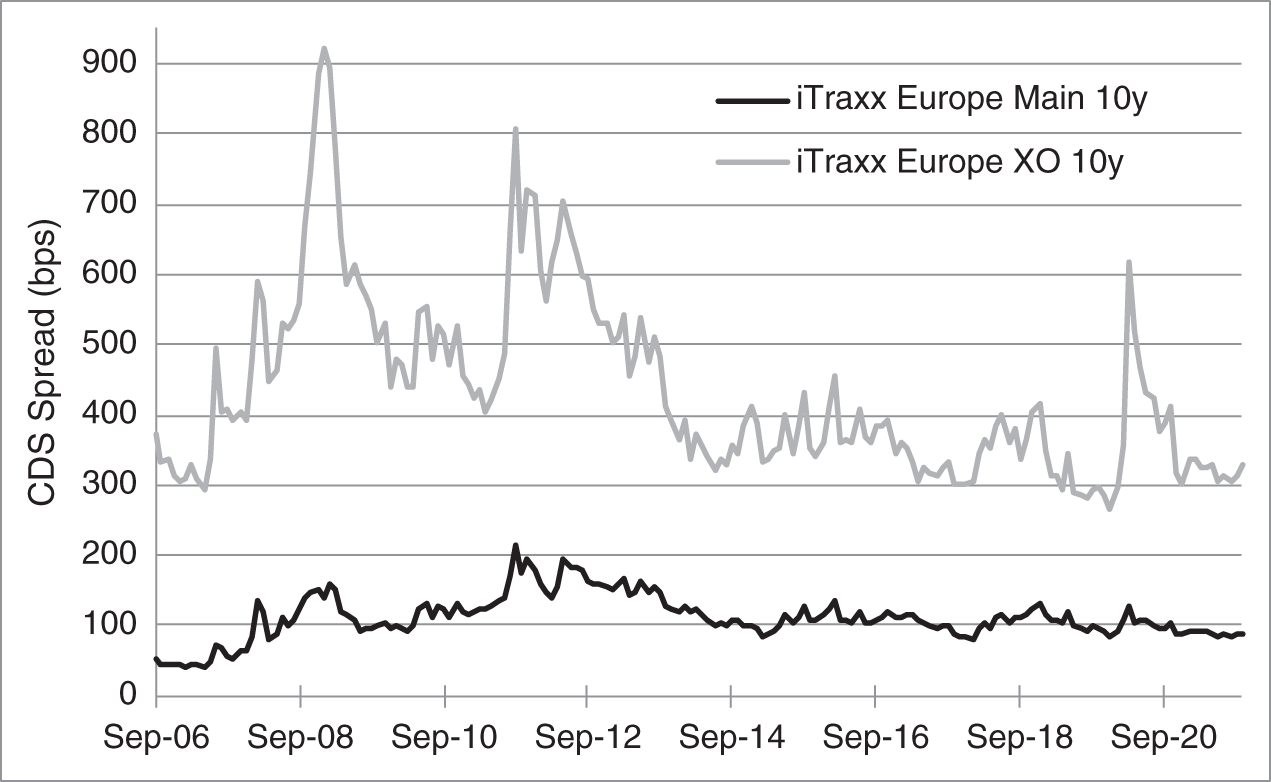
FIGURE 14.4 iTraxx Europe 10‐Year CDS Indexes.
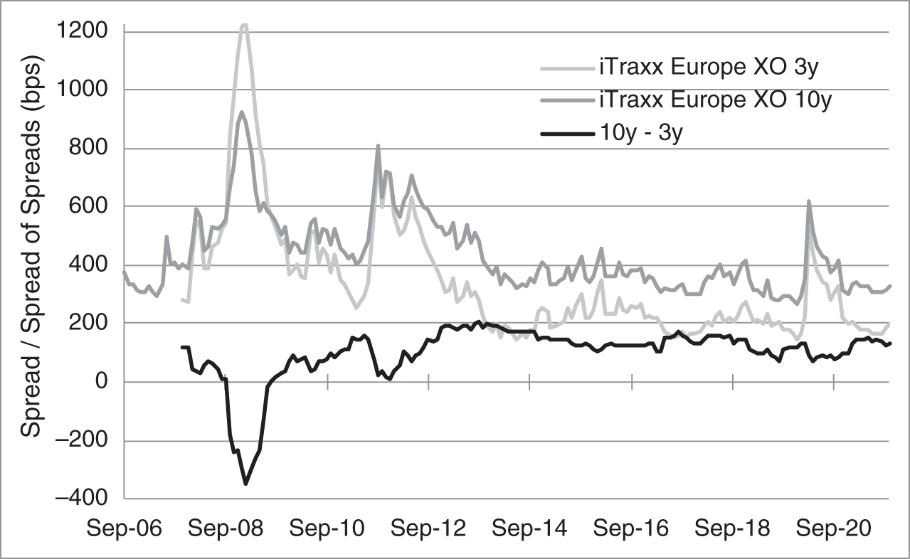
FIGURE 14.5 iTraxx Europe 10‐Year versus Three‐Year Crossover CDS Indexes.
As mentioned earlier and discussed presently, selling CDS protection very much resembles buying a bond: both the protection seller and the investor receive coupons over time and lose money in the event of a default. Many sellers of protection, therefore, choose to bear credit risk through CDS rather than bonds. One reason might be that the relatively few CDS contracts on a particular name (e.g., a five‐ and 10‐year) are more liquid than that name's many outstanding bond issues. Similarly, selling protection on an index might be a lot less costly than assembling a similarly diversified portfolio by buying individual corporate bonds. Even if an asset manager ultimately wants to hold the bonds, the fastest way to put on the position might be to sell protection and then, over time, buy the bonds and unwind the protection sold. A second reason to prefer selling protection over buying bonds might be to isolate credit risk from interest rate risk. Many insurance companies, for example, engage in replication synthetic asset transactions (RSATs), in which, for example, they buy government bonds of a maturity that suits their asset–liability management requirements and then sell protection on a credit that they like for investment purposes. A third reason, also discussed in this chapter, is that selling protection allows an investor to take risk with relatively little capital, whereas buying a bond requires that cash be available or explicitly borrowed.
Protection buyers, on the other hand, very much resemble short sellers: both pay coupons over time and win money in the event of a default. One reason to short corporate credit in CDS form is that it may be most efficient to do so, given the relatively significant trouble and expense of borrowing corporate bonds to short them. A second reason, paralleling a discussion in the previous paragraph, is that an investor might want to sell a corporate bond, but its liquidity would require a gradual, relatively slow unwind. In that case, if urgency is important, the best strategy might be to buy protection immediately in the more liquid CDS market, and then gradually sell the bond and unwind the purchased protection. A third reason to buy CDS protection is to hedge against risks that are not traded at all. For example, an entity doing business with Italian firms that have no publicly traded debt or related CDS might want to hedge against deteriorating credit conditions in that country by buying protection on Italian banks. This example has important consequences, as it implies that market participants might purchase protection on credits to which they have no direct exposure. And this, in turn, means that the amount of CDS outstanding on particular credits might exceed their outstanding debt. Back to the example, if many market participants want to hedge financial risk in Italy, the amount of CDS protection bought on Italian banks could exceed the amount of Italian bank debt outstanding.
A recent study puts the global outstanding notional amount of CDS at $9.4 trillion, split 62% in index CDS and 38% in single‐name CDS. Notional amounts are misleading indicators of outstanding risk, however, for the same reasons that apply to interest rate swaps, which are discussed in Chapter 13. Net notional outstanding then, from the same study, which nets each entity's long and short positions, is only $1.5 trillion, with two‐thirds of that in index CDS and one‐third in single‐name CDS. CDX.NA.IG and iTraxx Europe account for about 70% of traded index amounts, and the top five aforementioned CDS contracts account for more than 90% of index activity. With respect to the single‐name market, about 800 distinct names are referenced in each quarter of trading, but only about 550 of those names are referenced in every quarter. This implies that the single‐name market consists of a core group of names that are traded consistently over time and other names that trade when interest is high in their particular credit situations.13
14.6 CDS UPFRONT AMOUNTS
Before the financial crisis of 2007–2009, CDS traded like interest rate swaps; that is, the coupon changed every moment with market conditions, and standard maturities were fixed terms from the settlement date. For example, buying $1 million notional of five‐year CDS on Genworth at a spread of 558.92 basis points on August 16, 2006, was a commitment to pay $55,892 annually in exchange for compensation in the event of a Genworth default through August 16, 2011. Consequently, as is still true for interest rate swaps today (see Chapter 13), unwinding CDS trades was relatively difficult. For example, to unwind the CDS just described after one month, a trader would most like to sell protection at a fee of 558.92 basis points through August 16, 2011. But at the time of the unwind, on September 16, 2006, the most liquid or on‐the‐run five‐year CDS would mature on September 16, 2011, and might carry a spread of 490 basis points. The trader, therefore, would have to incur relatively high transaction costs to unwind the existing CDS, or would have to sell protection through the on‐the‐run CDS and manage the maturity and spread mismatch between the original and the hedging CDS.
Since the financial crisis, as part of a broader push by regulators to improve operations in this market, CDS have become more standardized. First, maturity dates are limited to pseudo‐IMM (international money market) dates, that is, the 20th days of March, June, September, or December. Thus, for example, all five‐year contracts traded between June 21, 2021, and September 20, 2021, mature on September 20, 2021; all five‐year contracts traded between September 21, 2021, and December 20, 2021, mature on December 20, 2021; etc. Second, all contracts have annual coupons of either 100 or 500 basis points, with a market determined upfront amount to compensate for the difference between the market CDS spread and the standardized coupon. Upfront amounts are described in greater detail later, but, for the present, note how these two changes in market conventions simplify the unwind of CDS. Buying a $1 million five‐year CDS on Genworth on August 16, 2021, at a spread of 558.92 actually requires making annual payments of 500 basis points or $50,000, and – as shown next – an upfront payment of $23,190. Furthermore, the contract matures on September 20, 2021. Therefore, to unwind this contract after one month, the trader can sell a still on‐the‐run CDS, that is, a CDS with a coupon of 500 basis points that matures on September 20, 2021, which exactly offsets the future cash flows of the original CDS.14 If the market upfront payment fell over the month to $13,000, then the trader suffers a loss of $10,190 relative to the original purchase price. Unwinding the contract after more time has passed can be more difficult, because the on‐the‐run contract may have changed, but some liquidity is likely still available: many market participants likely traded Genworth CDS between June 21, 2021, and September 20, 2021, and, therefore, have contracts with a coupon of 500 basis points and a maturity of September 20, 2021.
A short mathematical prelude is needed here before moving to the calculation of upfront amounts. Simple credit risk models assume a constant hazard rate, ![]() , defined such that the probability of default over a short time interval,
, defined such that the probability of default over a short time interval, ![]() years, equals
years, equals ![]() . If the hazard rate is 10% and that time interval is six months, then the probability of default over the six months is 10%/2 or 5%, and the probability of “survival,” meaning no default, is 95%. To survive over a year requires survival over both the first and second six months, which has a probability of
. If the hazard rate is 10% and that time interval is six months, then the probability of default over the six months is 10%/2 or 5%, and the probability of “survival,” meaning no default, is 95%. To survive over a year requires survival over both the first and second six months, which has a probability of ![]() . And this survival probability, in turn, implies that the probability of default over the year, whether in the first or the second six months, is
. And this survival probability, in turn, implies that the probability of default over the year, whether in the first or the second six months, is ![]() , or 9.75%. Note that breaking the one‐year time frame into two six‐month periods makes the probability of survival over the year, 90.25%, greater than 90% (100% minus the annual hazard rate of 10%): with 95% survival over the first six months, only that 95% – not the full 100% – is subject to default over the second six months. Correspondingly, the probability of default over the year, 9.75%, is less than the annual hazard rate of 10%.
, or 9.75%. Note that breaking the one‐year time frame into two six‐month periods makes the probability of survival over the year, 90.25%, greater than 90% (100% minus the annual hazard rate of 10%): with 95% survival over the first six months, only that 95% – not the full 100% – is subject to default over the second six months. Correspondingly, the probability of default over the year, 9.75%, is less than the annual hazard rate of 10%.
More generally, Appendix A14.1 shows that if the hazard rate is applied continuously, then the cumulative survival probability over ![]() years,
years, ![]() , and the cumulative default probability over
, and the cumulative default probability over ![]() years,
years, ![]() , are,
, are,
TABLE 14.10 Calculating the Upfront Amount for 100 Notional Amount of an Annual Pay Five‐Year CDS on Genworth at a Coupon of 500 Basis Points and a CDS Spread of 558.92 Basis Points, as of August 16, 2021. The Recovery Rate Is 40%. Probabilities and the Hazard Rate Are in Percent.
| Discount | Cumulative Survival | Default | |
|---|---|---|---|
| Year | Factor | Probability | Probability |
| 1 | 0.998462 | 91.099 | 8.901 |
| 2 | 0.994257 | 82.991 | 8.109 |
| 3 | 0.985062 | 75.604 | 7.387 |
| 4 | 0.973167 | 68.875 | 6.729 |
| 5 | 0.959797 | 62.744 | 6.130 |
| Hazard Rate | 9.322 | ||
| Value of Fee Leg | 21.995 | ||
| Value of Contingent Leg | 21.995 | ||
| Upfront Amount | 2.319 | ||
To illustrate the use of these equations with the same annual hazard rate of 10%, the cumulative survival probability over four years is ![]() , and the cumulative default probability is one minus that, or 33.0%. Note again that, because of the compounding of survival probabilities over many short time intervals, the four‐year survival rate of 67.0% is significantly greater than one minus four years at 10%, or 60%, and, correspondingly, the four‐year default rate of 33.0% is significantly less than 40%.
, and the cumulative default probability is one minus that, or 33.0%. Note again that, because of the compounding of survival probabilities over many short time intervals, the four‐year survival rate of 67.0% is significantly greater than one minus four years at 10%, or 60%, and, correspondingly, the four‐year default rate of 33.0% is significantly less than 40%.
Appendix A14.2 gives general, algebraic formulae for the market convention of calculating a CDS upfront amount given a quoted CDS spread. The text, however, continues with an example described in Table 14.10: 100 notional amount of a five‐year Genworth CDS as of August 16, 2021. The CDS coupon is 500 basis points; the market CDS spread is 558.92 basis points; and the assumed recovery rate is 40%.15 For simplicity, it is assumed that premium payments are annual (instead of quarterly).
The basic idea behind the market convention is as follows. First, find the hazard rate that makes the Genworth CDS “fair” in the sense that the expected discounted value of paying for protection with the CDS spread – here 558.92 basis points per year – is equal to the expected discounted value of receiving compensation in the event of default – here ![]() . This hazard rate turns out to be 9.322%. Second, using that hazard rate, find the expected discounted value to the protection buyer of paying the actual CDS coupon – here 500 basis points – instead of the CDS spread of 558.92 basis points. That value turns out to be 2.319. Hence, to buy 100 face amount of Genworth protection at a coupon of 500 basis points, when the CDS spread is actually 558.92, the protection buyer has to pay an additional 2.319 upfront.
. This hazard rate turns out to be 9.322%. Second, using that hazard rate, find the expected discounted value to the protection buyer of paying the actual CDS coupon – here 500 basis points – instead of the CDS spread of 558.92 basis points. That value turns out to be 2.319. Hence, to buy 100 face amount of Genworth protection at a coupon of 500 basis points, when the CDS spread is actually 558.92, the protection buyer has to pay an additional 2.319 upfront.
The first column of Table 14.10 lists the years of the five annual payments. The second column gives the discount factors from the LIBOR swap curve as of the pricing date. The third and fourth columns give the cumulative survival and default probabilities at the end of each year, computed with Equations (14.4) and (14.5) and a hazard rate of 9.322%. This hazard rate is shown in the table, and its derivation is given presently.
Like all CDS, the Genworth CDS in the example can be described as having two legs: a fee leg and a contingent leg. The fee leg comprises the payments of the premium from the buyer to the seller of protection. At the end of any year in which there has not been a default, the buyer in the current calculation has to pay the CDS spread of 558.92 basis points on the 100 notional amount, or 5.5892. If there is a default over the year, then the buyer has to pay the accrued coupon from the start of the year to the time of default. If, for example, the default occurred after three months, or one‐quarter of a year, the buyer would have to pay one‐fourth of the coupon, or 1.3973; if the default occurred in the middle of the year, the buyer would have to pay 2.7946. For simplicity, however, the market convention for calculating upfront amounts assumes accrual for half the period, or, in this example, for half of the year. (This assumption has less impact on the calculations in practice, because coupons are actually paid quarterly.)
Continuing with the example, then, the buyer's payment on the fee leg at the end of the first year is 5.5892 if there is no default over the year, and 2.7946 if there is. The probability of these two contingencies are reported in the table as 91.099% and 8.901%, respectively. Hence, the expected present value of this payment is,
Analogous calculations can be repeated for each of the next four years, using the appropriate survival and default probabilities and discount factors. Then, summing the results gives the present value of the fee leg, reported in Table 14.10, as 21.995.
TABLE 14.11 Calculating the Expected Discounted Value of 100 Face Amount of an Annual Pay Five‐Year 5% Genworth Bond as of August 16, 2021, at a Hazard Rate of 9.322% and a Recovery Rate of 40%.
| Expected PV Coupon | Expected PV Principal | |||
|---|---|---|---|---|
| Year | Default | No Default | Default | No Default |
| 1 | 0.222 | 4.548 | 3.555 | |
| 2 | 0.202 | 4.126 | 3.225 | |
| 3 | 0.182 | 3.724 | 2.911 | |
| 4 | 0.164 | 3.351 | 2.620 | |
| 5 | 0.147 | 3.011 | 2.354 | 60.222 |
| Total | 0.916 | 18.760 | 14.663 | 60.222 |
| Bond Price | 94.561 | |||
With respect to the contingent leg, the seller of protection pays the buyer 60 in any year that Genworth experiences a default. The expected discounted value of that contingent payment in the third year, for example, is,
Performing this calculation for each of the five years and summing the results gives the present value of the contingent leg, reported in Table 14.10, as 21.995.
Because the discounted expected values of the fee and contingent legs are equal, the hazard rate of 9.322% correctly reflects the market CDS spread of 558.92 basis points. Solving for this hazard rate in the first place requires iterating through the calculations just described. For example, after setting up the calculations in Table 14.10 as an Excel spreadsheet, the built‐in solver can be used to find the hazard rate that results in equal values for the fee and contingent legs.
The stage is now set for calculating the upfront amount such that paying this upfront amount at the initiation of the CDS and then paying a running premium of 500 basis points has the same discounted expected value as paying nothing upfront and then a running premium of 558.92 basis points. As derived previously, the expected discounted value of the fee leg making payments of 5.5892 is 21.995. It follows, then, that the value of payments of the standardized coupon of five in the fee leg is ![]() . Therefore, the required upfront payment is just the difference,
. Therefore, the required upfront payment is just the difference, ![]() , or 2.319: an upfront payment of 2.319 and a running premium of five (which is worth 19.676) has the same value as no upfront payment and a running premium of 5.5892 (which is worth 21.995).
, or 2.319: an upfront payment of 2.319 and a running premium of five (which is worth 19.676) has the same value as no upfront payment and a running premium of 5.5892 (which is worth 21.995).
A moment's reflection reveals that the upfront amount is positive whenever the CDS spread is greater than the standardized coupon. If the market CDS spread of Genworth were 450 on August 16, 2021, then the upfront amount turns out to be ![]() 2.051. Buying protection by receiving 2.051 upfront and paying a running premium of five has the same value as no upfront amount and paying a running premium of 4.50.16
2.051. Buying protection by receiving 2.051 upfront and paying a running premium of five has the same value as no upfront amount and paying a running premium of 4.50.16
This section concludes by emphasizing that the quoting of an upfront amount from a CDS spread is only a convention, like the relationship between price and yield‐to‐maturity. Market participants form their own views on upfront amounts at which they are willing to trade CDS. They may not be willing, for example, to assume a particular recovery rate or that the hazard rate is constant over time. But they all use the accepted market conventions to calculate upfront amounts from a quoted CDS spread or vice versa.
14.7 CDS‐EQUIVALENT BOND SPREAD
The credit spreads defined earlier in the chapter are all measures of bond return assuming no default. An alternative approach, the CDS‐equivalent bond spread, accounts for default and recovery and is computed along the lines of the previous section. The basic idea is to find the hazard rate such that the market price of the bond equals the expected discounted value of its cash flows. Then, the bond's CDS‐equivalent spread is the CDS spread corresponding to that hazard rate. To illustrate, say that the market price of a five‐year, 5% (annual pay) bond on Genworth is 94.561 as of August 16, 2021. It is shown next that the expected discounted value of that bond's cash flows equals that market price if the hazard rate is 9.322%. Furthermore, from Table 14.10, the five‐year CDS spread at a hazard rate of 9.322% is 558.92 basis points. Therefore, the CDS‐equivalent spread of this five‐year, 5% bond is 558.92 basis points. In other words, the credit risk implied by the bond's market price is the same as that implied by a five‐year CDS at a spread of 558.92 basis points. This spread depends on the restrictive assumption that the hazard rate is constant. The calculation of expected discounted values, while seeming to imply risk neutrality, is not as restrictive as it seems: the hazard rate can be considered “risk‐neutral” so that it prices fixed income securities without necessarily reflecting real‐world probabilities. (This distinction is discussed in Chapter 7.)
Appendix A14.4 gives the algebra for calculating the expected discount value of a bond's cash flows given a hazard rate. The text, however, continues with pricing 100 face amount of an annual pay, five‐year, 5% Genworth bond as of August 16, 2021, and the results are summarized in Table 14.11. Because the bond's assumed market price is consistent with a hazard rate of 9.332%, which is the hazard rate in Table 14.10, the cumulative survival and default probabilities from that table can be used here. Also, because the pricing dates are the same, the discount factors from that table can be used here as well.
Along the lines of the previous section, the expected value of a bond's coupon in a given year is half of its value times the probability of default over the year plus its value times the probability of no default over the year. The discounted expected value of the first coupon of the 5% Genworth bond, for example, is as in Equation (14.6), but with the bond coupon of 5.00 replacing the CDS spread payment of 5.5892,

The two components of this coupon's expected discounted value are given in the second and third columns of the first row of Table 14.11. The next rows of the table repeat this calculation for subsequent coupon payments, using the appropriate discount factors, cumulative survival probabilities, and cumulative default probabilities from Table 14.10. Summing the results, the total discounted expected value of the bond's coupons is ![]() .
.
With respect to principal, if there is a default in any year, then the principal received is the face amount times the recovery rate. The discounted expected value of principal received in the third year, for example, is the three‐year discount factor times the probability of default in year three times the recovery on 100 face amount,
which is the value given in the fourth column, third row, of Table 14.11. (Note that, in Equation (14.9), the bondholder receives 40, while in Equation (14.7), the buyer of protection receives a default compensation of 60.) The table uses the equivalents of Equation (14.9) to calculate the rest of the fourth column.
If there is no default up to and including maturity, the bond pays its full principal amount. The expected discounted value of this cash flow is,
and is given in the year five row and in the rightmost column of Table 14.11.
Finally, adding together the four components of the bond's expected discounted value from the table, the bond's price is 94.561. Hence, because the bond is fairly priced using a hazard rate of 9.322%, and because that hazard rate corresponds to a CDS spread of 558.92 basis points (from the previous section), this bond's CDS equivalent spread is 558.92 basis points.
This section now compares the CDS‐equivalent bond spread just explained with the bond spread discussed already. First, Appendix A14.3 shows that the CDS spread is approximately equal to the hazard rate times one minus the recovery rate. Mathematically, letting ![]() denote the CDS spread; letting
denote the CDS spread; letting ![]() denote the hazard rate, as before; and letting
denote the hazard rate, as before; and letting ![]() denote the recovery rate,
denote the recovery rate,
In the context of Table 14.10, for example, the approximation predicts a CDS spread of 9.322% times (1 − 40%), or 559.32 basis points, while the actual spread is a very close 558.92 basis points.
Second, Appendix A14.5 shows that,
where ![]() is the bond spread, and
is the bond spread, and ![]() is the recovery rate as a percentage of market value. To this point the chapter has assumed par recovery, that is, bond recovery rates are best modeled as a fixed percentage of face amount. Market recovery, by contrast, which is used to derive Equation (14.12), assumes that recovery is a fixed percentage of market value. Say that two bonds were sold by the same issuer with the same seniority, but one of the bonds has a much longer maturity and trades at a larger price discount or premium, depending on the level of rates and spreads. In the event of default, will the two bonds recover the same amount – as assumed by par recovery – or will the longer‐term bond's recovery reflect its greater discount or premium – as assumed by market recovery? Par recovery is the more common assumption and is better supported by empirical evidence.17
is the recovery rate as a percentage of market value. To this point the chapter has assumed par recovery, that is, bond recovery rates are best modeled as a fixed percentage of face amount. Market recovery, by contrast, which is used to derive Equation (14.12), assumes that recovery is a fixed percentage of market value. Say that two bonds were sold by the same issuer with the same seniority, but one of the bonds has a much longer maturity and trades at a larger price discount or premium, depending on the level of rates and spreads. In the event of default, will the two bonds recover the same amount – as assumed by par recovery – or will the longer‐term bond's recovery reflect its greater discount or premium – as assumed by market recovery? Par recovery is the more common assumption and is better supported by empirical evidence.17
In short, CDS and bond spreads are not equivalent, and the consensus in favor of the par recovery assumptions argues in favor of preferring the CDS spread. Furthermore, at high hazard rates and low bond prices, the CDS spread is significantly greater than the bond spread. To illustrate, recall from Tables 14.10 and 14.11 that the five‐year 5% Genworth bond, at a hazard rate of 9.322% and a price of 94.561, has a CDS spread of 559 basis points. From the data in these tables, it can also be computed that its bond spread is a similar 551 basis points.18 However, if the hazard rate is a much higher 16.70%, then the bond price is 80.688; the CDS spread is 1,000 basis points; and the bond spread is a much lower 932 basis points. (These computations are also left as an exercise for the reader.) Intuitively, by assuming too low a recovery for discount bonds, bond spreads have to be lower to reproduce seemingly high market prices.
14.8 CDS‐BOND BASIS
Credit risk today is traded in both the corporate debt market and in the CDS market. It is natural to ask, therefore, whether a particular credit trades at the same price in both markets or is cheaper in one market than the other. If the latter, then there might be relative value trading opportunities to buy in one market and sell in the other.
Table 14.12 sets the stage with a simplified relationship between selling CDS protection on a particular credit and buying a bond of that same credit, financed in the repo market.19 The table is a simplification by assuming that i) the CDS contract has an upfront payment of zero, that is, the CDS coupon equals the CDS spread; ii) the corporate bond is priced at par; and iii) the CDS and the underlying bond mature on the same date. Under these assumptions, the table shows that selling CDS protection is equivalent to buying a bond and financing its purchase with term repo to the bond's maturity. More specifically, the cash flows from selling 100 notional of CDS are: zero today; the spread ![]() on 100 until the earlier of default or maturity;
on 100 until the earlier of default or maturity; ![]() if and when the bond defaults; and zero if the bond matures without a default. The cash flows from buying 100 face amount of the bond at a price of par are
if and when the bond defaults; and zero if the bond matures without a default. The cash flows from buying 100 face amount of the bond at a price of par are ![]() 100 today; the coupon rate
100 today; the coupon rate ![]() on the face amount to the earlier of default or maturity;
on the face amount to the earlier of default or maturity; ![]() if and when the bond defaults; and 100 if the bond matures without a default. Finally, the cash flows from borrowing the bond's purchase price through repo are 100 today;
if and when the bond defaults; and 100 if the bond matures without a default. Finally, the cash flows from borrowing the bond's purchase price through repo are 100 today; ![]() on 100 until the earlier of default or maturity; and
on 100 until the earlier of default or maturity; and ![]() 100 at the earlier of default or maturity. (To clarify these repo cash flows, note that, if a bond defaults, the borrower has to unwind the repo position by paying off the 100 loan amount, which then ends interest payments on the loan.) Finally, adding the cash flows from purchasing the bond and selling the repo gives the “Total” row, which exactly matches the cash flows of selling CDS protection so long as
100 at the earlier of default or maturity. (To clarify these repo cash flows, note that, if a bond defaults, the borrower has to unwind the repo position by paying off the 100 loan amount, which then ends interest payments on the loan.) Finally, adding the cash flows from purchasing the bond and selling the repo gives the “Total” row, which exactly matches the cash flows of selling CDS protection so long as ![]() .
.
TABLE 14.12 A Simplified Arbitrage Relationship Between Selling Protection on a Credit and Buying a Bond on That Same Credit, Financed by Repo.
| Today | Interim (%) | Default | Maturity/No Default | |
|---|---|---|---|---|
| Sell CDS Protection | 0 | 0 | ||
| Buy Par Bond | 100 | |||
| Sell Repo | 100 | |||
| Total | 0 | 0 |
The CDS‐bond basis refers to the difference between the CDS spread and some measure of the bond's spread over riskless rates. In the simplified setting of Table 14.12, where the bond spread is the difference between the par coupon and the matching‐term repo rate, the CDS‐bond basis is ![]() . If the basis is positive, then
. If the basis is positive, then ![]() , which means that the bond is rich, or that it has a low spread relative to the CDS spread. Put another way, selling CDS protection earns more than buying the bond. If the basis is negative, then
, which means that the bond is rich, or that it has a low spread relative to the CDS spread. Put another way, selling CDS protection earns more than buying the bond. If the basis is negative, then ![]() , which means that the bond is cheap relative to the CDS spread, and that buying the bond earns more than selling CDS protection. In either case, when the basis is not zero, an arbitrage opportunity is available. If positive, execute a positive basis trade, that is, sell protection, short the bond, and buy the repo, to lock in
, which means that the bond is cheap relative to the CDS spread, and that buying the bond earns more than selling CDS protection. In either case, when the basis is not zero, an arbitrage opportunity is available. If positive, execute a positive basis trade, that is, sell protection, short the bond, and buy the repo, to lock in ![]() per period until the earlier of default or maturity. And if the basis is negative, execute a negative basis trade, that is, buy protection, buy the bond, and sell the repo, to lock in
per period until the earlier of default or maturity. And if the basis is negative, execute a negative basis trade, that is, buy protection, buy the bond, and sell the repo, to lock in ![]() per period.
per period.
Crucial to these arbitrage arguments is that the term of the repo equal the maturity of the bond and the CDS. In a negative basis trade, for example, selling overnight – rather than term – repo exposes a trader to financing risk: the overnight repo rate might increase dramatically or repo funding might be withdrawn completely, either because the bond's creditworthiness has deteriorated, because general financing supply has tightened, or because the trader's own credit has come under stress. In any of these scenarios, the trader might very well be forced to unwind the position at a loss, that is, when the bond has become even cheaper relative to CDS. Similarly, in executing a positive basis trade with overnight repo, the financing risk is not being able to continue to borrow the bonds in order to maintain the short position.
In practice, because there is no market for very long‐term corporate repo, it is nearly impossible to execute a basis trade without bearing financing risk. Therefore, despite arbitrage arguments like Table 14.12, there is a fundamental difference between CDS and levered bond positions: CDS positions have implicit financing to maturity, while levered bond positions are inherently subject to financing risk.
Outside the simplified setting of Table 14.12, market participants compute the CDS‐bond basis using different measures of a bond's spread, like yield spread, bond spread, asset swap spread, and CDS‐equivalent bond spread. The advantages and disadvantages of each of these is discussed previously, but all of these measures can be misleading in the context of the CDS‐bond basis. Without a term‐repo rate, any measure of the basis ignores the financing risk in a CDS versus levered bond arbitrage trade.
A lot of money was lost in negative basis trades through the financial crisis of 2007–2009. As funding conditions became more difficult, CDS‐bond bases moved negative, reflecting the difficulty of going long credit risk with levered bond positions relative to selling CDS protections. Some traders, however, saw these negative bases as trading opportunities, which turned into nightmares as funding conditions deteriorated even further. Over the crisis, in fact, the investment‐grade index CDS‐bond basis fell from about zero to negative 250 basis points.
Figure 14.6 shows the CDS‐bond basis for French and Italian government bonds from January 2006 to October 2021. The basis is defined here as the difference between the five‐year CDS spread and the five‐year government bond yield spread over Germany. By way of economic backdrop, the European sovereign debt crisis ran from the end of 2009 to 2012, during which time the finances of both banks and governments in the so‐called “peripheral” countries (e.g., Greece, Italy, Portugal, and Spain) came under pressure. Later, in the fall 2018, European Union and Italian government officials squabbled over Italy's proposed budget, which did not comply with existing fiscal rules. The figure shows that the sovereign Italian CDS‐bond basis became significantly negative during both of these stressful periods. As in the financial crisis of 2007–2009, repo lenders became reluctant to fund Italian government bonds, pushing up their spreads and pushing their CDS‐bond basis into negative territory. In fact – though not shown in the figure – spreads of Italian to German government bonds rose to over 600 basis points during the sovereign debt crisis, and to nearly 300 basis points during the budget standoff. By contrast, French government credit exhibited a positive CDS‐bond basis during the sovereign debt crisis. French over German spreads did rise to a peak of about 100 basis points at that time, but the bigger story was the difficulty of borrowing and shorting French government bonds, at least in part because the European Central Bank was aggressively buying European sovereign debt. In any case, the resulting upward pressure on French government bond prices resulted in a significantly positive CDS‐bond basis.20 Finally, more recently, funding stresses during the COVID pandemic and economic shutdowns drove both Italian and French government CDS‐bond bases somewhat negative.

FIGURE 14.6 CDS‐Bond Basis for French and Italian Sovereign Debt, January 2006 to October 2021.
14.9 HAZARD‐ADJUSTED DURATION AND DV01
The durations of bonds with credit risk are often calculated along the lines of Chapter 4, that is, cash flows are assumed to be paid on schedule, but are discounted at higher rates, typically at benchmark rates plus a credit spread or a term structure of credit spreads. Calculated this way, however, duration can be misleading for bonds with significant credit risk. For these bonds, expected cash flows are much earlier than scheduled cash flows and, consequently, their durations are correspondingly shorter.
The simple hazard‐rate framework presented earlier can be used to calculate a hazard‐adjusted duration (HAD) that accounts for the expected timing of cash flows given default. Along the lines of Table 14.11, given a benchmark rate curve and a recovery rate, find the hazard rate for which the expected discounted value of the bond's cash flows equals its market price. Then, shift the benchmark rate curve down and reprice the bond, using the same recovery and hazard rates. Finally, use the resulting price difference or percentage price difference to compute the hazard‐adjusted DV01 or duration, respectively.
To illustrate the difference between the conventional and hazard‐adjusted approaches, Figure 14.7 graphs conventional and hazard‐adjusted durations for bonds of various terms at two different hazard rates. The benchmark rate curve is flat at 2%, and the recovery rate is fixed at 40%. The hazard rate is either 5% or 10%, which, given the 40% recovery rate, corresponds approximately to CDS spreads of 300 and 600 basis points, respectively. All bonds are priced using the constant hazard‐rate model, and HADs are computed as described in the previous paragraph. Conventional durations are calculated by finding the fixed spread to the benchmark curve that correctly prices each bond, and then shifting the benchmark curve and repricing each bond, keeping its spread constant.

FIGURE 14.7 Conventional Vs. Hazard‐Adjusted Durations.
Bonds with a higher hazard rate have higher spreads and, therefore, lower durations than bonds with a lower hazard rate. The striking message of Figure 14.7, however, is that HADs can be significantly below conventional durations, particularly for larger hazard rates and longer terms. For 10‐year bonds at a hazard rate of 5%, the conventional duration is 7.7 and the HAD is 7.3, while at a hazard rate of 10%, the durations are 7.3 conventional and 6.4 HAD. For 30‐year bonds at a hazard rate of 5%, the conventional duration is 15.3 and the HAD is 12.8, while at a hazard rate of 10%, the durations are 13.2 conventional and 8.7 HAD.
14.10 SPREAD DURATION AND DV01
When trading or investing in credit portfolios, it is natural to measure the sensitivity of bond prices to changes in credit spreads. The standard measures, spread duration and spread DV01, shift the spread, keeping the benchmark curve and cash flows the same, calculate a new price, and then calculate a duration or DV01. Because rates used for discounting in this context are the sum of the benchmark rates and spreads, shifting the benchmark rate by one basis point results in the same price sensitivity as shifting the spread by one basis point, that is, spread durations and DV01s are the same as durations and DV01s with respect to interest rate changes. These spread sensitivities can still be useful, however, in a portfolio context. In a portfolio of government bonds, interest rates swaps, and corporate bonds, for example, spread DV01 with respect to swap spreads can be found by shifting spreads for swaps and corporate bonds only, while spread DV01 with respect to corporate spreads can be found by shifting spreads for corporate bonds only.
It is very common in the corporate bond setting to measure spread risk with duration times spread, or DTS, instead of spread duration. This methodology is based on the empirical regularity that changes in the spread of a corporate bond are proportional to the spread itself. Consider, for example, bonds A and B, which have spread durations of five and four years, and which trade at spreads of 100 and 250 basis points, respectively. Under the usual duration assumptions of parallel shifts, bond B has spread risk of 4/5 or 80% of that of bond A. But empirical evidence suggests that if the spread of bond A increases by 10%, that is, 10 basis points from 100 to 110, then the spread of bond B also increases by 10%, that is, 25 basis points from 250 to 275. In this case, after these spread changes, by the definition of duration, the percentage change of bond A is ![]() , and the percentage change of bond B is
, and the percentage change of bond B is ![]() . Hence, bond B is actually twice as risky as bond A. This is reflected in their DTS:
. Hence, bond B is actually twice as risky as bond A. This is reflected in their DTS: ![]() for bond A, and
for bond A, and ![]() for bond B.
for bond B.
Price sensitivity to spreads can also be computed using the hazard‐rate model described in this chapter. Risky DV01 refers to the change in the value of a CDS contract for a one‐basis‐point change in the CDS spread. This can be computed, of course, by finding the hazard rate that changes the CDS spread by one basis point, recomputing the value of the CDS, and calculating the risky DV01. An equivalent bond metric can be computed similarly: find the hazard rate that changes the CDS‐equivalent bond spread by one basis point, recompute its price, and calculate a DV01.
14.11 CDS SETTLEMENT AUCTIONS
Two challenges typical in the settlement of derivatives trades apply just as well to CDS. First, requiring that all protection buyers physically settle contracts leaves them open to a squeeze. As discussed earlier, protection buyers do not necessarily own the underlying bonds and the supply of bonds eligible for delivery might be subject to manipulation. Second, bond prices may not be readily observable for the purpose of cash settlement, because corporate bond liquidity – even if satisfactory in normal times – may be quite limited through a default. Industry‐run settlement auctions are designed to cope with both of these fundamental challenges.
TABLE 14.13 List of Deliverables for Hertz Corporation CDS Auction, June 23, 2020.
| Description | Maturity |
|---|---|
| 4.125% Sr. Notes | 10/15/2021 |
| 7.625% Sr. Secured 2nd Priority Notes | 06/01/2022 |
| 6.250% Sr. Notes | 10/15/2022 |
| 5.500% Sr. Notes | 03/30/2023 |
| Letter of Credit Disbursements | 12/18/2023 |
| 5.500% Sr. Notes | 10/15/2024 |
| 7.125% Sr. Notes | 08/01/2026 |
| 6.000% Sr. Notes | 01/15/2028 |
Hertz filed for bankruptcy on May 22, 2020, and, on June 24, 2020, an auction was held to settle CDS referencing Hertz. Some physical settlement took place as part of the auction, and the final auction price of 26.375 was used for cash settlement. This section describes the CDS auction process in the context of this Hertz CDS auction.21
A single‐name CDS contract specifies reference obligations of the reference entity, together with a set of rules, that determine whether an event of default has occurred and, if so, which bonds are deliverable, or eligible to be delivered, for the purposes of physical settlement. The final list of deliverable obligations into the Hertz CDS auction is given in Table 14.13.
The auction itself is divided into two phases. In phase one, participating dealers submit i) bids and offers for purchase and sale of deliverable obligations, with a predefined quotation size and maximum bid‐offer spread; and ii) physical settlement requests. Table 14.14 lists the bids and offers of the dealers in the Hertz auction, with the bids sorted in descending order and the offers in ascending order. An inside market midpoint (IMM) is determined from these bids and offers as follows. First, discard all rows with crossing or touching markets (i.e., where the bid price exceeds or equals the offer price). In Table 14.14, the first four rows constitute crossing or touching markets, and are discarded. Second, using the top half of the remaining rows (rounded up, if necessary), compute the average of the bids and offers and round to the nearest eighth per 100 face amount. In Table 14.14, the bottom six rows remain. Therefore, using only the top three rows, the average of the bids and offers, which are bolded, is 25.333, which, rounded to the nearest eighth, gives an IMM of 25.375.
TABLE 14.14 Dealer Initial Markets, Hertz Corporation CDS Auction, June 24, 2020.
| Dealer | Bid | Offer | Dealer |
|---|---|---|---|
| Citigroup | 26.0 | 22.5 | Morgan Stanley |
| Credit Suisse | 26.0 | 24.0 | Barclays |
| Deutsche Bank | 26.0 | 24.5 | Goldman Sachs |
| RBC Capital Markets | 25.5 | 25.5 | Bank of America |
| BNP Paribas | 24.5 | 26.0 | J.P. Morgan Securities |
| J.P. Morgan Securities | 24.0 | 26.5 | BNP Paribas |
| Bank of America | 23.5 | 27.5 | RBC Capital Markets |
| Goldman Sachs | 22.5 | 28.0 | Citigroup |
| Barclays | 22.0 | 28.0 | Credit Suisse |
| Morgan Stanley | 20.5 | 28.0 | Deutsche Bank |
| Inside Market Midpoint | 25.375 | ||
Turning to the second part of phase one of the auction, Table 14.15 shows the physical settlement requests of the participating dealers. These requests must match the direction and size of their respective net CDS positions. Goldman Sachs and its clients, for example, by offering to deliver 140.0 million face amount of deliverable obligations, must, on net, have bought protection on at least 140.0 million CDS notional amount. Put another way, Goldman and its clients are requesting to collect on their having bought a net of 140.0 million notional amount of CDS by delivering 140.0 million face amount of deliverable obligations and receiving $140 million. J.P. Morgan Securities and its clients, on the other side, by bidding to take 20.0 million of deliverable obligations, must, on net, have sold protection on at least 20.0 million CDS notional amount. They are requesting to settle their CDS obligations by taking delivery of 20.0 million of deliverable obligations and paying $20 million. Taking the physical settlement requests all together, there are total requests to sell or deliver $143.525 million face amount and total requests to buy or take delivery on $42 million, leaving a net open interest (NOI) to sell of $111.525 million.
Before proceeding to phase two of the auction, a note is made of adjustment amounts. To provide an incentive for dealers to submit competitive bids and offers, dealers are penalized for submitting off‐market bids and offers, where “off‐market” is judged relative to the IMM and NOI. More specifically, in the case of the Hertz auction, there was a NOI to sell and the IMM was 25.375. It follows from Table 14.14 that the bids and offers of Citigroup, Credit Suisse, and Deutsche Bank at 26.0–28.0, and those of RBC Capital Markets at 25.5–27.5, were too high in a market where there were more sellers than buyers. Therefore, these dealers had to pay adjustment amounts equal to the difference between their above‐market bids and the IMM times the quotation amount: $2 million × (26.0 − 25.375)/100 or $12,500 for Citigroup, Credit Suisse, and Deutsche Bank, and $2 million × (25.5 − 25.375)/100, or $2,500 for RBC Capital Markets. In phase one auctions with NOI to buy, adjustment amounts are levied on dealers with bids and offers below the IMM.
TABLE 14.15 Physical Settlement Requests, Hertz Corporation CDS Auction, June 24, 2020. Amounts Are in $Millions.
| Dealer | Size |
|---|---|
| Offers | |
| Bank of America | 0.0 |
| BNP Paribas | 3.525 |
| Citigroup | 10.0 |
| Deutsche Bank | 0.0 |
| Goldman Sachs | 140.0 |
| Morgan Stanley | 0.0 |
| RBC Capital Markets | 0.0 |
| Total Sell Requests | 143.525 |
| Bids | |
| Barclays | 7.0 |
| Credit Suisse | 15.0 |
| J.P. Morgan Securities | 20.0 |
| Total Buy Requests | 42.0 |
| Net Open Interest (Sell) | 111.525 |
Phase two of the auction takes place a few hours after the results of phase one. The purpose of phase two is to determine a final auction price, defined as the clearing price for the NOI established in phase one. In phase two, market participants – including, but not limited to the participating dealers in phase one – submit limit orders to buy, if the NOI was to sell, or limit orders to sell, if the NOI was to buy. Furthermore, to ensure the sensible result that the final auction price not be too high relative to the IMM if the NOI is to sell, or not be too low relative to the IMM if the NOI is to buy, limit order prices are constrained by a cap amount, usually set to half the maximum bid‐offer spread in phase one. In the Hertz auction, the cap amount was half of two, or one. And, because there was a NOI to sell, the limit orders to buy in phase two were constrained to be less than or equal to the IMM of 25.375 plus the cap amount of one, or 26.375.
TABLE 14.16 Goldman Sachs Limit Orders, Hertz Corporation CDS Auction, June 24, 2020. Amounts Are $Millions.
| Bid Price | Size |
|---|---|
| 26.375 | 42 |
| 25.000 | 10 |
| 24.000 | 10 |
| 23.750 | 5 |
| 23.500 | 24 |
| 23.250 | 10 |
| 23.000 | 23 |
| 22.500 | 2 |
| 20.000 | 14 |
Table 14.16 shows the limit orders to buy submitted by Goldman Sachs in phase two of the Hertz auction. On behalf of itself and its customers, Goldman Sachs bid to purchase $42 million face amount at a price of 26.375; an additional $10 million at a price of 25.000; and so forth. Note that bids from the initial market in phase one of the auction carry over into this phase, so that Goldman Sachs' bid at 22.5 for the predefined size of $2 million in Table 14.14 appears as the penultimate row of Table 14.16.22
All of the limit orders to buy Hertz bonds are collected and ordered by price, from high to low. Then, following the rules of a Dutch auction, the final auction price is set such that the quantity of limit orders to buy at that price or above matches the $111.525 million NOI to sell. In the Hertz auction, at the highest allowable bid price of 26.375, there were limit orders to purchase $118.50 million face amount, which is more than the NOI available for sale. Therefore, the final auction price was set at 26.375 and all bidders at that price were allocated a pro rata amount of the available $111.525 million. Goldman Sachs, for example, with its limit order to buy $42 million at 26.375, was able to purchase $42 million × $111.525/$118.50, or $39.528 million face amount through the auction.
To summarize, the auction had two outcomes. First, $143.525 million face amount of deliverable Hertz bonds were sold by the dealers or their customers in the “Offers” part of Table 14.15 at a price of 26.375 to the dealers or their customers in the “Bids” part of the table – $42 million – and to the market participants awarded allocations in phase two of the auction – $111.525 million. Second, all Hertz CDS settled at the final auction price of 26.375. CDS counterparties who chose cash settlement used this final price as the recovery amount, that is, protection buyers received from protection sellers the notional amount of their CDS × (100% − 26.375%), or 73.625%. Counterparties who chose physical settlement worked through their dealers as follows. Protection buyers delivered deliverable obligations of their choice for 26.375 and received a cash settlement of 73.625, for total proceeds of 100. Protection sellers paid 26.375 for any bond delivered to them and paid a cash settlement of 73.625, again, for total proceeds of 100.
This section concludes by noting that, while CDS auctions have generally been successful in settling at reasonable final prices, success is not assured. A recent example of failure was the auction to settle Europcar Mobility Group CDS on January 13, 2021. Just before the auction, deliverable bonds were trading at about 70, and phase one of the auction resulted in an IMM of 73 and a NOI to buy €43.3 million. But in phase two, limit orders to sell totaled only €35.9 million. Hence, with no price high enough to match limit sell orders to the NOI to buy, the final auction price, by rule, was set to 100. Buyers of CDS protection received nothing. Some commentators attributed the lack of limit sell orders to the fact that Europcar restructuring agreements prevented many bondholders from selling their bonds through the CDS auction. Other commentators, however, claimed that there were more than enough bonds available to cover the NOI, but potential sellers simply did not show up at the auction.23
14.12 OPPORTUNISTIC CDS STRATEGIES
In theory, CDS traders take the behavior of debt issuers as given, and debt issuers essentially ignore CDS trading on their obligations. In practice, however, because of the complexities of CDS contracts (e.g., specifying events of default; defining reference entities and deliverable obligations; setting rules for settlement auctions), both CDS traders and issuers have occasionally tried to profit from crossing the lines separating their respective markets. These instances have been called opportunistic CDS strategies.
A particularly well‐known example is the case of the real estate company, Hovnanian, and its “manufactured default.” In February 2018, Hovnanian and an asset manager that had bought over $300 million of protection on Hovnanian conducted the following transactions:
- The asset manager loaned Hovnanian a significant sum at below‐market rates.
- Hovnanian conducted a bond exchange offer, in which it issued new, very long‐term debt that would sell at a significant discount, given its relatively low credit rating; and in which some of its higher‐priced outstanding bonds were purchased by one of its own subsidiaries.
- Hovnanian committed to skip the coupon payment on its bonds owned by that subsidiary. This default would not trigger cross‐default provisions, but would trigger a credit event with respect to Hovnanian CDS.24
Through these transactions, Hovnanian was able to borrow at advantageous rates, and the asset manager, if the credit event occurred, would benefit not only from the triggering of its long CDS position, but also from the issuance of the low‐priced bond issue, which, because it was deliverable into the CDS, would lower the CDS settlement auction price and increase the payout to protection buyers. While Hovnanian did skip the coupon payment per its commitment, the company ultimately reversed course and paid before the end of the 30‐day grace period. Pressure from regulators and from asset managers who had sold protection on Hovnanian, along with a settlement between the asset managers on both sides of the CDS, led to the abandonment of this manufactured default.
The Hovnanian case threatened confidence in the integrity of the definition of “default” in the CDS market. In response, ISDA changed the definition of “failure to pay” to include the language, “it shall not constitute a Failure to Pay if such failure does not directly or indirectly either result from, or result in, a deterioration in the creditworthiness of financial condition of the Reference Entity.”25
While this change in definition is likely to eliminate some opportunistic CDS strategies, other possibilities remain. With respect to the buyers of CDS protection influencing default, consider the case of the telecommunications company, Windstream. In 2015, in the course of a restructuring, the company seems to have violated an existing bond covenant. No one objected until 2017, however, when a hedge fund bought some of the bonds and sued to put the company into default. Many market participants believe that the hedge fund bought CDS protection on Windstream, bought the bonds, and then sued to collect on the CDS. And the hedge fund did prevail in court, despite other bondholders' willingness to waive the alleged covenant violation. In this case then, not only did the event of default not reflect underlying credit conditions, but CDS buyers also seem to have precipitated that default.26
Opportunistic strategies seem also to have been pursued by sellers of CDS protection. In 2018, an asset manager, widely believed to have sold protection on the publishing company, McClatchy, made the following agreement with the company. The asset manager would buy newly issued bonds from a subsidiary of McClatchy, with the proceeds used to refinance (and extinguish) the existing bonds of McClatchy itself. Because outstanding CDS included McClatchy, but not its subsidiary, as reference entities, McClatchy CDS would be “orphaned” – without any underlying debt, McClatchy could not possibly default. Furthermore, protection buyers would still have to make premium payments. News of this agreement dramatically reduced the value of protection, generating profits for sellers of protection. As it turned out, the proposed deal did not go through and, in early 2020, McClatchy filed for bankruptcy. And, in the subsequent CDS auction, the final price was two; that is, McClatchy CDS eventually paid 98 cents on the dollar.27
As a final example of opportunistic CDS strategies, in this instance with the issuer as first mover, consider the case of Sears Holding Corp. At the time of its bankruptcy, in late 2018, there was a lot of CDS outstanding not on the holding company, but on its subsidiary, Sears Roebuck Acceptance Corp (SRAC). But relative to SRAC CDS, there was relatively little SRAC debt outstanding, perhaps about $200 million. Therefore, CDS buyers were willing to pay a premium to buy SRAC debt: they could thus ensure having enough bonds to sell into the settlement auction, which, in turn, would keep the final auction price low and default compensation high. Recall that in the Europcar auction, with too few submitted limit sell orders, the final auction price was 100 and protection buyers received nothing. In any case, Sears realized that – because of the CDS market – the market value of SRAC bonds far exceeded the expected discounted value of their cash flows and offered to sell a previously overlooked $900 million of intercompany SRAC notes. CDS buyers were outbid in this sale, however, by CDS sellers – who wanted to prevent these SRAC bonds from being delivered into the settlement auction. In the end, however, to stop the back‐and‐forth litigation, CDS buyers and sellers came to a settlement on their own.
There are several examples of opportunistic CDS strategies other than the ones described here, but at least two lessons emerge. First, market participants need to be aware of special situations that could cause final recovery to differ from expectations. Second, if opportunistic strategies were ever to dominate trading, many market participants might very well abandon the market, believing that it no longer offered straightforward transfers of credit risk.
14.13 CASE STUDY: THE LONDON WHALE
In the first half of 2012, JPMorgan Chase (JPM) lost more than $6 billion on its “London Whale” trades. With assets at the time of over $2 trillion and 2012 income of $21 billion, the loss in no sense endangered the bank, but it was large and embarrassing. In this chapter, the case is used to explain more fully the workings of index CDS and CDS tranches, though other lessons include the need to define the purpose and scope of hedging programs and the importance of sizing trades so as not to “become the market.”28
Index CDS and Tranches
The important instruments for understanding the events of the case are CDX.NA.IG.9 and its tranches. As described earlier in the chapter, CDX.NA.IG is an equally weighted index of 125 investment‐grade North American entities. The “.9” indicates a particular series of this index, which came out in the third quarter of 2007. Hence, 10‐year protection on this index expired in December 2017 and five‐year protection in December 2012. As the London Whale events unfolded in the first quarter of 2012, 10‐year CDS on this index matured in just under six years, and five‐year CDS on the index matured in just under a year.
As of April 2012, four of the 125 names in CDS.NA.IG.9 had experienced credit events during the financial crisis of 2007–2009 and, therefore, had dropped out of the index: CIT, a subprime mortgage lender; WAMU, a Savings and Loan Association; Fannie Mae, a government sponsored mortgage agency; and Freddie Mac, a government sponsored mortgage agency. Table 14.17 shows the impact of these four credit events on the index. The second column shows the final price in the CDS auction for each of the names. To understand the third column, consider $125 million original notional amount of the index, which would include $1 million notional amount in each of the underlying 125 names. Given an auction price of 68.125 for CIT obligations, $1 million notional amount of CDS on CIT lost ![]() × $1 million, or $318,750, which is 0.255% on the index notional amount of $125 million. Similar calculations for the rest of the names give the rest of the third column, which sum to a total index loss of 0.715%, or $893,750 on the original $125 million index notional amount. In summary then, over the life of $125 million notional amount of this index, protection sellers paid protection buyers $893,750 for four credit events, and the remaining notional amount fell to $121 million. Additionally, of the remaining names in the index, five had CDS spreads of over 500 basis points and four has spreads of about 400 basis points. In other words, while issued as an investment‐grade index, this series experienced significant credit deterioration.
× $1 million, or $318,750, which is 0.255% on the index notional amount of $125 million. Similar calculations for the rest of the names give the rest of the third column, which sum to a total index loss of 0.715%, or $893,750 on the original $125 million index notional amount. In summary then, over the life of $125 million notional amount of this index, protection sellers paid protection buyers $893,750 for four credit events, and the remaining notional amount fell to $121 million. Additionally, of the remaining names in the index, five had CDS spreads of over 500 basis points and four has spreads of about 400 basis points. In other words, while issued as an investment‐grade index, this series experienced significant credit deterioration.
TABLE 14.17 Names Dropped from CDX.NA.IG.9, as of April 2012. Index Loss in Percent.
| Name | Price in CDS Auction | Index Loss |
|---|---|---|
| CIT | 68.125 | 0.255 |
| WAMU | 57.000 | 0.344 |
| Fannie Mae | 91.510 | 0.068 |
| Freddie Mac | 94.000 | 0.048 |
| Total | 0.715 |
As for CDS index tranches in the context of CDX.NA.IG.9, Table 14.18 describes compensation payments and Table 14.19 describes premium payments and pricing. Starting with Table 14.18, note that the index notional in this example is fixed at $125 million, and consider the Senior Mezzanine tranche. Its original, “Before Losses” attachment point of 7% means that sellers of protection on this tranche do not have to make any compensation payments unless losses on the index exceed 7%, or $8.75 million on the $125 million index notional. If losses are 8%, for example, sellers of protection on the Senior Mezzanine tranche have to pay protection buyers on this tranche (8% − 7%) × $125,000,000, or $1.25 million. The tranche's “Before Losses” detachment point of 10% means that sellers of protection stop making compensation payments when losses exceed 10% or $12.5 million. In fact, the original notional amount of the Senior Mezzanine tranche is $3.75 million, precisely because sellers of protection on this tranche have no further responsibilities after paying protection buyers (10% − 7%) × $125,000,000, or $3.75 million.
TABLE 14.18 Structure of Tranches on CDX.NA.IG.9, as of April 2012. Attachment and Detachment Points Are in Percent. Notional Amounts Are in Dollars.
| Before Losses | After Losses | |||||
|---|---|---|---|---|---|---|
| Tranche | Attach | Detach | Notional | Attach | Detach | Notional |
| Equity | 0 | 3 | 3,750,000 | 0 | 2.361 | 2,856,250 |
| Jr. Mezz. | 3 | 7 | 5,000,000 | 2.361 | 6.493 | 5,000,000 |
| Sr. Mezz. | 7 | 10 | 3,750,000 | 6.493 | 9.592 | 3,750,000 |
| Sr. | 10 | 15 | 6,250,000 | 9.592 | 14.757 | 6,250,000 |
| 1st Super Sr. | 15 | 30 | 18,750,000 | 14.757 | 30.253 | 18,750,000 |
| 2nd Super Sr. | 30 | 100 | 87,500,000 | 30.253 | 100.00 | 84,393,750 |
| Index | 125,000,000 | 121,000,000 | ||||
Now consider the equity tranche. From the “Before Losses” columns, protection sellers on this tranche have to pay protection buyers from the first loss – the attachment point of 0% – until losses reach 3%. The “After Losses” column shows what happened to the equity tranche given the losses to CDX.NA.IG.9 through April 2012, as described in Table 14.17. With the index losing 0.715%, sellers of protection on the equity tranche had to pay protection buyers 0.715% of $125 million, or $893,750. Hence, the notional amount of the equity tranche was reduced from its original $3,750,000 to the ‘After Losses” notional of $3,750,000 minus $893,750, or $2,856,250. Furthermore, with these losses arising from credit events in four names, each with $1 million notional amount, the notional of the index referenced by the tranches fell from the original $125 million to $121 million. Finally, because sellers of protection on the equity tranche can be obliged to pay no more than their remaining notional amount of $2,856,250, the “After Losses” detachment fell from the original 3% to $2,856,250/$121,000,000, or 2.361%.
With protection sellers of the equity tranche paying compensation as just described, the attachment and detachment points of the rest of the tranches shifted as well. Protection sellers on the Junior Mezzanine tranche start paying where the equity tranche leaves off, at 2.361%, and stop at 6.493%, when their notional of $5 million is exhausted: ![]() . The new attachment and detachment points of the remaining tranches are determined similarly. As for the “After Losses” notional amounts, that of the equity tranche falls, as explained, while all others, which have not yet experienced losses, remain the same, except for the most senior tranche. With only $121 million notional amount of the index remaining, and with the notional amounts of all the other tranches set as just described, the absolute worst‐case loss for the Second Super Senior tranche is a loss of the residual notional amount of $84,393,750. (While the attachment point of this tranche increases from 30% to 30.253%, it starts to bear losses at the same dollar amount as before:
. The new attachment and detachment points of the remaining tranches are determined similarly. As for the “After Losses” notional amounts, that of the equity tranche falls, as explained, while all others, which have not yet experienced losses, remain the same, except for the most senior tranche. With only $121 million notional amount of the index remaining, and with the notional amounts of all the other tranches set as just described, the absolute worst‐case loss for the Second Super Senior tranche is a loss of the residual notional amount of $84,393,750. (While the attachment point of this tranche increases from 30% to 30.253%, it starts to bear losses at the same dollar amount as before: ![]() is the same as $893,750 – the losses already incurred – plus the new dollar attachment point of
is the same as $893,750 – the losses already incurred – plus the new dollar attachment point of ![]() .)
.)
Table 14.18 includes all tranches so as to compare their cash flows given credit events, but tranches exist independently of each other. A particular tranche with a particular notional amount is created when a protection seller trades that tranche with a protection buyer. CDS index tranches are synthetic in the sense that there is no underlying portfolio of actual index CDS. The underlying CDS index is used solely to determine the compensation payments of the tranches.
Moving to premium payments and pricing, Table 14.19 repeats the tranche names and original attachment points and gives the coupon and upfront amounts for each as of mid‐May 2021. Not surprisingly, protection buyers pay more, and protection sellers receive more, for the more junior tranches, which experience losses earlier. A buyer of protection on $1 million notional of the 3–7% or Junior Mezzanine tranche, for example, pays a running 500 basis points or $50,000 per year plus an upfront amount of 29.43% or $294,300. By contrast, a buyer of protection on $1 million notional of the 15–30% or First Super Senior tranche pays a running $10,000 plus an upfront amount of $6,700.
Table 14.19 also reports the delta of each tranche, expressed in index equivalents. For example, the sensitivity of the 7–10% tranche to changes in credit spreads is 5.18 times the sensitivity of the underlying index. The 15–30% tranche, on the other hand, is 1.30 times as sensitive as the index. The delta of the tranches tend to decline with seniority, from the 3–7% to the 30–100% tranche: the higher the seniority, the less likely losses are to impact the tranche, and the lower the delta. The delta of the equity tranche, however, is less than that of the 3–7% and 7–10% tranches. Imagine for a moment that the remaining equity tranche notional was almost certain to be wiped out by future losses. In that case, marginal increases or decreases in credit spreads would not change the price of the equity tranche by much. Those same marginal changes to credit spreads would, by contrast, have a significant impact on the as yet untouched 3–7% tranche. The situation in Table 14.19, although not nearly as extreme, is analogous: the high coupon and the high upfront payment of the equity tranche indicate a very high expectation of large losses in the future. Part of this, by the way, is due to the nine high‐spread names in the index at the time, as mentioned earlier.
TABLE 14.19 Pricing of Tranches on CDX.NA.IG.9 Maturing in December 2017, as of Mid‐May 2012. Attachment, Detachment, and Upfront Amounts Are in Percent. Coupon Is in Basis Points.
| Tranche | Attach | Detach | Upfront | Coupon | Delta |
|---|---|---|---|---|---|
| Equity | 0 | 3 | 72.71 | 500 | 3.92 |
| Jr. Mezzanine | 3 | 7 | 29.43 | 500 | 6.58 |
| Sr. Mezzanine | 7 | 10 | 6.85 | 500 | 5.18 |
| Sr. | 10 | 15 | 9.80 | 100 | 2.96 |
| 1st Super Sr. | 15 | 30 | 0.67 | 100 | 1.30 |
| 2nd Super Sr. | 30 | 100 | −3.88 | 100 | 0.29 |
While not directly evident from the table, the market's views on the correlations of defaults across names in the index is a significant determinant of relative tranche value. Given the probabilities of default for each name, higher correlations of those defaults imply more defaults and a higher likelihood of wiping out the more junior tranches and of inflicting some losses on more senior tranches. Moving from low to moderate correlations, therefore, would impact the prices of the junior tranches most. Moving from moderate to high correlations, however, might have a particularly large impact on the prices of the senior tranches, which had before seemed untouchable.
The Synthetic Credit Portfolio (SCP)
With this introduction to CDS indexes and tranches complete, the text turns to the case proper, beginning with the chief investment office (CIO) of JPM as of the end of 2011. The job of the CIO was to invest funds in a wide range of high‐quality fixed income products, with the objectives of meeting the future liquidity needs of the bank and of earning a reasonable rate of return. The amount of funds available to the CIO had increased dramatically, from $76.5 billion in 2007 to $365 billion in 2011, with the greatest increase during the financial crisis of 2007–2009 as JPM, with its “fortress balance sheet,” attracted about $100 billion of deposits.
The CIO launched its Synthetic Credit Portfolio (SCP) in 2007 to protect the bank's investments and loans from adverse credit scenarios. The SCP was often short credit (i.e., taking positions that do well when credit conditions deteriorate), but sometimes sold CDS protection and was sometimes overall long credit. In hindsight, the CIO can be criticized for not identifying a particular portfolio of assets it was hedging with SCP and for not articulating a particular hedging policy. In any case, SCP did earn profits: somewhere between $200 million and $625 million in 2007; $170 million in 2008; $1.05 billion in 2009, primarily from a bet on General Motors’ bankruptcy; $149 million in 2010, while consciously shrinking the book; and $453 million in 2011, mostly due to having bought protection on American Airlines that expired just three weeks after its bankruptcy.
With this history, the SCP ended 2011 with $51 billion of net CDS notional. It was overall short credit, though it was both long and short particular indexes and tranches, and it had on the relative value trade of being long investment‐grade credits and short high‐yield credits. Various documents and correspondence made clear that SCP intended to trade credit risk actively, as opposed to hedging exposures held elsewhere in the bank. It had developed a bullish view on the economy and planned, in 2012, to establish a long credit position. It also planned to continue to trade opportunistically, for example: to maintain “smart” shorts on credit; it “likes cheap options”; profit from defaults without paying “too much”; and repeat the successful trade on American Airlines but avoid losses like the $50 million lost on Kodak's default in January 2012. Finally, going into 2012, the CIO realized that its positions were becoming so large that unwinds would incur extremely large transaction costs.29
The four active strategies pursued by SCP in 2012 all performed poorly:
- SCP went long credit, changing its sensitivity to credit spreads from a relatively mild short in late 2011 to a long of $60 million per basis point. This positioning did well as credit spreads fell through the end of March, but spreads then rose dramatically, which inflicted significant losses. SCP expressed its long position mostly by buying CDX.NA.IG.9. Because this index contained several high‐yield names, as mentioned before, its purchase would also hedge some of SCP's existing high‐yield shorts. While in some ways logical, this was a dangerous choice. First, as mentioned previously, SCP positions were already becoming too large relative to the liquidity of the market. Therefore, buying CDX.NA.IG.9 to hedge shorts, instead of just buying back those shorts, made the portfolio even larger and more unwieldy. Second, SCP's oversized position in CDX.NA.IG.9 exposed it to predatory trading by other market participants. As a result, as discussed further presently, CDX.NA.IG.9 underperformed its constituent CDS so that SCP lost more money from the increase in credit spreads than it might have otherwise.
- SCP continued its relative value trade of being long investment‐grade risk and short high‐yield risk. This strategy lost money as the difference between high‐yield and investment‐grade yields fell from 560 basis points in December 2011 to 480 basis points in March 2012, though the difference recovered to 527 basis points by mid‐April.
- SCP put on an investment‐grade flattener, betting that the difference between long‐term investment‐grade spreads and short‐term investment‐grade spreads would narrow. SCP chose to implement this strategy with IG.9 as well, using the once 10‐year and once five‐year expirations mentioned already. This strategy lost money too, with the spread between the 10‐ and five‐year CDS indexes rising from 16 basis points in December 2011 to 48 basis points by mid‐April.
- SCP sold the “belly” of CDS index tranches and bought the equity tranche and the index itself. Again SCP favored IG.9 tranches, because they had historically traded with relatively high liquidity. SCP lost money here as well. Focusing on IG.9, SCP was short mostly in the 10–15% and the 15–30% tranches, while long the index and the 30–100% tranche. As credit spreads rose, both the index and all the tranches fell in value. But the relative price changes were surprising. The price of the 30–100% tranche fell a lot, as if the names in the index were highly correlated, while the 10–15% and 15–30% tranches fell less, as if there were limited increases in correlation. SCP lost money, therefore, because it was long the tranche that underperformed and short the tranches that outperformed. As discussed presently, this price action may very well have been due to SCP having an oversized position in IG.9 and its tranches.
Losses across these strategies were $718 million in the first quarter of 2012 and an additional $1.5 billion loss in April. Management of the SCP portfolio was taken away from the CIO at the end of April, but the positions continued to lose money, mounting to a cumulative loss through the end of June 2012 of $5.8 billion. At this point, many of the positions were moved to other parts of the bank, which made it impossible for the public to determine the ultimate losses from the portfolio.
The raw size of SCP positions magnified its losses. SCP's total CDS notional amount rose from $51 billion at the end of 2011 to $157.1 at the end of March 2012. These positions were also very large relative to trading volume. Its position in IG.9 indexes at that time was over 10 days of average daily trading volume, and its position in one of the iTraax series was over eight times average daily volume. The impact of these large positions can be seen both from market prices and from the behavior of market participants at that time.
With respect to market prices, consider the 10‐year IG.9 skew, which is defined as the difference between the spread of the underlying CDS and the 10‐year IG.9 CDS spread. The more positive the spread, the richer the IG.9 spread relative to its constituents. This skew rose from about 10 basis points in July 2011, reached a high of 35 basis points in fall 2011, and was about 25 basis points at the start of 2012. In hindsight, the richness of the IG.9 index skew was likely caused by SCP's aggressive buying of the index.
With respect to the behavior of market participants, hedge funds had noticed the skew and, into 2012, bought the cheap constituents and sold the rich IG.9. They knew, however, that SCP's large index purchases might very well keep the skew high, which turned out to be the case. News articles appeared in early April, likely encouraged by these funds, mentioning the large positions of JPM's CIO, attributing the persistent skew to these positions, and questioning whether the incoming Volcker rule would force JPM to liquidate these positions. These articles, together with some efforts by SCP to reduce positions, encouraged market participants to bet on an upcoming liquidation, that is, to sell IG.9, which SCP would ultimately have to sell, and to buy the constituent CDS as a hedge. This activity, narrowed the skew, of course, causing IG.9 to underperform and to inflict additional losses on SCP's portfolio. At first, JPM responded to the news articles by saying that the CIO's positions could be held indefinitely. But with credit spreads rising, SCP losses mounting, and the market increasingly aware of SCP's predicament, the hedge funds won. SCP's portfolio would be at least partially unwound, and the skew fell to zero by July 2012. In fact, some hedge funds unwound their IG.9 shorts – at a profit – by buying IG.9 directly from SCP as part of its unwind.
NOTES
- 1 Moody's Aa ratings, for example, are divided into Aa1, Aa2, and Aa3, and its B ratings into B1, B2, and B3. S&P and Fitch AA ratings are divided into AA+, AA, and AA‐, and their B ratings into B+, B, and B‐. Short‐term debt ratings are P‐1, P‐2, P‐3, and “Not Prime” by Moody's; A‐1+, A‐1, A‐2, and A‐3 by S&P; F1+, F1, F2, and F3 by Fitch; followed by B, C, and D for both S&P and Fitch.
- 2 The principal of maturing loans in this CLO is reinvested through April 2024. From then on, however, maturing loan principal is passed to the tranche holders. CLO managers here, therefore, reinvest loan principal so that loans in the portfolio as of April 2024 mature at or somewhat before the maturity of the tranches in April 2031.
- 3 In the case of this CLO, the X Class is particularly short term and safe, because its principal begins to amortize soon after issuance.
- 4 These data calculate recovery rates from bond prices just after default, as opposed to ultimate recovery rates at the conclusion of reorganizations or liquidations.
- 5 For readers wanting to follow these calculations, the first four six‐month forward rates from the swap curve were taken to be 0.154%, 0.154%, 0.4225%, and 0.4225%.
- 6 This discussion abstracts from haircuts and collateral agreements on both the repo and swap legs of the asset swap.
- 7 This condition implicitly assumes that collateral arrangements eliminate any counterparty risk from the swap. See Chapter 13.
- 8
 and
and  do not equal each other when the frequency of payments on the fixed and floating sides differ.
 - 9 Begin with the case of a premium bond, that is,
 . In a par asset swap, the swap desk advances money to the asset swapper, which typically requires the asset swapper to post collateral. Over time, however, as the asset swapper makes coupon payments, the counterparty risk and collateral requirements decline. In the market value asset swap, there is no initial swap payment and, therefore, no initial collateral requirements. Over time, however, as the asset swapper makes payments, the obligations of the swap desk to pay
  at maturity gives rise to collateral obligations from the swap desk to the asset swapper. In the case of a discount bond, that is,
  , the collateral implications are reversed.
 - 10 Giesecke, K., Longstaff, F., Schaefer, S., and Strebulaev, I. (2011), “Corporate Bond Default Risk: A 150‐Year Perspective,” Journal of Financial Economics 102, pp. 233–250. The credit loss estimate comes from a 1.5% calculated default rate and an assumed 50% recovery rate.
- 11 Berndt, A., Douglas, R., Duffie, D., and Ferguson, M. (2018), “Corporate Credit Risk Premia,” Review of Finance, pp. 419–454. The credit spreads in this study are measured using CDS spreads.
- 12 Credit events for North American CDS typically do not include restructurings, which are usually part of the bankruptcy process. Restructurings are significant, however, to the determination of credit events in European CDS.
- 13 ISDA (2019), “Global Credit Default Swaps Market Study,” September. The sample period is from January 2014 to June 2019.
- 14 If the CDS is cleared, as most are today, then the buy and sell described in the text actually cancel, leaving no position with the central counterparty. If the trades are not cleared, and the buy is with a different counterparty than the sell, then the promised cash flows cancel, but the two contracts remain in force and are subject to counterparty risk.
- 15 Market conventions assume a recovery rate of 40% for many, but not all, CDS contracts. For example, contracts on North American subordinated debt assume a recovery rate of 20%, and contracts on European emerging market debt assume a recovery of 25%.
- 16 As an exercise, the reader might want to verify in a table analogous to Table 14.10 that, at a CDS spread of 450, the hazard rate is 7.504%; the expected discounted value of each leg is 18.462; and therefore, as reported in the text, the upfront amount per 100 face amount is
 2.051.
 - 17 See Guha, R., Sbuelz, A., and Tarelli, A. (2020), “Structural Recovery of Face Value at Default,” European Journal of Operational Research 283, pp. 1148–1171; and Bakshi, G., Madan, D., and Zhang, F. (2006), “Understanding the Role of Recovery in Default Risk Models: Empirical Comparisons and Implied Recovery Rates,” FDIC Center of Financial Research Working Paper, September 6.
- 18 Use the discount factors in Table 14.10 to compute forward rates. Then, find the spread that, when added to these forward rates, recovers – by simple discounting – the market price of 94.561.
- 19 For a more general discussion relating derivative positions to financed cash positions, see Tuckman (2013), “Embedded Financing: the Unsung Virtue of Derivatives,” Journal of Derivatives, Fall, pp. 73–82.
- 20 For a rigorous discussion of funding and short‐selling frictions during the European sovereign debt crisis, see Fontana, A., and Scheicher, M. (2016), “An Analysis of Euro Area Sovereign CDS and Their Relation with Government Bonds,” Journal of Banking and Finance 62, pp. 126–140.
- 21 A more detailed description of the process can be found in Credit Suisse (2011), “A Guide to Credit Events and Auction,” Fixed Income Research, January 12; and Markit (2010), “Credit Event Auction Primer,” February.
- 22 When NOI is to sell, crossing and touching bids are carried over at the IMM. In the Hertz example, then, Citigroup, Credit Suisse, Deutsche Bank, and RBS Capital Markets all carry over a limit buy order for $2 million at 25.375.
- 23 Levine, M. (2021), “Europcar,” Money Stuff, Bloomberg, January 15.
- 24 Cross‐default provisions say that a default on one issue triggers a default on many or all of an issuer's other obligations. These provisions protect the holders of one bond issue, who happen to have not yet experienced a default, from being disadvantaged by the cure of another issue's default. A simple example is the case of one issue defaulting before another, simply because of a relatively early payment due date.
- 25 ISDA (2019), “2019 Narrowly Tailored Credit Event Supplement to the 2014 ISDA Credit Derivatives Definition,” July 15, p. 3.
- 26 For one account of these events, see Levine, M. (2019), “Windstream,” Money Stuff, Bloomberg, February 19.
- 27 For more detail on these events, see Carruzzo, F., and Zide, S. (2018), “Opportunistic CDS Strategies Available to CDS Protection Sellers Part II: McClatchy and Sears,” Debt Dialogue, Karmer Levin, June 6.
- 28 The presentation here relies on the following sources: Childs, M., Ruhle, S., and Harrington, S. (2012), “Blue Mountain Said to Help Unwind JPMorgan's Whale Trades,” Bloomberg Business, June 21; Tyler, D. (2012), “Behind ‘the Iksil Trade‘ – IG9 Tranches Explained,” Zero Hedge, April 10; JPMorgan Chase (2013), “Report of JPMorgan Chase & Co. Management Task Force Regarding 2012 CIO Losses,” January 16; Pollack, L. (2012), “Recap and Tranche Primer,” FT Alphaville, May 16; Pollack, L. (2012), “The High Yield Tranche Piece,” FT Alphaville, May 17; Pollack, L. (2012), “Unwind? What Unwind? – Part 2,” FT Alphaville, June 27; Protess, B., Sorkin, R., Scott, M., and Popper, N. (2012), “In JPMorgan Chase Trading Bet, Its Confidence Yields to Losses,” The New York Times, May 11; Ruhle, S., Keoun, B., and Childs, M. (2012), “JPMorgan Trader's Positions Said to Distort Credit Indexes,” Bloomberg Business, April 6; US Senate (2013), “JPMorgan Chase Whale Trades” and “Exhibits,” March 15; and Zuckerman, G., and Burne, K. (2012), “London Whale Rattles Debt Market,” The Wall Street Journal, April 6.
- 29 SCP attributed a $15 million loss in January 2012 to trying to unwind high‐yield shorts. It was estimated that reducing risk‐weighted assets by $25 billion would cost between $400 million and $590 million and that reducing positions by 25–35%, pro rata, would cost of more than $500 million, including lost revenues.