A1.1 DERIVING REPLICATING PORTFOLIOS

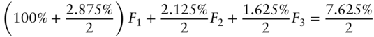
To replicate the 7.625s of 11/15/2022, Table 1.5 uses the 2.875s of 11/15/2021, the 2.125s of 05/15/2022, and the 1.625s of 11/15/2022. Number these bonds from 1 to 3, and let be the face amount of bond in the replicating portfolio. Then, the following equations express the requirement that the cash flows of the replicating portfolio equal those of the 7.625s on each of the cash flow dates. For the cash flows on November 15, 2021,

(A1.1)

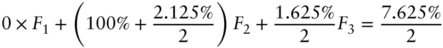
For the cash flows on May, 15, 2022,

(A1.2)

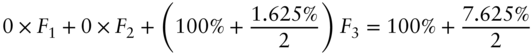
And for the cash flows on November 15, 2022,

(A1.3)

Solving equations (A1.1), (A1.2), and (A1.3) for , , and gives the replicating portfolio's face amounts reported in Table 1.5. Note that, because one bond matures on each date, these equations can be solved one‐at‐a‐time instead of simultaneously.

Replicating portfolios are easier to describe and manipulate using matrix algebra. To illustrate, equations (A1.1) through (A1.3) can be written as follows,

(A1.4)

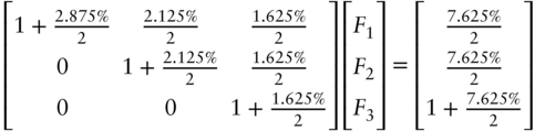
Note that each column of the leftmost matrix describes the cash flows of one of the bonds in the replicating portfolio; the elements of the vector to the right of the matrix gives the face amounts of each bond for which the equation has to be solved; and the rightmost vector gives the cash flows of the bond to be replicated. Equation (A1.4) can easily be solved.

In general, suppose that the bond to be replicated makes payments on dates. Let be the matrix of cash flows, principal plus interest, with the columns representing the bonds in the replicating portfolio and the rows the dates on which those bonds make payments. Let be the vector of face amounts in the replicating portfolio, and let be the vector of cash flows, principal plus interest, of the bond to be replicated. Then, the equation to be solved is,

(A1.5)

with solution,

(A1.6)

The only complication in constructing replicating portfolios is to ensure that the matrix does have an inverse. Essentially, any set of bonds will do so long as there is at least one bond in the replicating portfolio making a payment on each of the dates. All bonds maturing on the last date would work, for example, but all bonds maturing on the second‐to‐last date would not. In the latter case, there would be no bond in the replicating portfolio making a payment on date .

A1.2 THE EQUIVALENCE OF DISCOUNTING AND ARBITRAGE PRICING

Proposition: Pricing a bond according to either of the following methods gives the same price:

1. Derive a set of discount factors from some set of spanning bonds and price the bond in question using those discount factors.
2. Find the replicating portfolio of the bond in question using that same set of spanning bonds and calculate the price of the bond as the price of this portfolio.

Proof: Continue with the notation introduced at the end of Appendix A1.1. In addition, let be the vector of discount factors for each date and let be the vector of prices of each bond in the replicating portfolio, which is the same as the vector of prices used to compute the discount factors. Also note that a set of spanning bonds is such that the matrix has an inverse.

Generalizing the derivation of discount factors in this chapter, discount factors can be determined from the following equation,

(A1.7)

where the denotes the transpose. Then, the price of the bond according to the first method is . The price according to the second method is , where is as derived in Equation (A1.6).

Hence, the two methods give the same price if,

(A1.8)

Expanding the left‐hand side of Equation (A1.8) with (A1.7) and the right‐hand side with (A1.6),

(A1.9)

Finally, since both sides of (A1.9) are numbers, take the transpose of the left‐hand side to show that the equation is true.