
Using the right tool for the job can significantly streamline the effort involved in analyzing data. While the most obvious approach for analyzing the structured data might be to spend some extra time creating an a priori schema, importing data into it, modifying the schema because there’s something we forgot about, and then repeating the process yet a few more times, this surely wouldn’t be a very relaxing[14] thing to do. Given the very natural mapping between the document-centric nature of an email message and a JSON data structure, we’ll import our mbox data into CouchDB, a document-oriented database that provides map/reduce capabilities that are quite nice for building up indexes on the data and performing an aggregate frequency analysis that answers questions such as, “How many messages were sent by so-and-so?” or “How many messages were sent out on such-and-such a date?”
Note
A full-blown discussion about CouchDB, where it fits into the overall data storage landscape, and many of its other unique capabilities outside the ones most germane to basic analysis is outside the scope of this book. However, it should be straightforward enough to follow along with this section even if you’ve never heard of CouchDB before.
Another nice benefit of using CouchDB for the task of document analysis is that it provides an entirely REST-based interface that you can integrate into any web-based architecture, as well as trivial-to-use replication capabilities that are handy if you’d like to allow others to clone your databases (and analyses).
The remainder of this section assumes that you’re able to locate and install a CouchDB binary for your system, or compile and install it from source if that’s the way you roll. You might want to check out CouchOne, a company staffed by the creator of and primary committers for CouchDB, which provides binary downloads for most platforms and also offers some free CouchDB hosting options that you might find useful. Cloudant is another online hosting option you might want to consider.
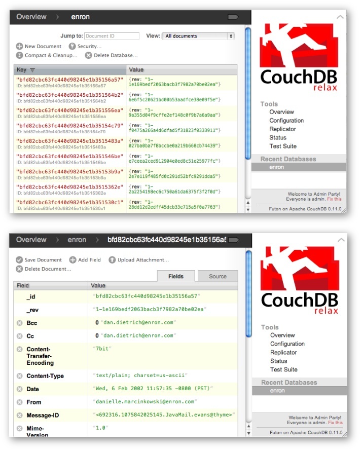
As you’re getting warmed up, you might just think of CouchDB as a key-value store where keys are arbitrary identifiers and values are JSON-based documents of your own devising. Figure 3-2 illustrates a collection of documents, as well as individual document in the collection via Futon, CouchDB’s web-based administrative interface. You can access Futon on your local installation at http://localhost:5984/_utils/.
Once CouchDB is installed, the other administrative task you’ll need
to perform is installing the Python client module couchdb via the usual easy_install couchdb approach. You can read more
about couchdb via pydoc or online at http://packages.python.org/CouchDB/. With CouchDB and a
Python client now installed, it’s time to relax and lay down some code to
ingest our JSONified mbox data—but do feel free to take a few minutes to
play around in Futon if this is your first encounter with CouchDB. If
playing things by ear doesn’t make you feel very relaxed, you should take
a brief time-out to skim the first few chapters of CouchDB: The
Definitive Guide (O’Reilly), which is available online at
http://books.couchdb.org/relax.
Running the script from Example 3-3
on the uncompressed enron.mbox file
and redirecting the output to a file yields a fairly large JSON
structure (approaching 200 MB). The script provided in Example 3-5 demonstrates how to load the data
as-is into CouchDB using couchdb-python, which you should
have already installed via easy_install couchdb. (You have
to admit that the code does look pretty relaxing compared to the
alternative gobs that would be required to load a relational schema.)
Note that it may take a couple of minutes for the script to complete if
you are using typical consumer hardware such as a laptop
computer.[15] At first, a couple of minutes might seem a bit slow, but
when you consider that the JSON structure contains more than 40,000
objects that get written out as CouchDB documents, that’s north of 300
document transactions per second, which is actually quite reasonable for
performance on an ordinary laptop. Using a performance-monitoring
utility such as top on a *nix system
or the Task Manager on Windows should reveal that one core of
your CPU is being pegged out, which would indicate maximum throughput.
During development, it’s a good idea to work with a smaller set of
documents than your full data set. You can easily slice out a dozen or
so of the JSONified Enron messages to follow along with the examples in
this chapter.
Note
Although Erlang, CouchDB’s underlying programming language, is well known for being a language that supports high concurrency, this doesn’t mean that CouchDB or any other application platform built using Erlang can necessarily keep all of the cores across all available CPUs running hot. For example, in CouchDB, write operations to a database are append-only operations that are serialized to the B-Tree on disk, and even large numbers of batch writes cannot easily be spread out across more than one core. In that regard, there is a one-to-one mapping between databases and cores for write operations. However, you could perform batch writes to multiple databases at the same time and maximize throughput across more than one core.
Example 3-5. A short script that demonstrates loading JSON data into CouchDB (mailboxes__load_json_mbox.py)
# -*- coding: utf-8 -*-

import sys
import os
import couchdb
try:
    import jsonlib2 as json
except ImportError:
    import json

JSON_MBOX = sys.argv[1]  # i.e. enron.mbox.json
DB = os.path.basename(JSON_MBOX).split('.')[0]

server = couchdb.Server('http://localhost:5984')
db = server.create(DB)
docs = json.loads(open(JSON_MBOX).read())
db.update(docs, all_or_nothing=True)
With the data loaded, it might be tempting to just sit back and relax for a while, but browsing through some of it with Futon begins to stir up some questions about the nature of who is communicating, how often, and when. Let’s put CouchDB’s map/reduce functionality to work so that we can answer some of these questions.
Note
If you’re not all that up-to-speed on map/reduce, don’t fret: learning more about it is part of what this section is all about.
In short, mapping functions take a collection of documents and map out a new key/value pair for each document, while reduction functions take a collection of documents and reduce them in some way. For example, computing the arithmetic sum of squares, f(x) = x12 + x22 + ... + xn2, could be expressed as a mapping function that squares each value, producing a one-to-one correspondence for each input value, while the reducer simply sums the output of the mappers and reduces it to a single value. This programming pattern lends itself well to trivially parallelizable problems but is certainly not a good (performant) fit for every problem. It should be clear that using CouchDB for a problem necessarily requires making some assumptions about the suitability of this computing paradigm for the task at hand.
It may not be immediately obvious, but if you take a closer look
at Figure 3-2, you’ll see that the documents you just
ingested into CouchDB are sorted by key. By default, the key is the
special _id value that’s
automatically assigned by CouchDB itself, so sort order is pretty much
meaningless at this point. In order to browse the data in Futon in a
more sensible manner, as well as performing efficient range queries,
we’ll want to perform a mapping operation to create a view that sorts by
something else. Sorting by date seems like a good idea and opens the
door to certain kinds of time-series analysis, so let’s start there and
see what happens. But first, we’ll need to make a small configuration
change so that we can write our map/reduce functions to perform this
task in Python.
CouchDB is especially intriguing in that it’s written in Erlang, a
language engineered to support super-high concurrency[16] and fault tolerance. The de facto out-of-the-box language
you use to query and transform your data via map/reduce functions is
JavaScript. Note that we could certainly opt to write map/reduce
functions in JavaScript and realize some benefits from built-in
JavaScript functions CouchDB offers—such as _sum,
_count, and _stats. But the benefit gained
from your development environment’s syntax checking/highlighting may
prove more useful and easier on the eyes than staring at JavaScript
functions wrapped up as triple-quoted string values that exist inside of
Python code. Besides, assuming you have couchdb installed, a small configuration tweak
is all that it takes to specify a Python view server so that you can
write your CouchDB code in Python. More precisely speaking, in CouchDB
parlance, the map/reduce functions are said to be view functions that reside in a special
document called a design
document .
Simply insert the following line (or a Windows compatible
equivalent) into the appropriate section of CouchDB’s local.ini configuration file, where the
couchpy executable is a view server
that will have been automatically installed along with the couchdb module. Don’t forget to restart
CouchDB after making the change:
[query_servers] python = /path/to/couchpy
Note
If you’re having trouble locating your couchpy executable on a *nix environment,
try using which couchpy in a
terminal session to find its absolute path. For Windows folks, using
the easy_install provided by ActivePython should place a
couchpy.exe
file in C:PythonXYScripts.
Watching the output when you easy_install couchdb reveals
this information.
Unless you want to write gobs and gobs of code to parse inherently
variable date strings into a standardized format, you’ll also want to
easy_install dateutil. This is a life-saving package that
standardizes most date formats, since you won’t necessarily know what
you’re up against when it comes to date stamps from a messy email
corpus. Example 3-6
demonstrates script mapping documents by their date/time stamps that you
should be able to run on the sample data we imported after configuring
your CouchDB for Python. Sample output is just a list of the documents
matching the query and is omitted for brevity.
Example 3-6. A simple mapper that uses Python to map documents by their date/time stamps (mailboxes__map_json_mbox_by_date_time.py)
# -*- coding: utf-8 -*-

import sys
import couchdb
from couchdb.design import ViewDefinition
try:
    import jsonlib2 as json
except ImportError:
    import json

DB = sys.argv[1]
START_DATE = sys.argv[2] #YYYY-MM-DD
END_DATE = sys.argv[3]   #YYYY-MM-DD

server = couchdb.Server('http://localhost:5984')
db = server[DB]

def dateTimeToDocMapper(doc):

    # Note that you need to include imports used by your mapper
    # inside the function definition

    from dateutil.parser import parse
    from datetime import datetime as dt
    if doc.get('Date'):
        # [year, month, day, hour, min, sec]
        _date = list(dt.timetuple(parse(doc['Date']))[:-3])
        yield (_date, doc)

# Specify an index to back the query. Note that the index won't be
# created until the first time the query is run

view = ViewDefinition('index', 'by_date_time', dateTimeToDocMapper,
                      language='python')
view.sync(db)

# Now query, by slicing over items sorted by date

start = [int(i) for i in START_DATE.split("-")]
end = [int(i) for i in END_DATE.split("-")]
print 'Finding docs dated from %s-%s-%s to %s-%s-%s' % tuple(start + end)

docs = []
for row in db.view('index/by_date_time', startkey=start, endkey=end):
    docs.append(db.get(row.id))
print json.dumps(docs, indent=4)
The most fundamentally important thing to understand about the
code is the role of the function dateTimeToDocMapper, a custom generator.[17] It accepts a document as a parameter and emits the same
document; however, the document is keyed by a convenient date value that
lends itself to being easily manipulated and sorted. Note that mapping
functions in CouchDB are side-effect-free; regardless of what takes
place in the mapping function or what the mapping function emits, the
document passed in as a parameter remains unaltered. In CouchDB-speak,
the dateTimeToDocMapper is a
view named “by_date_time” that’s part
of a design document called “index.”
Taking a look at Futon, you can change the combo box value in the
upper-right corner from “All documents” to “Design documents” and verify
for yourself, as shown in Figure 3-3. You
can also take a look at the pydoc for ViewDefinition for more of the same.
The first time you run the code, it should take somewhere on the order of five minutes to perform the mapping function and will keep one of your cores pegged out for most of that duration. About 80% of that time is dedicated to building the index, while the remaining time is taken up with performing the query. However, note that the index only needs to be established one time, so subsequent queries are relatively efficient, taking around 20 seconds to slice out and return approximately 2,200 documents for the date range specified, which is around 110 documents per second.
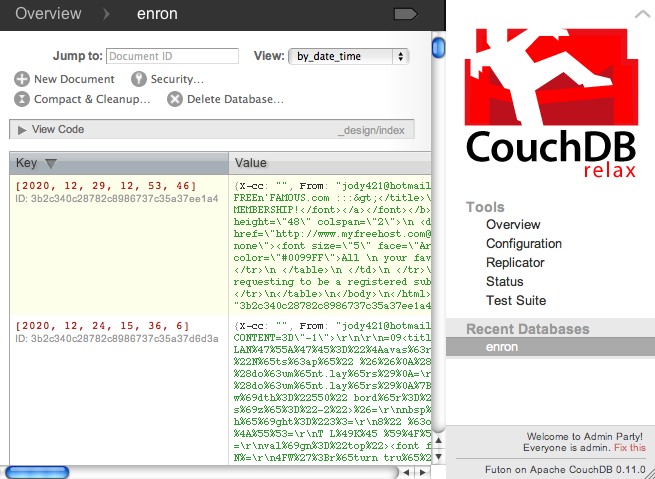
The key takeaway from this mapping function is that all of your documents are indexed by date, as can be verified in Futon by choosing the “by_date_time” index value in the “View” combo box in the upper-right corner of the screen, as shown in Figure 3-4. Although sorting documents by some criterion may not be the most interesting activity in the world, it’s a necessary step in many aggregate analytic functions, such as counting the number of documents that meet a specific criterion across an entire corpus. The next section demonstrates some basic building blocks for such analysis.
Tabulating frequencies is usually one of the first exploratory tasks you’ll want to consider when faced with a new data set, because it can tell you so much with so little effort. This section investigates a couple of ways you can use CouchDB to build frequency-based indexes.
While our by_date_time index
did a fine job of creating an index that sorts documents by date/time,
it’s not a useful index for counting the frequencies of documents
transmitted by common boundaries such as the year, month, week, etc.
While we could certainly write client code that would calculate
frequencies from a call to db.view('index/by_date_time', startkey=start,
endkey=end), it would be more efficient (and relaxing) to
let CouchDB do this work for us. All that’s needed is a trivial change
to our mapping function and the introduction of a reducing function
that’s just as trivial. The mapping function will simply emit a value
of 1 for each date/time stamp, and the reducer will count the number
of keys that are equivalent. Example 3-7 illustrates this
approach. Note that you’ll need to easy_install prettytable, a package that
produces nice tabular output, before running this example.

Note
It’s incredibly important to understand that reducing
functions only operate on values that map to the same key. A
full-blown introduction to map/reduce is beyond our scope, but
there are a number of useful resources online, including a
page in the CouchDB wiki and a
JavaScript-based interactive tool. The ins and outs of
reducers are discussed further in A Note on rereduce. None of the examples in this
chapter necessarily need to use the rereduce parameter, but to remind you
that it exists and is very important for some situations, it is
explicitly listed in all examples.
Example 3-7. Using a mapper and a reducer to count the number of messages written by date (mailboxes__count_json_mbox_by_date_time.py)
# -*- coding: utf-8 -*-

import sys
import couchdb
from couchdb.design import ViewDefinition
from prettytable import PrettyTable

DB = sys.argv[1]

server = couchdb.Server('http://localhost:5984')
db = server[DB]

def dateTimeCountMapper(doc):
    from dateutil.parser import parse
    from datetime import datetime as dt
    if doc.get('Date'):
        _date = list(dt.timetuple(parse(doc['Date']))[:-3])
        yield (_date, 1)


def summingReducer(keys, values, rereduce):
    return sum(values)


view = ViewDefinition('index', 'doc_count_by_date_time', dateTimeCountMapper,
                      reduce_fun=summingReducer, language='python')
view.sync(db)

# Print out message counts by time slice such that they're
# grouped by year, month, day

fields = ['Date', 'Count']
pt = PrettyTable(fields=fields)
[pt.set_field_align(f, 'l') for f in fields]

for row in db.view('index/doc_count_by_date_time', group_level=3):
    pt.add_row(['-'.join([str(i) for i in row.key]), row.value])

pt.printt()
Note
If you need to debug mappers or reducers written in Python,
you’ll find that printing output to the console doesn’t work. One
approach you can use that does work involves appending information
to a file. Just remember to open the file in append mode with the
'a' option: e.g., open('debug.log', 'a').
To summarize, we create a view named doc_count_by_date_time that’s stored in the
index design document; it consists
of a mapper that emits a date key for each document, and a reducer
that takes whatever input it receives and returns the sum of it. The
missing link you may be looking for is how the summingReducer function works. In this
particular example, the reducer simply computes the sum of all values
for documents that have matching keys, which amounts to counting the
number of documents that have matching keys. The way that CouchDB
reducers work in general is that they are passed corresponding lists
of keys and values, and a custom function generally performs some
aggregate operation (such as summing them up, in this case). The
rereduce parameter is a device that
makes incremental map/reduce possible by handling the case where the
results of a reducer have to themselves be reduced. No special
handling of cases involving rereducing is needed for the examples in
this chapter, but you can read more about rereducing in A Note on rereduce or online
if you anticipate needing it.
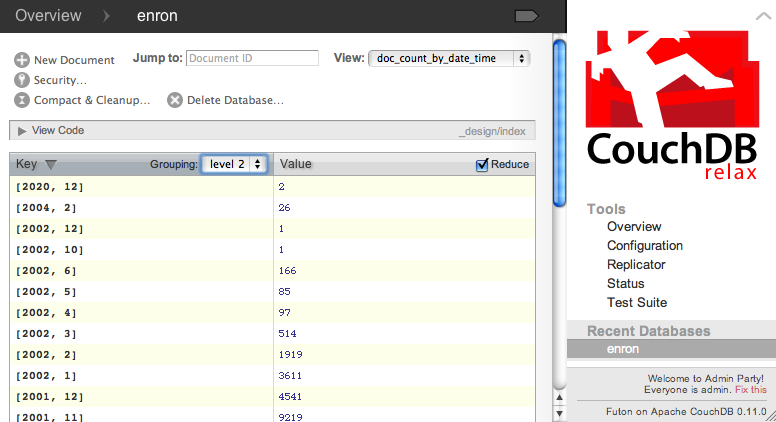
The group_level parameter is
what allows us to perform frequency analyses by various date/time
granularities associated with our key. Conceptually, CouchDB uses this
parameter to slice the first N components of the
key and automatically performs reduce operations on matching key/value
pairs. In our situation, this means calculating sums for keys that
have the first N matching components. Observe
that if the reducer were passed the full date/time key, which is
specific down to the second, we’d be querying for emails that were
sent out at exactly the same time, which probably wouldn’t be useful.
Passing in only the first component of the date/time key would tally
the number of emails sent out by year, passing in the first two
components would tally the number of emails sent out by month, etc.
The group_level keyword argument
passed to the db.view function is
how you can control what part of the key CouchDB passes into the
reducer. After running the code to compute the underlying indexes, you
can explore this functionality in Futon, as shown in Figure 3-5.
The amount of time it takes for dateTimeCountMapper to execute during the
creation of the index that backs the doc_count_by_date_time view is on par with
the previous mapping function you’ve seen, and it yields the ability
to run a number of useful queries by altering the group_level parameter. Keep in mind that
many alternative strategies, such as keying off of the number of
milliseconds since the epoch, are also possible and may be useful for
situations in which you are querying on a boundary that’s not a year,
month, week, etc. You’d have to emit the milliseconds since the epoch
as the key in your mapper and pass in keyword arguments for startkey and endkey in db.view. No reducer would necessarily be
needed.
What if you wanted to do time-based analysis that is independent
of the day, such as the number of documents that are sent out on any
given hour of the day? The grouping behavior of view queries takes
advantage of the underlying structure of the B-Tree that backs a
database, so you can’t directly
group by arbitrary items in the key in an analogous way to a Python
list slice, such as k[4:-2] or
k[4:5]. For this type of query,
you’d probably want to construct a new key with a suitable prefix,
such as [hour, minute, second].
Filtering in the client would require iterating over the entire
document collection without the added benefit of having an index
constructed for you for subsequent queries.
Other metrics, such as how many messages a given person originally authored, how many direct communications occurred between any given group of people, etc., are highly relevant statistics to consider as part of email analysis. Example 3-8 demonstrates how to calculate the number of times any two people communicated by considering the To and From fields of a message. Obviously, inclusion of Cc and Bcc fields could hold special value as well, depending on the question you are asking. The only substantive difference between this listing and Example 3-6 is that the mapping function potentially yields multiple key/value pairs. You’ll find that the pattern demonstrated can be minimally modified to compute many kinds of aggregate operations.
Example 3-8. Mapping and reducing by sender and recipient (mailboxes__count_json_mbox_by_sender_recipient.py)
# -*- coding: utf-8 -*-

import sys
import couchdb
from couchdb.design import ViewDefinition
from prettytable import PrettyTable

DB = sys.argv[1]

server = couchdb.Server('http://localhost:5984')
db = server[DB]

def senderRecipientCountMapper(doc):
    if doc.get('From') and doc.get('To'):
        for recipient in doc['To']:
            yield ([doc['From'], recipient], 1)


def summingReducer(keys, values, rereduce):
    return sum(values)


view = ViewDefinition('index', 'doc_count_by_sender_recipient',
                      senderRecipientCountMapper, reduce_fun=summingReducer,
                      language='python')
view.sync(db)

# print out a nicely formatted table
fields = ['Sender', 'Recipient', 'Count']
pt = PrettyTable(fields=fields)
[pt.set_field_align(f, 'l') for f in fields]

for row in db.view('index/doc_count_by_sender_recipient', group=True):
    pt.add_row([row.key[0], row.key[1], row.value])

pt.printt()CouchDB’s tenacious sorting of the documents in a database by key is useful for lots of situations, but there are other occasions when you’ll want to sort by value. As a case in point, it would be really useful to sort the results of Example 3-7 by frequency so that we can see the “top N” results. For small data sets, a fine option is to just perform a client-side sort yourself. Virtually every programming language has a solid implementation of the quicksort algorithm that exhibits reasonable combinatorics for the average case.[18]
For larger data sets or more niche situations, however, you may want to consider some alternatives. One approach is to transpose the reduced documents (the same ones shown in Figure 3-5, for example) and load them into another database such that the sorting can take place automatically by key. While this approach may seem a bit roundabout, it doesn’t actually require very much effort to implement, and it does have the performance benefit that operations among different databases map out to different cores if the number of documents being exported is large. Example 3-9 demonstrates this approach.
Example 3-9. Sorting documents by key by using a transpose mapper and exporting to another database (mailboxes__sort_by_value_in_another_db.py)
# -*- coding: utf-8 -*-

import sys
import couchdb
from couchdb.design import ViewDefinition
from prettytable import PrettyTable

DB = sys.argv[1]

server = couchdb.Server('http://localhost:5984')
db = server[DB]

# Query out the documents at a given group level of interest
# Group by year, month, day

docs = db.view('index/doc_count_by_date_time', group_level=3)

# Now, load the documents keyed by [year, month, day] into a new database

db_scratch = server.create(DB + '-num-per-day')
db_scratch.update(docs)


def transposeMapper(doc):
    yield (doc['value'], doc['key'])


view = ViewDefinition('index', 'num_per_day', transposeMapper, language='python')
view.sync(db_scratch)

fields = ['Date', 'Count']
pt = PrettyTable(fields=fields)
[pt.set_field_align(f, 'l') for f in fields]

for row in db_scratch.view('index/num_per_day'):
    if row.key > 10:  # display stats where more than 10 messages were sent
        pt.add_row(['-'.join([str(i) for i in row.value]), row.key])
While sorting in the client and exporting to databases are
relatively straightforward approaches that scale well for relatively
simple situations, there’s a truly industrial-strength Lucene-based
solution for comprehensive indexing of all shapes and sizes. The next
section investigates how to use couchdb-lucene for
text-based indexing—Lucene’s bread and butter—but many other
possibilities, such as sorting documents by value, indexing
geolocations, etc., are also well within reach.
Lucene is a
Java-based search engine library for high-performance full-text
indexing; its most common use is for trivially integrating keyword
search capabilities into an application. The couchdb-lucene
project is essentially a web service wrapper around some of Lucene’s
most central functionality, which enables it to index CouchDB documents.
couchdb-lucene runs as a standalone Java Virtual Machine
(JVM) process that communicates with CouchDB over HTTP, so you can run
it on a totally separate machine if you have the hardware
available.
Even a modest tutorial that scratches the surface of all that
Lucene and couchdb-lucene can do for you would be wandering
a little too far off the path. However, we will work through a brief
example that demonstrates how to get up and running with these tools in
the event that you find full-text indexing to be essential for your
tasks at hand. If full-text indexing isn’t something you necessarily
need at this time, feel free to skip this section and come back to it
later. For comparative purposes, note that it’s certainly possible to
perform text-based indexing by writing a simple mapping function that
associates keywords and documents, like the one in Example 3-10.
Example 3-10. A mapper that tokenizes documents
def tokenizingMapper(doc):
    tokens = doc.split()
    for token in tokens:
        if isInteresting(token): # Filter out stop words, etc.
            yield token, doc
However, you’ll quickly find that you need to do a lot more
homework about basic Information Retrieval (IR) concepts if you want to
establish a good scoring function to rank documents by relevance or
anything beyond basic frequency analysis. Fortunately, the benefits of
Lucene are many, and chances are good that you’ll want to use
couchdb-lucene instead of writing your own mapping function
for full-text indexing.
Note
Unlike the previous sections that opted to use the
couchdb module, this section uses httplib
to exercise CouchDB’s REST API directly and includes view functions written in
JavaScript. It seems a bit convoluted to attempt otherwise.
Binary snapshots and instructions for installing
couchdb-lucene are available at http://github.com/rnewson/couchdb-lucene. The necessary
configuration details are available in the README file, but the short of it is that, with
Java installed, you’ll need to execute couchdb-lucene’s
run script, which fires up a web server and makes a few
minor changes to CouchDB’s local.ini
configuration file so that couchdb-lucene can communicate
with CouchDB over HTTP. The key configuration changes to make are
documented in couchdb-lucene’s README. Example 3-11
demonstrates.
Note
Windows users who are interested in acquiring a service wrapper
for couchdb-lucene may want to be
advised of its potential obsolescence as of October 2010 per this
discussion thread: http://www.apacheserver.net/CouchDB-lucene-windows-service-wrapper-at1031291.htm.
Example 3-11. Configuring CouchDB to be couchdb-lucene-aware
[couchdb]
os_process_timeout=300000 ; increase the timeout from 5 seconds.

[external]
fti=/path/to/python /path/to/couchdb-lucene/tools/couchdb-external-hook.py

[httpd_db_handlers]
_fti = {couch_httpd_external, handle_external_req, <<"fti">>}
In short, we’ve increased the timeout to 5 minutes and defined a
custom behavior called fti (full text index) that invokes
functionality in a couchdb-external-hook.py script (supplied with
couchdb-lucene) whenever an _fti context for a
database is invoked. This script in turn communicates with the JVM (Java
process) running Lucene to provide full-text indexing. These details are
interesting, but you don’t necessarily have to get bogged down with them
unless that’s the way you roll.
Once couchdb-lucene is up and running, try executing
the script in Example 3-12, which
performs a default indexing operation on the Subject field as well as
the content of each document in a database. Keep in mind that with a
text-based index on the subject and content of each message, you’re
fully capable of using the normal Lucene query syntax to gain granular
control of your search. However, the default keyword capabilities are
often sufficient.
Example 3-12. Using couchdb-lucene to get full-text indexing
# -*- coding: utf-8 -*-

import sys
import httplib
from urllib import quote
import json

DB = sys.argv[1]
QUERY = sys.argv[2]

#  The body of a JavaScript-based design document we'll create

dd =
    {'fulltext': {'by_subject': {'index': '''function(doc) {
                            var ret=new Document();
                            ret.add(doc.Subject);
                            return ret
                        }'''},
     'by_content': {'index': '''function(doc) {
                            var ret=new Document();
                            for (var i=0; i < doc.parts.length; i++) {
                                ret.add(doc.parts[i].content);
                            }
                            return ret
                        }'''}}}

#  Create a design document that'll be identified as "_design/lucene"
#  The equivalent of the following in a terminal:
#  $ curl -X PUT http://localhost:5984/DB/_design/lucene -d @dd.json

try:
    conn = httplib.HTTPConnection('localhost', 5984)
    conn.request('PUT', '/%s/_design/lucene' % (DB, ), json.dumps(dd))
    response = conn.getresponse()
finally:
    conn.close()

if response.status != 201:  #  Created
    print 'Unable to create design document: %s %s' % (response.status,
            response.reason)
    sys.exit()

#  Querying the design document is nearly the same as usual except that you reference
#  couchdb-lucene's _fti HTTP handler
#  $ curl http://localhost:5984/DB/_fti/_design/lucene/by_subject?q=QUERY

try:
    conn.request('GET', '/%s/_fti/_design/lucene/by_subject?q=%s' % (DB,
                 quote(QUERY)))
    response = conn.getresponse()
    if response.status == 200:
        response_body = json.loads(response.read())
        print json.dumps(response_body, indent=4)
    else:
        print 'An error occurred fetching the response: %s %s'
            % (response.status, response.reason)
finally:
    conn.close()
You’ll certainly want to reference the online
couchdb-lucene documentation for
the full scoop, but the gist is that you create a specially formatted
design document that contains a fulltext field, which houses the name of an
index and a JavaScript-based indexing function. That indexing function
returns a Document object containing fields that Lucene
should index. Note that the Document
object is defined by couchdb-lucene (not CouchDB) when your
index is built. A sample query result for the infamous word
“raptor”[19] returns the response shown in Example 3-13. Notice that you’d use the
id values to look up documents for
display for further analysis from CouchDB directly.
Example 3-13. Sample query results for “raptor” on the Enron data set
/* Sample query results for
http://localhost:5984/enron/_fti/_design/lucene/by_content?q=raptor */

{ "etag" : "11b7c665b2d78be0",
  "fetch_duration" : 2,
  "limit" : 25,
  "q" : "default:raptor",
  "rows" : [ { "id" : "3b2c340c28782c8986737c35a355d0eb",
        "score" : 1.4469228982925415
      },
      { "id" : "3b2c340c28782c8986737c35a3542677",
        "score" : 1.3901585340499878
      },
      { "id" : "3b2c340c28782c8986737c35a357c6ae",
        "score" : 1.375900149345398
      },

      /* ... output truncated ... */

      { "id" : "2f84530cb39668ab3cdab83302e56d65",
        "score" : 0.8107569217681885
      }
    ],
  "search_duration" : 0,
  "skip" : 0,
  "total_rows" : 72
  }
Full details about the response are available in the
documentation, but the most interesting part is the collection of rows
containing document ID values that you can use to access the documents
in CouchDB. In terms of data flow, you should note that you haven’t
directly interacted with couchdb-lucene at all, per se;
you’ve simply defined a specially crafted design document and issued a
query to CouchDB, which knows what to do based on the presence of
fulltext and _fti in the design document and query,
respectively. A discussion of Lucene’s specific techniques for scoring
documents is outside the scope of this book, but you can read more about
it in its scoring
documentation and, more specifically, in the Similarity
class. It’s unlikely that you can customize Lucene’s scoring properties
(should you need to do so) without modifying Lucene’s source code, but
you should be able to influence scoring by passing through parameters
such as “boost”
via the various API parameters that couchdb-lucene exposes,
as opposed to hacking the source code.
If you’re at all familiar with the term “raptor” as it relates to the Enron story, you might find the first few lines of the most highly ranked message in the search results helpful as context:
The quarterly valuations for the assets hedged in the Raptor structure were valued through the normal quarterly revaluation process. The business units, RAC and Arthur Andersen all signed off on the initial valuations for the assets hedged in Raptor. All the investments in Raptor were on the MPR and were monitored by the business units, and we prepared the Raptor position report based upon this information….
If you’re swimming in a collection of thousands of messages and aren’t sure where to start looking, that simple keyword search certainly guided you to a good starting point. The subject of the message just quoted is “RE: Raptor Debris.” Wouldn’t it be interesting to know who else was in on that discussion thread and other threads about Raptor? Not so coincidentally, that’s the topic of the next section.
[14] CouchDB folks tend to overuse the word “relax,” and this discussion follows suit in an effort to be as authentic as possible.
[15] For the purposes of comparison, it takes about two minutes to execute Example 3-5 on a MacBook Pro 2.8GHz Core 2 Duo with CouchDB 0.11.0 installed using stock settings.
[16] Generally speaking, the characteristic of having “high concurrency” means that multiple operations can be run at the same time (concurrently) across multiple cores on a microprocessor, yielding maximum CPU throughput.
[17] Loosely speaking, a generator is a function that returns an iterator. See http://docs.python.org/tutorial/classes.html.
[18] On average, quicksort makes n*lg(n) comparisons
to sort a collection in the worst case, which is about the best you
can do without knowing any prior information to tailor the algorithm
to the data.
[19] In the context of Enron, Raptors were financial devices used to hide losses. Enron used them to keep hundreds of millions in debt out of the accounting books.