
Although rigorous approaches to natural language processing (NLP) that include such things as sentence segmentation, tokenization, word chunking, and entity detection are necessary in order to achieve the deepest possible understanding of textual data, it’s helpful to first introduce some fundamentals from Information Retrieval theory. The remainder of this chapter introduces some of its more foundational aspects, including TF-IDF, the cosine similarity metric, and some of the theory behind collocation detection. Chapter 8 provides a deeper discussion of NLP.
Note
If you want to dig deeper into IR theory, the full text of Introduction to Information Retrieval is available online and provides more information than you could ever want to know about the field.
Information retrieval is an extensive field with many specialties.
This discussion narrows in on TF-IDF, one of the most fundamental
techniques for retrieving relevant documents from a corpus. TF-IDF
stands for term frequency-inverse document
frequency and can be used to query a corpus by calculating
normalized scores that express the relative importance of terms in the
documents. Mathematically, TF-IDF is expressed as the product of the
term frequency and the inverse document frequency, tf_idf =
tf*idf, where the term tf
represents the importance of a term in a specific document, and idf represents the importance of a term
relative to the entire corpus. Multiplying these terms together produces
a score that accounts for both factors and has been an integral part of
every major search engine at some point in its existence. To get a more
intuitive idea of how TF-IDF works, let’s walk through each of the
calculations involved in computing the overall score.
For simplicity in illustration, suppose you have a corpus containing three sample documents and terms are calculated by simply breaking on whitespace, as illustrated in Example 7-3.
Example 7-3. Sample data structures used in illustrations throughout this chapter
corpus = {
        'a' : "Mr. Green killed Colonel Mustard in the study with the candlestick.
               Mr. Green is not a very nice fellow.",
        'b' : "Professor Plumb has a green plant in his study.",
        'c' : "Miss Scarlett watered Professor Plumb's green plant while he was away
               from his office last week."
}

terms = {
        'a' : [ i.lower() for i in corpus['a'].split() ],
        'b' : [ i.lower() for i in corpus['b'].split() ],
        'c' : [ i.lower() for i in corpus['c'].split() ]
        }
A term’s frequency could simply be represented as the number of
times it occurs in the text, but it is more commonly the case that it is
normalized by taking into account the total number of terms in the text,
so that the overall score accounts for document length relative to a
term’s frequency. For example, the term “green” (once normalized to
lowercase) occurs twice in
corpus['a'] and only once in corpus['b'], so
corpus['a'] would produce a higher score if frequency were
the only scoring criterion. However, if you normalize for document
length, corpus['b'] would have a slightly higher term
frequency score for “green” (1/9) than corpus['a'] (2/19),
because corpus['b'] is shorter than
corpus['a']—even though “green” occurs more frequently in
corpus['a']. Thus, a common technique for scoring a
compound query such as “Mr. Green” is to sum the term frequency scores
for each of the query terms in each document, and return the documents
ranked by the summed term frequency score.
The previous paragraph is actually not as confusing as it sounds; for example, querying our sample corpus for “Mr. Green” would return the normalized scores reported in Table 7-1 for each document.
Table 7-1. Sample term frequency scores for “Mr. Green”
| Document | tf(Mr.) | tf(Green) | Sum |
|---|---|---|---|
| corpus['a'] | 2/19 | 2/19 | 4/19 (0.2105) |
| corpus['b'] | 0 | 1/9 | 1/9 (0.1111) |
| corpus['c'] | 0 | 1/16 | 1/16 (0.0625) |
For this contrived example, a cumulative term frequency scoring
scheme works out and returns corpus['a'] (the document that
we’d expect it to return), since corpus['a'] is the only one that contains
the compound token “Mr. Green”. However, a number of problems could have
emerged because the term frequency scoring model looks at each document
as an unordered collection of words. For example, queries for “Green
Mr.” or “Green Mr. Foo” would have returned the exact same scores as the
query for “Mr. Green”, even though neither of those compound tokens
appear in the sample sentences. Additionally, there are a number of
scenarios that we could easily contrive to illustrate fairly poor
results from the term frequency ranking technique by exploiting the fact
that trailing punctuation is not properly handled, and the context
around tokens of interest is not taken into account by the
calculations.
Considering term frequency alone turns out to be a common problem
when scoring on a document-by-document basis because it doesn’t account
for very frequent words that are common across many documents. Meaning,
all terms are weighted equally regardless of their actual importance.
For example, “the green plant” contains the stopword “the”, which skews
overall term frequency scores in favor of corpus['a']
because “the” appears twice in that document, as does “green”. In
contrast, in corpus['c'] “green” and “plant” each appear
only once.
Consequently, the scores would break down as shown in Table 7-2, with corpus['a'] ranked as more
relevant than corpus['c'] even though intuition might lead
you to believe that ideal query results probably shouldn’t have turned
out that way. (Fortunately, however, corpus['b'] still
ranks highest.)
Table 7-2. Sample term frequency scores for “the green plant”
| Document | tf(the) | tf(green) | tf(plant) | Sum |
|---|---|---|---|---|
| corpus['a'] | 2/19 | 2/19 | 0 | 4/19 (0.2105) |
| corpus['b'] | 0 | 1/9 | 1/9 | 2/9 (0.2222) |
| corpus['c'] | 0 | 1/16 | 1/16 | 1/8 (0.125) |
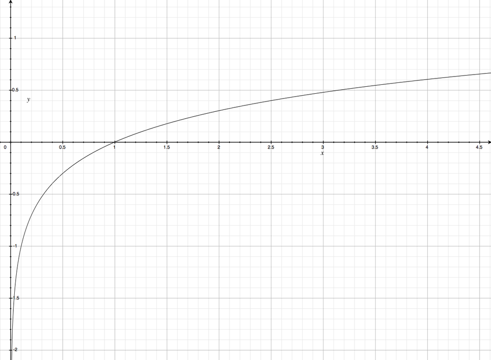
Toolkits such as NLTK provide lists of stopwords that can be used to filter out terms such as “the”, “a”, “and”, etc., but keep in mind that there may be terms that evade even the best stopword lists and yet still are quite common to specialized domains. The inverse document frequency metric is a calculation that provides a generic normalization metric for a corpus, and accounts for the appearance of common terms across a set of documents by taking into consideration the total number of documents in which a query term ever appears. The intuition behind this metric is that it produces a higher value if a term is somewhat uncommon across the corpus than if it is very common, which helps to account for the problem with stopwords we just investigated. For example, a query for “green” in the corpus of sample documents should return a lower inverse document frequency score than “candlestick”, because “green” appears in every document while “candlestick” appears in only one. Mathematically, the only nuance of interest for the inverse document frequency calculation is that a logarithm is used to squash the result into a compressed range (as shown in Figure 7-3) since its usual application is in multiplying it against term frequency as a scaling factor.
At this point, we’ve come full circle and devised a way to compute
a score for a multiterm query that accounts for the frequency of terms
appearing in a document, the length of the document in which any
particular term appears, and the overall uniqueness of the terms across
documents in the entire corpus. In other words, tf-idf = tf*idf. Example 7-4 is a naive implementation of this discussion
that should help solidify the concepts described. Take a moment to
review it, and then we’ll discuss a few sample queries.
Example 7-4. Running TF-IDF on sample data (plus__tf_idf.py)
# -*- coding: utf-8 -*-

import sys
from math import log

QUERY_TERMS = sys.argv[1:]


def tf(term, doc, normalize=True):
    doc = doc.lower().split()
    if normalize:
        return doc.count(term.lower()) / float(len(doc))
    else:
        return doc.count(term.lower()) / 1.0


def idf(term, corpus):
    num_texts_with_term = len([True for text in corpus if term.lower()
                              in text.lower().split()])

    # tf-idf calc involves multiplying against a tf value less than 0, so it's important
    # to return a value greater than 1 for consistent scoring. (Multiplying two values
    # less than 1 returns a value less than each of them)

    try:
        return 1.0 + log(float(len(corpus)) / num_texts_with_term)
    except ZeroDivisionError:
        return 1.0


def tf_idf(term, doc, corpus):
    return tf(term, doc) * idf(term, corpus)


corpus =
    {'a': 'Mr. Green killed Colonel Mustard in the study with the candlestick.
Mr. Green is not a very nice fellow.',
     'b': 'Professor Plumb has a green plant in his study.',
     'c': "Miss Scarlett watered Professor Plumb's green plant while he was away
from his office last week."}

# Score queries by calculating cumulative tf_idf score for each term in query

query_scores = {'a': 0, 'b': 0, 'c': 0}
for term in [t.lower() for t in QUERY_TERMS]:
    for doc in sorted(corpus):
        print 'TF(%s): %s' % (doc, term), tf(term, corpus[doc])
    print 'IDF: %s' % (term, ), idf(term, corpus.values())
    print

    for doc in sorted(corpus):
        score = tf_idf(term, corpus[doc], corpus.values())
        print 'TF-IDF(%s): %s' % (doc, term), score
        query_scores[doc] += score
    print

print "Overall TF-IDF scores for query '%s'" % (' '.join(QUERY_TERMS), )
for (doc, score) in sorted(query_scores.items()):
    print doc, score
Although we’re working on a trivially small scale, the calculations involved work the same for larger data sets. Table 7-3 is a consolidated adaptation of the program’s output for three sample queries that involve four distinct terms:
“green”
“Mr. Green”
“the green plant”
Even though the IDF calculations for terms are for the entire corpus, they are displayed on a per-document basis so that you can easily verify TF-IDF scores by skimming a single row and multiplying two numbers. Again, it’s worth taking a few minutes to understand the data in the table so that you have a good feel for the way the calculations work. It’s remarkable just how powerful TF-IDF is, given that it doesn’t account for the proximity or ordering of words in a document.
Table 7-3. Calculations involved in TF-IDF sample queries, as computed by Example 7-4
| Document | tf(mr.) | tf(green) | tf(the) | tf(plant) |
|---|---|---|---|---|
| corpus['a'] | 0.1053 | 0.1053 | 1.1053 | 0 |
| corpus['b'] | 0 | 0.1111 | 0 | 0.1111 |
| corpus['c'] | 0 | 0.0625 | 0 | 0.0625 |
| idf(mr.) | idf(green) | idf(the) | idf(plant) | |
|---|---|---|---|---|
| corpus['a'] | 2.0986 | 1.0 | 2.099 | 1.4055 |
| corpus['b'] | 2.0986 | 1.0 | 2.099 | 1.4055 |
| corpus['c'] | 2.0986 | 1.0 | 2.099 | 1.4055 |
| tf-idf(mr.) | tf-idf(green) | tf-idf(the) | tf-idf(plant) | |
|---|---|---|---|---|
| corpus['a'] | 0.2209 | 0.1053 | 0.2209 | 0 |
| corpus['b'] | 0 | 0.1111 | 0 | 0.1562 |
| corpus['c'] | 0 | 0.0625 | 0 | 0.0878 |
The same results for each query are shown in Table 7-4, with the TF-IDF values summed on a per-document basis.
Table 7-4. Summed TF-IDF values for sample queries as computed by Example 7-4
| Query | corpus['a'] | corpus['b'] | corpus['c'] |
|---|---|---|---|
| green | 0.1053 | 0.1111 | 0.0625 |
| Mr. Green | 0.2209 + 0.1053 = 0.3262 | 0 + 0.1111 = 0.1111 | 0 + 0.0625 = 0.0625 |
| the green plant | 0.2209 + 0.1053 + 0 = 0.3262 | 0 + 0.1111 + 0.1562 = 0.2673 | 0 + 0.0625 + 0.0878 = 0.1503 |
From a qualitative standpoint, the query results seem reasonable.
The corpus['b'] document is the winner
for the query “green”, with corpus['a'] just a hair behind.
In this case, the deciding factor was the length of
corpus['b'] being much smaller than
corpus['a']: the normalized TF score tipped in favor of
corpus['b'] for its one occurrence of “green”, even though
“Green” appeared in corpus['a'] two times. Since “green”
appears in all three documents, the net effect of the IDF term in the
calculations was a wash. Do note, however, that if we had returned 0.0
instead of 1.0 for IDF calculations, as is done in some implementations,
the TF-IDF scores for “green” would have been 0.0 for all three
documents. Depending on the particular situation, it may be better to
return 0.0 for the IDF scores rather than 1.0. For example, if you had
100,000 documents and “green” appeared in all of them, you’d almost
certainly consider it to be a stopword and want to remove its effects in
a query entirely.
Note
A very worthwhile exercise to consider is why
corpus['a'] scored highest for “the green plant” as
opposed to corpus['b'], which at first blush, might
have seemed a little more obvious.
A finer point to observe is that the sample implementation
provided in Example 7-4 adjusts the IDF score by
adding a value of 1.0 to the logarithm calculation, for the purposes of
illustration and because we’re dealing with a trivial document set.
Without the 1.0 adjustment in the calculation, it would be possible to
have the idf function return values
that are less than 1.0, which would result in two fractions being
multiplied in the TF-IDF calculation. Since multiplying two fractions
together results in a value smaller than either of them, this turns out
to be an easily overlooked edge case in the TF-IDF calculation. Recall
that the intuition behind the TF-IDF calculation is that we’d like to be
able to multiply two terms in a way that consistently produces larger
TF-IDF scores for more-relevant queries than for less-relevant
queries.
Let’s apply TF-IDF to the Google+ data we collected earlier and see how it works out as a tool for querying the data. NLTK provides some abstractions that we can use instead of rolling our own, so there’s actually very little to do now that you understand the underlying theory. The listing in Example 7-5 assumes you saved the Google+ data as a JSON file, and it allows you to pass in multiple query terms that are used to score the documents by relevance.
Example 7-5. Querying Google+ data with TF-IDF (plus__tf_idf_nltk.py)
# -*- coding: utf-8 -*-

import sys
import json
import nltk

# Load in unstructured data from wherever you've saved it

DATA = sys.argv[1]
data = json.loads(open(DATA).read())

QUERY_TERMS = sys.argv[2:]

activities = [activity['object']['content'].lower().split()
              for activity in data
                if activity['object']['content'] != ""]

# Provides tf/idf/tf_idf abstractions

tc = nltk.TextCollection(activities)

relevant_activities = []

for idx in range(len(activities)):
    score = 0
    for term in [t.lower() for t in QUERY_TERMS]:
        score += tc.tf_idf(term, activities[idx])
    if score > 0:
        relevant_activities.append({'score': score, 'title': data[idx]['title'],
                              'url': data[idx]['url']})

# Sort by score and display results

relevant_activities = sorted(relevant_activities, key=lambda p: p['score'], reverse=True)
for activity in relevant_activities:
    print activity['title']
    print '	Link: %s' % (activity['url'], )
    print '	Score: %s' % (activity['score'], )
Sample query results for “SOPA”, a controversial piece of proposed legislation, on Tim O’Reilly’s Google+ data are shown in Example 7-6.
Example 7-6. Sample results from Example 7-5
I think the key point of this piece by +Mike Loukides, that PIPA and SOPA provide a
"right of ext...
	Link: https://plus.google.com/107033731246200681024/posts/ULi4RYpvQGT
	Score: 0.0805961208217
Learn to Be a Better Activist During the SOPA Blackouts +Clay Johnson has put together
an awesome...
	Link: https://plus.google.com/107033731246200681024/posts/hrC5aj7gS6v
	Score: 0.0255051015259
SOPA and PIPA are bad industrial policy There are many arguments against SOPA and PIPA
that are b...
	Link: https://plus.google.com/107033731246200681024/posts/LZs8TekXK2T
	Score: 0.0227351539694
Further thoughts on SOPA, and why Congress shouldn't listen to lobbyists Colleen Taylor
of GigaOM...
	Link: https://plus.google.com/107033731246200681024/posts/5Xd3VjFR8gx
	Score: 0.0112879721039
Given a search term, being able to narrow in on three Google+
content items ranked by relevance is of tremendous benefit when
analyzing unstructured text data. Try out some other queries and
qualitatively review the results to see for yourself how well the TF-IDF
metric works, keeping in mind that the absolute values of the scores
aren’t really important—it’s the
ability to find and sort documents by relevance that matters. Then,
begin to ponder the gazillion ways that you could tune or augment this
metric to be even more effective. (After all, every data hacker has to
complete this exercise at some point in life.) One obvious improvement
that’s left as an exercise for the reader is to stem verbs so that
variations in tense, grammatical role, etc., resolve to the same stem
and can be more accurately accounted for in similarity calculations. The
nltk.stem module provides easy-to-use implementations for
several common stemming algorithms.