
“For every simple problem, there is a complex solution that is wrong.”
—Anonymous
The term “two-phase flow” covers an extremely broad range of situations, and it is possible to address only a small portion of this spectrum in one book, let alone one chapter. A “two-phase flow” includes any combination of two of the three phases: solid, liquid, and gas, that is, solid–liquid, gas–liquid, solid–gas, or liquid–liquid. Also, if both phases are fluids (combinations of liquid and/or gas), one of the phases may be continuous and the other distributed (e.g., gas in liquid or liquid in gas). Furthermore, the mass ratio of the two phases may be fixed or variable throughout the system. Examples of the former are nonvolatile liquids with entrained solids or noncondensable gases, whereas examples of the latter are flashing liquids, soluble solids in liquids, and partly miscible liquids in liquids. Additional situations are encountered in boilers and condensers in which phase change occurs. One can also encounter three phases like in slurry reactors, three phase fluidized beds, etc.
In addition, in pipe flows, the two phases may be highly mixed and uniformly distributed over the cross section (i.e., “homogeneous”) or they may be “separated” into two distinct regions, and the conditions under which these states prevail are different for horizontal than for vertical flow and depend upon the type of system, for example, gas–liquid, gas–solid, solid–liquid, liquid–liquid, or even gas–liquid–solid. For uniformly distributed homogeneous flows, the fluid can be described as a “pseudo-single-phase fluid,” with properties of the mixture being average values of the two phases over the flow cross section. Such flows can be described as “1-D,” as opposed to “separated” or heterogeneous, in which the phase distribution varies over the cross section.
In this chapter, we will focus on two-phase flows in pipes, which includes the transport of solids as slurries and suspensions in a continuous liquid phase, pneumatic transport of solid particles in a continuous gas phase, and mixtures of gas or vapor with liquids in which either phase may be continuous. Although it may appear that only one additional “variable” is added to the single-phase problems previously considered, the complexity of two-phase flows is indeed greater by orders of magnitude. It is emphasized that this is only an introduction and literally thousands of articles abound in the literature on various aspects of two-phase flows. It should also be realized that if these problems were simple or straightforward, the number of papers required to describe them would be orders of magnitude smaller. Detailed treatments can also be found in several excellent books including Wallis (1969), Govier and Aziz (1983), Hetsroni (1982), Levy (1999) and Michaelides et al. (2016).
Before proceeding, it is appropriate to define the terminology for the various flow rates, velocities, and concentrations for two-phase flows. There is a bewildering variety of notation in the literature relative to two-phase flow, and we will attempt to use a notation that is consistent with the following definitions for solid–liquid, solid–gas, and liquid–gas systems.
The subscripts m, L, S, and G represent the local two-phase mixture, liquid phase, solid phase, and gas phase, respectively. The definitions in the following text are given in terms of solid–liquid (S-L) mixtures, where the solid is the more dense distributed phase and the liquid the less dense continuous phase. The same definitions can be applied to gas–liquid (G-L) flows in which the gas is the continuous phase and the liquid the distributed phase if the subscript S is replaced by L (the more dense distributed phase) and L by G (the less dense continuous phase). The symbol φ is used for the volume fraction of the distributed (dense) phase and ε is the volume fraction of the continuous phase (obviously φ = 1 – ε). (For gas–liquid flows, the volume fraction of gas is often denoted by α (i.e., α = ε).
An important distinction is made between (φ, ε) and (φm, εm). The former (φ, ε) refers to the overall flow-average (equilibrium) values entering the pipe, that is,
(16.1) |
whereas the latter (φm, εm) refer to the local values at a given position in the pipe. These are different (φm ≠ φ, εm ≠ ε) when the local velocities of the two phases are not the same (i.e., slip is significant), as will be shown later.
Mass flow rate (ṁ) and volume flow rate (Q):
(16.2) |
Mass flux (G):
(16.3) |
where A is the conduit cross-sectional area.
Volume flux:
(16.4) |
Phase velocity:
(16.5) |
Relative (slip) velocity and slip ratio:
(16.6) |
Note that the total volume flux (Jm) of the mixture is the same as the superficial velocity, Vm (the volumetric flow rate divided by the total flow area). However, the local velocity of each phase (Vi) is greater than the volume flux of that phase (Ji), since each phase occupies only a fraction of the total flow area. This is akin to the interstitial velocity versus the superficial velocity in the context of flow in packed beds and porous media (Chapter 14). The volume flux of each phase is the total volume flow rate of that phase divided by the total flow area.
The relative slip velocity (or slip ratio) is an extremely important variable. This occurs primarily when the distributed phase density is greater than that of the continuous phase and the heavier distributed phase tends to lag behind the lighter phase for various reasons (explained later). The resulting relative velocity (slip) between the phases determines the drag exerted by the continuous (lighter) phase on the distributed (heavier) phase. One consequence of slip (as shown later) is that the in situ concentration or “holdup” of the more dense phase within the pipe (φm) is greater than that entering or leaving the pipe, since its residence time is longer than that of the continuous phase. Consequently, the concentrations and local phase velocities within a pipe under slip conditions depend upon the properties and degree of interaction of the phases and cannot be determined solely from the knowledge of the entering and leaving concentrations and flow rates. Slip can only be determined indirectly by measurement of some local flow property within the pipe, such as the holdup, concentration profiles, local phase velocity, or the local mixture density.
For example, for transport of solid particles by a liquid, if φ is the solids volume fraction entering the pipe at velocity V and φm is the local volume fraction in the pipe where the solid velocity is VS, a component balance shows
(16.7) |
Substituting these expressions in the definition of the slip velocity, Equation 16.6, and dividing by the inlet velocity (V) to make the results dimensionless gives
(16.8) |
This can be solved for φm in terms of and φ:
(16.9) |
As an example, if the entering solids fraction φ is 0.4, the corresponding values of the local solids fraction φm for relative slip velocities of 0.01, 0.1, and 0.5 are 0.403, 0.424, and 0.525, respectively. There are many “theoretical” expressions for predicting the slip velocity, but practical applications depend on experimental observations and correlations (which will be presented later). In gas–liquid or gas–solid flows, φm will vary along the pipe since the gas expands as the pressure drops and speeds up as it expands, which increases the slip. This, in turn, increases the holdup of the denser phase (more on slip and holdup later).
The mass fraction (x) of the less dense phase (which, for gas–liquid flows, is called the quality) is ,so that the mass flow ratio can be written as
(16.10) |
This can be rearranged to give the less dense phase volume fraction (εm or α) in terms of the mass fraction and slip ratio:
(16.11) |
The local density of the mixture is given by
(16.12) |
which depends on the slip ratio S through Equation 16.11. The corresponding expression for the local in-situ holdup of the denser phase is
(16.13) |
Note that both the local mixture density and holdup increase as the slip ratio (S) increases. The “no-slip” (S = 1) density or volume fraction is identical to the equilibrium value entering (or leaving) the pipe.
III. FLUID–SOLID TWO-PHASE PIPE FLOWS
The conveying of solids by a fluid in a pipe involves a wide range of flow conditions and phase distributions, depending on the density, viscosity, and velocity of the fluid; the density, size, shape, and concentration of the solid particles; or the orientation of the pipe (vertical, horizontal, or inclined). The flow regime can vary from essentially uniformly distributed solids in a “pseudohomogeneous” (symmetric) flow regime for sufficiently small and/or light particles and/or a very high mixture velocity, to an almost completely segregated or stratified (asymmetric) transport of a bed of particles along the pipe wall. The demarcation between the “homogeneous” and “heterogeneous” flow regimes depends in a complex manner on the size and density of the solids, the fluid density and viscosity, the velocity of the mixture, and the volume fraction of solids. Furthermore, the transition from one flow regime to another is far from being sharp. Figure 16.1 illustrates the approximate effect of particle size, density, and solids loading on these regimes.
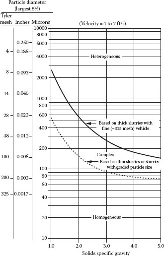
FIGURE 16.1 Approximate slurry flow regimes. (From Aude, T.C. et al., Slurry piping systems: Trends, design methods, guidelines, Chem. Eng., 74, June 28, 1971.)
Either a liquid or a gas can be used as the carrier fluid, depending on the size and properties of the particles. However, there are important differences between hydraulic (liquid) and pneumatic (gas) transport. For example, in hydraulic (liquid) transport, fluid–particle and particle–particle interactions dominate over the particle–wall interactions, whereas in gas (pneumatic) transport, the particle–particle and particle–wall interactions tend to dominate over the fluid–particle interactions. A typical “practical” approach, which gives reasonable results for a wide variety of flow conditions in both cases, is to determine the “fluid only” pressure drop and then apply a correction to account for the effect of the particles from the fluid–particle, particle–particle, and/or particle–wall interactions. A great number of studies have been devoted to this subject, and summaries of much of this work have been given by Darby (1986), Govier and Aziz (1983), Klinzing et al. (2010), Molerus (1993), Wasp et al. (1977), Brown and Heywood (1991), Shook and Roco (1991) and Wilson et al. (2008). This approach will be described later.
If the solid particles are very small (e.g., typically less than 100 μm), and/or not greatly denser than the fluid, and/or the flow is highly turbulent, the mixture may behave as a uniform suspension with essentially continuous properties with no slip between the two phases. In this case, the mixture can be described as a “pseudo-single-phase” uniform fluid, and the effect of the presence of the particles can be accounted for by appropriate modification of the fluid properties (density and viscosity). For relatively dilute suspensions (e.g., 5% by volume or less), the mixture will behave as a Newtonian fluid with a viscosity given by the Einstein equation:
(16.14) |
where
μL is the viscosity of the suspending (continuous) Newtonian fluid
φ = (1 – ε) is the volume fraction of solids
and the density of the mixture is given by
(16.15) |
For greater concentrations of fine particles, the suspension is more likely to be non-Newtonian, in which case the viscous properties can probably be adequately described by the power law or Bingham plastic (preferred) models. The pressure drop–flow relationship for pipe flow under these conditions can be determined by the methods presented in Chapters 6 and 7.
B. HETEROGENEOUS LIQUID–SOLID FLOWS
Figure 16.2 shows how the pressure gradient and flow regimes in a horizontal pipe depend upon the velocity for a typical heterogeneous suspension. It is seen that the pressure gradient exhibits a minimum at the “minimum deposit velocity,” which is the velocity at which a significant amount of solids begin to settle in the pipe. Under these conditions, most of the particles are transported in the form of a sliding or moving bed along the pipe wall. This not only leads to a high pressure gradient but it can also cause severe erosion and wear of the pipe. A variety of correlations have been proposed in the literature for the prediction of the minimum deposit velocity, one of the more useful being that of Hanks (1980):
(16.16) |
where s = ρS/ρL. At velocities below this value, the solids settle out and form a bed along the bottom of the pipe. This bed can build up and eventually plug the pipe if the velocity is too low, or it can be swept along the pipe wall if the velocity is near the minimum deposit velocity. Above the minimum deposit velocity, the particles are suspended but are not uniformly distributed (“symmetric”) until the turbulent mixing is high enough to overcome the settling forces and/or can resuspend at least some of the settled particles. One criterion for a nonsettling suspension has been given by Wasp et al. (1977):
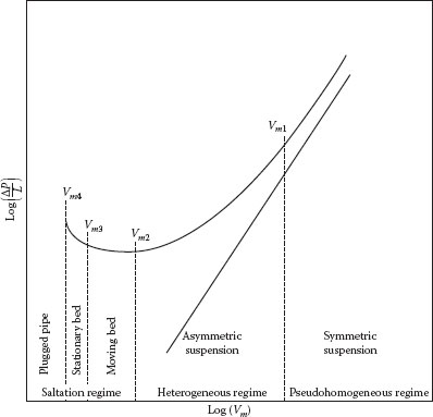
FIGURE 16.2 Pressure gradient and flow regimes for slurry flow in a horizontal pipe.
(16.17) |
where
Vt is the particle terminal velocity in a quiescent fluid
V* is the friction velocity, defined as
(16.18) |
For heterogeneous flow, one approach to determining the pressure drop in a pipe is to compute separately the contributions of the fluid and the solids at the same velocity:
(16.19) |
where
ΔPL is the “fluid only” pressure drop
ΔPS is an additional pressure drop due to the presence of the solids
For uniform sized particles in a Newtonian liquid, ΔPL is determined as for any Newtonian fluid in a pipe at the same flow rate as that of the mixture. For a broad particle size distribution, the suspension may behave more like a heterogeneous suspension of the larger particles in a carrier vehicle composed of a homogeneous suspension of the finer particles. In this case, the homogeneous carrier will likely be non-Newtonian, and the methods given in Chapter 6 for such fluids should be used to determine ΔPL.
The procedure for determining ΔPS that will be presented here is that of Molerus (1993). The basis of the method is a consideration of the extra energy dissipated in the flow as a result of the fluid–particle interaction. This is characterized by the particle terminal settling velocity in an infinite fluid in terms of the drag coefficient, Cd:
(16.20) |
where s = ρS/ρL. Molerus (1993) applied dimensional analysis to the variables in this system, along with energy dissipation considerations, to arrive at the following dimensionless groups:
(16.21) |
(16.22) |
(16.23) |
where
V is the overall average velocity in the pipe
Vr = VL – VS is the relative (“slip”) velocity between the fluid and the solid
Vt is the terminal velocity of the solid particle
d is the particle diameter
D is the tube diameter
NFrp is the particle Froude number
NFrt is the tube Froude number
The slip velocity is the key parameter in the mechanism of transport and energy dissipation because the drag force exerted by the fluid on the particle depends on the relative velocity between the fluid and particles. That is, the fluid must move faster than the particles in order to carry them along the pipe. The particle terminal velocity is related to the particle drag coefficient and Reynolds number, as discussed in Chapter 12 (e.g., unknown velocity), for either a Newtonian or non-Newtonian carrier medium.
Molerus (1993) developed a “state diagram” that shows a correlation between these dimensionless groups based on an extremely wide range of data covering 25 < D < 315 mm, 12 < d < 5200 μm, and 1270 < ρS < 5250 kg/m3 for both hydraulic and pneumatic transport. This state diagram is shown in Figure 16.3 in the following form:
(16.24) |
where is the dimensionless “single-particle” slip velocity as determined from the diagram,
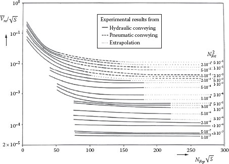
FIGURE 16.3 State diagram for suspension transport. (From Molerus, O., Principles of Flow in Disperse Systems, Chapman & Hall, London, U.K., 1993.)
which, in turn, is used to define the parameter
(16.25) |
Using this value of Xo and the entering solids volume fraction (φ), a value of X is determined as follows:
For 0 < φ < 0.25 |
X = Xo |
For φ > 0.25 |
The parameter X is the dimensionless solids contribution to the pressure drop:
(16.26) |
Knowing X determines ΔPS, which is added to ΔPL to get the total pressure drop in the pipe. This procedure is straightforward if all the particles are of the same diameter (d). However, if the solid particles cover a broad range of sizes, the procedure must be applied for each particle size (diameter di, with concentration φi) to determine the corresponding contribution of that particle size to the pressure drop ΔPSi. The total solids contribution to the pressure drop is then ΣΔPSi. If the carrier vehicle exhibits non-Newtonian properties with a yield stress, particles for which d ≤ 5 τo/(gΔρ) (approximately) will not fall at all.
For vertical transport, the major difference is that no “bed” can form on the pipe wall but, instead, the pressure gradient must overcome the weight of the solids as well as the fluid/particle drag. Thus, the solids holdup and hence the fluid velocity are significantly higher for vertical transport conditions than for horizontal transport. However, vertical flow of slurries and suspensions is generally avoided where possible due to the much greater possibility of plugging if the velocity falls.
Example 16.1
Determine the pressure gradient (in psi/ft) required to transport a slurry at 300 gpm through a 4 in. sch 40 pipeline. The slurry contains 50% (by weight) solids (SG of 2.5) in water. The slurry contains a “bimodal” particular size distribution, with half of the particles below 100 μm and the other half about 2000 μm. The suspension of fines is stable and constitutes a pseudohomogeneous non-Newtonian vehicle in which the larger particles are suspended. The vehicle can be described as a Bingham plastic, with a limiting viscosity of 30 cP and a yield stress of 55 dyn/cm2.
Solution
First, convert the mass fraction of solids to a volume fraction using x = 0.5 and s = 2.5:
where s = ρS/ρL. Half of the solids are in the non-Newtonian “vehicle” and half will be “settling,” with a volume fraction of 0.143. Thus, the density of the “vehicle” is
Then calculate the contribution to the pressure gradient due to the continuous Bingham plastic vehicle, as well as the contribution from the “nonhomogeneous” solids. For the first part, we use the method presented in Chapter 6, Section V.C, for Bingham plastics. From the given data, we can calculate NRe,BP = 9,540 and NHe = 77,600. From Equation 6.62, this gives a friction factor of f = 0.0629 and a corresponding pressure gradient of (ΔP/L)f = 2fρV2/D = 1.105 psi/ft.
The pressure gradient due to the heterogeneous component is determined by the Molerus method. This first requires the determination of the terminal velocity of the settling particles, which is done using the method given in Chapter 12, Section IV. D, for the larger particles settling in a Bingham plastic. This requires determining NRe,BP, NBi, and Cd for the particle, all of which depend on Vt. This can be done using an iterative procedure to find Vt, such as the “solve” function on a calculator or spreadsheet. The result is Vt = 19.5 cm/s. This is used to calculate the particle and tube Froude numbers, and . These values are used with Figure 16.3 to find , which corresponds to a value of X = 0.00279. From the definition of X, this gives (ΔP/L)s = 0.0312 psi/ft and thus a total pressure gradient of (ΔP/L)t = 1.14 psi/ft. In this case, the pressure drop due to the Bingham plastic “vehicle” is much greater than that due to the heterogeneous particle contribution, which may be due to the relatively low concentration of coarse particles.
The transport of solid particles by a gaseous medium provides a considerable challenge, since the solid is typically about three orders of magnitude more dense than the fluid (as compared with hydraulic transport, in which the solid and liquid densities normally differ by less than an order of magnitude). Hence, the problems that may be associated with instability in hydraulic conveying are greatly magnified in the case of pneumatic conveying. The complete design of a pneumatic conveying system requires proper attention to the prime mover (i.e., a fan, blower, or compressor); the feeding, mixing, and accelerating conditions and equipment; and the downstream separation equipment as well as the conveying system. A complete description of such a system is beyond the scope of this book, and the interested reader should consult the more specialized literature in the field, such as the extensive treatise of Fan and Zhu (1998) or Klinzing et al. (2010).
One major difference between pneumatic transport and hydraulic transport, as noted earlier, is that the gas–solid interaction for pneumatic transport is generally much weaker than the particle–particle and particle–wall interactions. There are two primary modes of pneumatic transport: dense phase and dilute phase. In the former, the transport occurs below the saltation velocity (which is roughly equivalent to the minimum deposit velocity) in plug flow, dune flow, or sliding bed flow. Dilute phase transport occurs above the saltation velocity in suspended flow. The saltation velocity is not the same as the entrainment or “pick up” velocity, however, which is approximately 50% greater than the saltation velocity. The pressure gradient–velocity relation is similar to that for hydraulic transport, as shown in Figure 16.4, except that transport is possible in the dense phase in which the pressure gradient, though quite large, is still usually not as large as for hydraulic transport. The entire curve shifts up and to the right as the solids mass flux increases. A comparison of typical operating conditions for dilute phase and dense phase pneumatic transport is shown in Table 16.1.
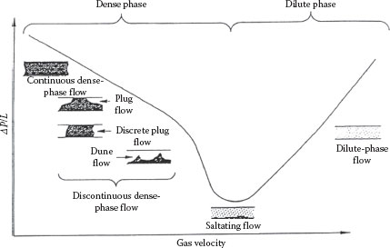
FIGURE 16.4 Pressure gradient–velocity relation for horizontal pneumatic flow.
Dilute Phase versus Dense Phase Pneumatic Transport
Conveying Mode |
Solids Loading (e.g., kgs/kgg) |
Conveying Velocity ft/s (m/s) |
ΔP psi (kPa) |
Solids Volume Fraction |
Dilute phase |
<15 |
>35 (10) |
<15 (100) |
<1% |
Dense phase |
>15 |
<35 (10) |
>15 (100) |
>30% |
Although a lot of information is available on dilute phase transport, which is useful for designing such systems, transport in the dense phase is much more difficult and more sensitive to detailed properties of the specific solids. Thus, because operating experimental data on the particular materials of interest are usually needed for dense phase transport, we will limit our treatment here to the dilute phase.
There are a variety of correlations for the saltation velocity, one of the most popular being that of Rizk (1973):
(16.27) |
where
and
(16.28) |
where
μs is the “solids loading” (mass of solids/mass of gas)
Vgs is the saltation gas velocity
d is the particle diameter (mm)
D is the pipe diameter
It should be pointed out that correlations such as this are based, of necessity, on a finite range of conditions and have a relatively broad range of uncertainty, for example, ±50%–60% is not unusual (see, e.g., the recent work of Wilms and Dhodapkar, 2014).
The two major effects that contribute to the pressure drop in horizontal flow are acceleration of the particles and friction loss. Initially, the inertia of the particles must be overcome as they are accelerated up to speed, and then the friction loss in the mixture must be overcome. If VS is the solid particle velocity and ṁS = ρSVSA(1–εm) is the solids mass flow rate, the acceleration component of the pressure drop is
(16.29) |
The slip ratio VG/VS = S can be estimated, for example, from the IGT correlation (e.g., Klinzing et al., 2010):
(16.30) |
in which
d and D are the particle and pipe diameters, respectively, in meters
ρS and ρG are in kg/m3
For vertical transport, the major differences are that no “bed” on the pipe wall is possible but, instead, the pressure gradient must overcome the weight of the solids as well as the fluid and the fluid/particle drag, so that the solids holdup and hence the fluid velocity must be significantly higher under transport conditions. The steady flow pressure drop in the pipe can be deduced from a momentum balance on a differential slice of the fluid–particle mixture in a constant diameter pipe, as was done in Chapter 5 for single-phase flow (see Figure E5.4). For steady uniform flow through area Ax:
(16.31) |
where
τwS and τwG are the effective wall stresses resulting from energy dissipation due to the particle–particle and particle–wall and gas–wall interactions
Wp is the wetted perimeter
Dividing by Ax, integrating, and solving for the pressure drop, −ΔP = P1 − P2, gives
(16.32) |
where Dh = 4Ax/Wp is the hydraulic diameter. The void fraction εm is the volume fraction of the gas in the pipe, i.e.,
(16.33) |
The wall stresses are related to the corresponding friction factors by
(16.34) |
Here ΔPfG is the pressure drop due to “gas only” flow (i.e., the gas flowing alone in the full pipe cross section). Note that if the pressure drop is less than about 30% of P1, the incompressible flow equations can be used to determine ΔPfG using the average gas density. Otherwise, the compressibility must be considered and the methods outlined in Chapter 9 must be used to determine ΔPfG. The pressure drop is related to the pressure ratio P1/P2 by
(16.35) |
The solids contribution to the pressure drop ΔPfS includes contributions from both the particle–wall and the particle–particle interactions. The latter is reflected in the dependence of the friction factor fS on the particle diameter, along with the drag coefficient, density, and the relative (slip) velocity (Hinkle, 1953):
(16.36) |
A variety of other expressions for fS have been proposed by various authors (see, e.g., Klinzing et al., 2010) and that of Yang (1983) for horizontal flow
(16.37) |
and for vertical flow
(16.38) |
where
(16.39) |
Vt is the particle terminal velocity.
The principles governing vertical pneumatic transport are the same as those given earlier, and the method for determining the pressure drop is identical (with an appropriate expression for fS). However, there is one major difference in vertical transport, which occurs as the gas velocity is decreased. As the velocity falls, the frictional pressure drop decreases but the slip increases since the drag force exerted by the gas entraining the particles also decreases. The result is an increase in the solids holdup, with a corresponding increase in the static head opposing the flow, which in turn causes an increase in the pressure drop. A point will be reached at which the gas can no longer entrain all of the solids and a slugging fluidized bed results with large pressure fluctuations. This condition is known as choking (not to be confused with choking that occurs when the gas velocity reaches the speed of sound) and represents the lowest gas velocity at which vertical pneumatic transport can be attained at a specified solids mass flow rate. The choking velocity, Vc, and the corresponding void fraction, εc, are related by the following two equations (Yang, 1983):
(16.40) |
and
(16.41) |
where ρo is the gas phase density at upstream conditions. These two equations must be solved simultaneously for Vc and εc.
IV. GAS–LIQUID TWO-PHASE PIPE FLOW
The two-phase flow of gases and liquids has been the subject of literally thousands of publications in the literature, and it is clear that we can only provide a brief introduction to the subject here. Although the single-phase flow of liquids and gases is relatively straightforward, the two-phase combined flow can be significantly more complex. Two-phase gas–liquid flows are also more complex than fluid–solid flows because of the wider variety of possible flow regimes and the possibility that the liquid may be volatile and/or the gas a condensable vapor, with the result that the mass ratio of the two phases may change throughout the system.
The configuration or distribution of the two phases in a pipe depends upon the phase ratio and the relative velocities of the two phases. These regimes can be described qualitatively as illustrated in Figure 16.5a for horizontal flow and Figure 16.5b for vertical flow. The patterns for horizontal flow are seen to be more complex than for vertical flow because of the asymmetric effect of gravity. The boundaries or transitions between these regimes have been mapped by various investigators based on observations in terms of various flow and property parameters. A number of these maps have been compared by Rouhani and Sohal (1983). Typical flow regime maps for horizontal and vertical flow are shown in Figure 16.6a and b. In Figures 16.5 and 16.6, GG = ṁG/A is the mass flux of the gas, GL = ṁL/A is the mass flux of the liquid, and λ and Φ are fluid property correction factors:
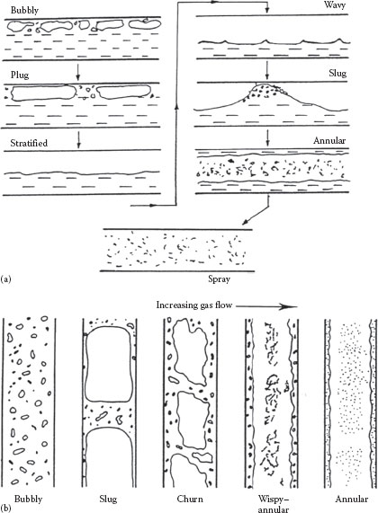
FIGURE 16.5 Flow regimes in (a) horizontal and (b) vertical gas–liquid flow.
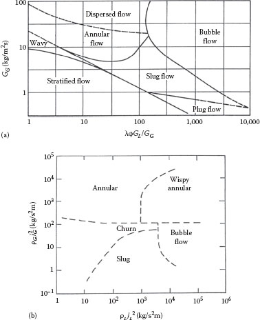
FIGURE 16.6 Flow regimes map for (a) horizontal and (b) vertical gas–liquid flow. (a: From Baker, O., Oil Gas J., 53, 185, 1954; b: From Hewitt, G.F. and Roberts, D.N., Studies of two-phase flow patterns by x-ray and flash photography, Report AERE-M 2159, HMSO, London, U.K., 1969.)
(16.42) |
(16.43) |
where
σ is surface tension
W and A subscripts refer to water and air, respectively, at 20°C
A quantitative model for predicting the flow regime map for horizontal flow in terms of five dimensionless variables has been developed by Taitel and Dukler (1976) and was further extended to any pipe inclination by Barnea (1987). The approach proposed in this work, referred to as “mechanistic models,” combines fluid flow equations describing different flow patterns, with closing relations, and has been further improved upon by many researchers (see, e.g., Zhang (2003) for additional details).
The momentum equation written for a differential length of pipe containing the two-phase mixture is similar to Equation 16.31, except that the rate of change of momentum changes along the tube due to the change in velocity as the gas or vapor expands as the pressure drops. For steady uniform flow through area Ax:
(16.44) |
where
τwL and τwG are the shear stresses exerted by the liquid and the gas on the wall
Wp is the wetted perimeter
Dividing by Ax dx and solving for the pressure gradient, −dP/dX gives
(16.45) |
where Dh = 4Ax/Wp is the hydraulic diameter. The total pressure gradient is seen to be composed of three terms resulting from the static head change (gravity), energy dissipation (friction loss), and acceleration (the change in kinetic energy), that is,
(16.46) |
which is equivalent to Equation 9.14 for pure gas flow.
B. HOMOGENEOUS GAS–LIQUID MODELS
In principle, the energy dissipation (friction loss) associated with the gas–liquid, gas–wall, and liquid–wall interactions can be evaluated separately and summed to get the total energy dissipation for the system. However, even for distributed (nonhomogeneous) flows, it is common practice to evaluate the friction loss as a single term which, however, depends in a complex manner upon the nature of the flow pattern and fluid properties in both phases. This is referred to as the “homogeneous” model:
(16.47) |
The homogeneous model also assumes both phases to be moving at the same velocity, that is, no slip. Since the total mass flux is constant, the acceleration (or kinetic energy change) term can be written:
(16.48) |
where νm = 1/ρm is the average specific volume of the homogeneous two-phase mixture
(16.49) |
and x is the quality (i.e., the mass fraction of gas). For “frozen” flows in which there is no phase change (e.g., air and cold water), the acceleration term is often negligible in steady pipe flow (although it can be appreciable in entrance flows and in non-uniform cross-section channels). However, if a phase change occurs (e.g., flashing of hot water or other volatile liquids), this term can be very significant. Evaluating the derivative of vm from the previous equation gives
(16.50) |
where vGL = vG – vL. The first term on the right describes the effect of the gas expansion on the acceleration for constant mass fraction and the last term represents the additional acceleration resulting from a phase change from liquid to gas (e.g., a flashing liquid).
Substituting the expressions for the acceleration and friction loss pressure gradients into the total pressure gradient equation and rearranging gives
(16.51) |
Finding the pressure drop corresponding to a total mass flux Gm from this equation requires a stepwise procedure using physical property data from which the density of both the gas phase and the mixture can be determined as a function of pressure. For example, if the upstream pressure P1 and the mass flux Gm are known, the equation is used to evaluate the pressure gradient at point 1 and hence the change in pressure ΔP over a finite length ΔL, and then the pressure P1+i = P1 – ΔP. The densities are then determined at pressure P1+i, and the process is repeated at successive increments until the end of the pipe is reached. If the flow is choked, the pressure gradient will tend toward infinity at the choke point.
There are a number of special cases that permit simplification of Equation 16.51. For example, if the pressure is high and the pressure gradient moderate, the term in the denominator that represents the acceleration due to gas expansion can be neglected. Likewise for “frozen” flow for which there is no phase change (e.g., air and cold water), the quality (x) is constant and the second term in the numerator is zero. For flashing flows, the change in quality with length (dx/dX) must be determined from a total energy balance from the pipe inlet (or stagnation) conditions, along with the appropriate vapor–liquid equilibrium data for the flashing liquid. If the Clausius–Clapeyron equation is used, this becomes
(16.52) |
where
λGL is the heat of vaporization
vGL is the change in specific volume due to vaporization
For an ideal gas,
(16.53) |
It should be noted that the derivative is negative, so that if conditions are such that if the denominator of Equation 16.51 is zero, an infinite pressure gradient would result. This condition corresponds to the speed of sound, that is, choked flow. For a nonflashing liquid and an ideal gas mixture, the corresponding maximum (choked) mass flux, , follows directly from the definition of the speed of sound
(16.54) |
The ratio of the sonic velocity in a homogeneous two-phase mixture to that in a gas alone is . This ratio can be much smaller than unity, so that choking can occur in a two-phase mixture at a higher downstream pressure than that for a singlephase gas flow (i.e., at a lower pressure drop and a corresponding lower mass flux).
Evaluation of each term in Equation 16.51 is straightforward, except for the friction factor. One approach is to treat the two-phase mixture as a “pseudo-single-phase” fluid with appropriate properties. The friction factor is found assuming the usual Newtonian methods (i.e., Moody diagram, Churchill equation) using a suitable Reynolds number, for example,
(16.55) |
where μm is an appropriate viscosity for the two-phase mixture. A wide variety of methods have been proposed for estimating this viscosity, but the one that seems most logical is the local volume-weighted average (Dukler et al., 1964b):
(16.56) |
The corresponding density ρm is the “no-slip” or equilibrium density of the mixture:
(16.57) |
Note that the frictional pressure gradient is inversely proportional to the fluid density for a given mass flux:
(16.58) |
The corresponding pressure gradient for purely liquid flow is
(16.59) |
Taking the reference liquid mass flux to be the same as that for the two-phase flow (GL = Gm) and the friction factors to be the same (fL = fm), then
(16.60) |
A similar relation could be written by taking the single-phase gas flow as the reference instead of the liquid, that is, GG = Gm. This is the basis for the two-phase multiplier method:
(16.61) |
where
R represents a reference single-phase flow
is the two-phase multiplier
There are four possible reference flows:
1. R = L: The total mass flow is liquid (Gm = GL).
2. R = G: The total mass flow is gas (Gm = GG).
3. R = LLm: The total mass flow is that of the “liquid only” in the mixture (GLm = (1 – x)Gm).
4. R = GGm: The total mass flow is that of the “gas only” in the mixture (GGm = xGm).
The two-phase multiplier method is utilized primarily for separated flows, which will be discussed later.
1. Omega Method for Homogeneous Equilibrium Flow
For homogeneous equilibrium (no slip) flow in a uniform pipe, the governing (Bernoulli) equation can be written (equivalent to Equation 16.45) as
(16.62) |
where vm = 1/ρm. By integrating over the pipe length, L, and assuming the friction factor to be constant, this can be rearranged as follows:
(16.63) |
where X is the distance along the pipe. Leung (1996) utilized a linearized two-phase equation of state to evaluate vm = fn(P):
(16.64) |
where ρo is the two-phase density at the upstream (stagnation) pressure Po. The parameter ω represents the compressibility of the fluid and can be determined from property data for ρ = fn(P) at two pressure values or estimated from the physical properties at the upstream (stagnation) state. This equation is based on the fact that isentropic lines for most single-component fluids in the vapor–liquid two-phase region are almost linear in the coordinates (1/P, ν). The parameter ω is the inverse value of the isentropic exponent in the two-phase region (ω = 1/kPρ, see Chapter 9) and can be calculated using the following equations:
For any flashing system
(16.65) |
where and are the dimensionless thermal expansion coefficient and isothermal bulk modulus, respectively. For an ideal gas, , and
(16.66) |
For nonflashing (frozen) flows of an ideal gas and liquid:
(16.67) |
Using Equation 16.64, Equation 16.63 can be written as
(16.68) |
where η = P/Po, G* = Gm/(Poρo)1/2 and
(16.69) |
is the “flow inclination number.” From the definition of the speed of sound, it follows that the exit pressure ratio at which choking occurs is given by
(16.70) |
For horizontal flow, Equation 16.68 can be evaluated analytically to give
(16.71) |
As ω → 1 (i.e., setting ω = 1.001 in Equation 16.71), this reduces to the solution for ideal isothermal gas flow (Equation 9.17), and for ω = 0, it reduces to the incompressible flow solution. For inclined pipes, Leung (1996) has given the solution of Equation 16.68 in graphical form for various values of NFi.
A so-called universal equation for designing pipelines for two-phase flow has been presented by Kim et al. (2015). This method is basically an extension of the Leung omega method, which utilizes average values of the density and specific volume over the pressure range of interest in terms of two empirical parameters determined by a fit of ρ versus P data. This method is not applicable to subcooled flashing flows.
It is also possible to use Equations 9.97 and 9.98 for two-phase homogeneous equilibrium flow in the region where isentropic exponents and coefficients in these equations change slowly (which is usually the case for values that are not too small, that is, where ω = 1/kPρ ≤ 2).
For single-component flashing flow, kPρ = ω−1 so that, in this case, ω can be calculated by Equation 16.65 and kTP = PoνGLo/λGLo. Equation 9.96 also can be used for two-phase flow with a simple approximation ω = 1/kPρ ≤ 2.
2. Generalized (Homogeneous Direct Integration) Method for All Homogeneous Flow Conditions
The omega method is limited to systems for which the linearized two-phase equation of state (Equation 16.64) is a good approximation to the two-phase density (i.e., single-component systems and multicomponent mixtures of similar compounds). Fluid property data for ρ versus P for at least two values of P are required to evaluate the parameter ω.
For any system (including single- or two-phase and frozen or flashing flows), the governing equations for homogeneous flow can be evaluated numerically using either experimental or theoretical (EOS) thermodynamic properties for the P–ρ relation.
For example, the basic Bernoulli equation for pipe flow can be integrated and rearranged to give
(16.72) |
where the right-hand side of Equation 16.72 incorporates the finite difference version of the integral. This method is referred to as the homogeneous direct integration (HDI) method and is similar to that for sizing relief valves for homogeneous flow. The term includes the pipe loss coefficient (i.e., Kpipe = 4fL/D) as well as any fittings in the line.
A thermodynamic property database is used to evaluate the mixture density as a function of pressure at suitable pressure intervals along an adiabatic path from P1 to P2. An adiabatic path is more appropriate for pipe flow, as opposed to an isentropic path as used for relief valve nozzles. However, as the pipe length increases, adiabatic flow approaches isothermal flow (see Figure 9.3). Alternately, an isentropic path can be used for the numerical approximation, as the friction loss term, , represents the irreversible nonisentropic contribution to the integral. By starting at P2 = P1 values of G are calculated from Equation 16.72 as P2 is reduced until the exit pressure is reached. If the value of G reaches a maximum before the exit pressure is reached, then the flow is choked at that value of G and the corresponding value of P2 is the choke pressure, Pc. This method can be applied directly to single- or multiphase fluids and frozen or flashing flows as long as suitable property data are available. Multicomponent fluids require an adiabatic flash routine to determine the required P(ρ) function. A good inexpensive thermodynamic database for many single-component and some multicomponent fluids that can be used for this purpose is the NIST Database (NIST, 2015).
Homogeneous flow models apply when the velocity of the two-phase mixture is large enough that turbulence will mix the two phases sufficiently that the mixture can be described as a “pseudo-single-phase” fluid, with appropriate “average” physical properties of the mixture.
At lower flow rates, the fluids will flow as separate phases, each occupying a specific portion of the flow field. Separated flow models consider each phase to occupy a defined fraction of the flow cross section and account for possible differences in the phase velocities (i.e., slip). There are a variety of such models in the literature, and many of these have been compared against data for various horizontal flow regimes by Chisholm (1983), Dukler et al. (1964a) and later by Ferguson and Spedding (1995).
The “classic” Lockhart–Martinelli (1949) method is based upon the two-phase multiplier defined previously for either “liquid only” (Lm) or “gas only” (Gm) reference flows, that is,
(16.73) |
or
(16.74) |
where
(16.75) |
and
(16.76) |
Here, Φ is the two-phase multiplier, which is correlated as a function of the Lockhart–Martinelli correlating parameter χ2, defined as
(16.77) |
The correlation is shown in Figure 16.7. There are four curves for each multiplier, depending upon the flow regime in each phase, that is, both turbulent (tt), both laminar (vv), liquid turbulent and gas laminar (tv), or liquid laminar and gas turbulent (vt). The curves can also be represented by the following equations:
(16.78) |
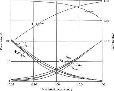
FIGURE 16.7 Lockhart–Martinelli two-phase correlating parameters.
Values of Constant C in Two-Phase Multiplier Equations
Flow State |
Liquid |
Gas |
C |
tt |
Turbulent |
Turbulent |
20 |
vt |
Laminar |
Turbulent |
12 |
tv |
Turbulent |
Laminar |
10 |
vv |
Laminar |
Laminar |
5 |
and
(16.79) |
where the values of C for the various flow combinations are shown in Table 16.2.
Here fLm is the pipe friction factor based on the “liquid only” Reynolds number NReLm = (1 – x) GmD/μL and fGm is the friction factor based on the “gas only” Reynolds number NReGm = xGmD/μG. The curves cross at χ = 1, and it is best to use the “G” reference curves if χ < 1 and the “L” curves for χ > 1.
Using similar analysis, Duckler et al. (1964a,b) deduced that
(16.80) |
or
(16.81) |
which is equivalent to the following Martinelli parameters:
(16.82) |
where
(16.83) |
and
Here φ and ρ are the equilibrium (“no slip”) properties. Another major difference is that Duckler deduced that the friction factors fL and fG should both be evaluated at the following mixture Reynolds number:
(16.84) |
A major complication, especially for separated flows, arises from the effect of slip in gas/liquid flows. Slip occurs because the less dense and less viscous phase exhibits a lower resistance to flow, as well as expansion and acceleration of the gas phase as the pressure drops along the pipe length. The net result is an increase in the local holdup of the more dense phase within the pipe (φm) (or the corresponding two-phase density, ρm), as given by Equation 16.11. A large number of expressions and correlations for the holdup or (equivalent) slip ratio have appeared in the literature, and that deduced by Lockhart and Martinelli is shown in Figure 16.7. Many of these slip models can be summarized in terms of a general correlation of the form
(16.85) |
where the values of the parameters are shown in Table 16.3.
Although many additional slip models have been proposed in the literature, it is not clear which of these should be used under any given set of circumstances. In some cases, a constant slip ratio (S) may give satisfactory results. For example, a comparison of calculated and experimental mass flux data for high velocity air–water flows through nozzles (Jamerson and Fisher, 1999) found that S = 1.1–1.8 accurately represents the data over a range of x = 0.02–0.2, with the value of S increasing as the quality (x) increases.
A general correlation for slip has been given by Butterworth and Hewitt (1977):
(16.86) |
where
(16.87) |
(16.88) |
(16.89) |
(16.90) |
Parameters for Slip Model Equation (16.85)
Model |
ao |
a1 |
a2 |
a3 |
Homogeneous |
1 |
1 |
1 |
0 |
S = (ρL/ρG)½ (Fauske, 1962) |
1 |
1 |
1/2 |
0 |
S = (ρL/ρG)⅓ (Moody, 1965) |
1 |
1 |
2/3 |
0 |
Thom (1964) |
1 |
1 |
0.89 |
0.18 |
Baroczy (1966) |
1 |
0.74 |
0.75 |
0.13 |
Lockhart–Martinelli (t-t) (1949) |
1 |
0.75 |
0.417 |
0.083 |
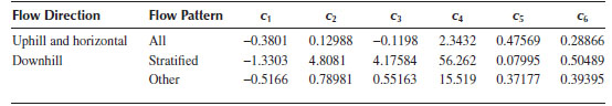
An empirical correlation of holdup was developed by Mukherjee and Brill (1983) based on more than 1500 measurements of air with oil and kerosene in horizontal, inclined, and vertical flow (inclination of ±90°). Their results for the holdup were correlated by an empirical equation of the form
(16.91) |
where
and σ is the liquid surface tension. The constants in Equation 16.91 are given in Table 16.4 for the various flow inclinations.
A correlation for holdup by Hughmark (1962) was found to represent data quite well for both horizontal and vertical gas–liquid flow over a wide range of conditions. This was found by Dukler et al. (1964a) to be superior to a number of other relations that were checked against a variety of data sets. The Hughmark (1962) correlation is equivalent to the following expression for slip:
(16.92) |
The parameter K was found to correlate well with the dimensionless parameter Z:
(16.93) |
where ε is the “no-slip” volume fraction of gas. The volume average viscosity of the two phases is used in the Reynolds number, and NFr = V2/gD, where V is the average velocity of the two-phase mixture. Hughmark (1962) presented the correlation between K and Z in graphical form, which can be represented quite well by the expression:
(16.94) |
Coefficients for Equation 16.91
Slip is related to the holdup by Equation (16.13). The presence of slip also means that the acceleration term in the governing equation (Equation 16.45) cannot be evaluated in the same manner as for homogeneous flow conditions. When the acceleration term is expanded to account for the difference in phase velocities, the momentum equation when solved for the total pressure gradient becomes
(16.95) |
where
(16.96) |
The pressure drop over a given length of pipe must be determined by a stepwise procedure, as described for homogeneous flow. The major additional complication in this case is the evaluation of the holdup (φm, or the equivalent slip ratio S) using one of the aforementioned correlations.
In some special cases, simplifications are possible, which makes the process easier, such as
1. If the denominator of Equation 16.95 is close to unity
2. If fm, ρL, and ρG are nearly constant over the length of pipe
Example 16.2
Estimate the pressure gradient (in psi/ft) for a two-phase mixture of air and water entering a horizontal 6 in. sch 40 pipe at a total mass flow rate of 6500 lbm/min at 150 psia, 60°F, with a quality (x) of 0.1 (mass fraction of air). Compare your answer using the (a) Omega, (b) Lockhart–Martinelli, (c) Dukler, and (d) HDI methods.
Solution
At the entering temperature and pressure, the density of air is 0.7799 lbm/ft3, its viscosity is 0.02 cP, the density of water is 62.4 lbm/ft3, and its viscosity is 1 cP. The no-slip volume fraction corresponding to the given quality is (by Equation 16.11) 0.899, and the corresponding density of the mixture (by Equation 16.12) is 7.01 lbm/ft3. The viscosity of the mixture by Equation 16.56 is 0.119 cP. The slip ratio can be estimated from Equation 16.85 using the Lockhart–Martinelli constants from Table 16.3 to be S = 10.28. Using this value in Equation 16.13 gives the in situ holdup φm = 0.6027. From the given mass flow rate and diameter, the total mass flux Gm = 540 lbm/ft2 s.
(a) Omega method: Since this is a “frozen” flow (no phase changes), the value of ω is given by Equation 16.67, with k = 1.4 for air, which gives ω = 0.642. From the given data, NRem = D Gm/μm = 3.41 × 10⁶, which, assuming a pipe roughness of 0.005 in., gives f = 0.00412 and a value of 4fL/D = 0.0326. The pressure gradient is determined from Equation 16.70, with G* = Gm/(Poρo)½ = 0.245 and η1 = 1. The equation is solved by iteration for η2 = 0.999 or P2 = 149.9 psia. The pressure gradient is thus (P1 − P2)/L = 0.0969 psi/ft. This pressure gradient will apply until the pressure drops to the choke pressure, which from Equation 16.70 is 7.19 psia.
(b) Lockhart–Martinelli method: Using the “liquid only” basis, the corresponding Reynolds number is NReLm = (1 – x)DGm/μL = 3.66 × 10⁵, which gives a value of fLm = 0.00419. Likewise, using the “gas only” basis gives NReGm = xDGm/μG = 2.27 × 10⁶, which gives fGm = 0.00383. These values give the corresponding pressure gradients from Equations 16.76 and 16.77 as 0.0135 and 0.012 psi/ft, respectively. The square root of the ratio of these values gives the Lockhart–Martinelli parameter χ = 1.0527, which, from Equation 16.73, gives . The pressure gradient is then calculated from Equation 16.76 to be 0.283 psi/ft.
(c) Duckler method: This method requires determining values for β and α from Equation 16.83. The in-situ holdup determined earlier, φm = 0.6027, is used in the equation for β to give a value of 0.377, and the “no-slip” holdup value of φ = 0.101 is used in the equation for α to give a value of 2.416. These values are used in Equation 16.80, with a value of f = 0.00378, to determine the pressure gradient of 0.122 psi/ft.
(d) HDI method: For this problem, Equation 16.51 can be used. For horizontal flow (dz = 0) and constant quality (x), this equation reduces to
(16.97) |
Finding the pressure drop corresponding to a total mass flux Gm from this equation requires a stepwise procedure using physical property data from which the density of both the gas phase and the mixture can be determined as a function of pressure. For example, if the upstream pressure P1 and the mass flux Gm are known, the equation is used to evaluate the pressure gradient at point 1 and hence the change over a finite pipe length ΔL for the pressure increment ΔP and then at the pressure P1+i + = P1 – ΔP. The densities are then determined at pressure P1+i, and the process is repeated at successive increments until the end of the pipe is reached. Assuming isothermal flow, the density (and specific gravity) of the two-phase mixture will vary down the pipe as the pressure drops and the air expands. The properties of air can be accessed by the NIST Database, over the pressure range of 150–14.7 psia at 2 psi increments, and used to calculate the specific volume of the mixture from
Alternately, the air can be assumed to be an ideal gas and its density calculated accordingly (in this example, the ideal gas law is an excellent approximation). A pressure increment of 2 psi is selected, and the density (and/or specific volume) of the mixture is tabulated in the spreadsheet as a function of pressure from 150 to 14.7 psia. This requires a determination of the pipe friction factor that depends on the Reynolds number, which, in turn, depends on the mixture viscosity, which is unknown, that is, NRe = DG/μ.
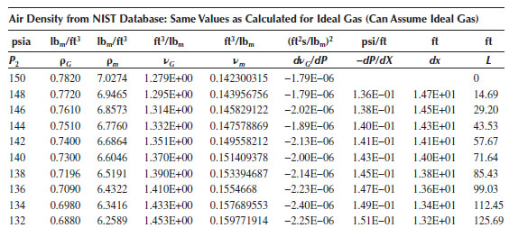
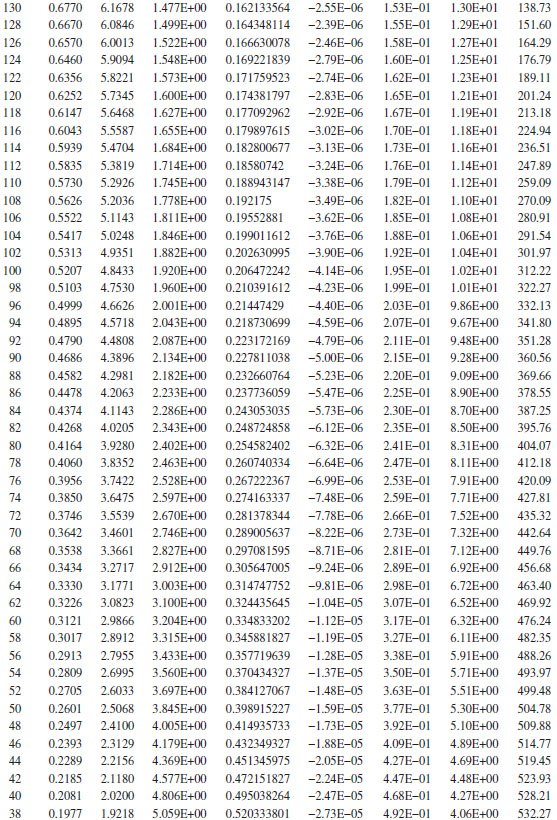
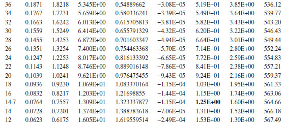
If a reasonable “guesstimate” is made for the viscosity, for example, 20 cP, and the pipe roughness is assumed to be 0.0018 in., the resulting value of the friction factor is found to be about 0.0038. The pressure gradient is found as a function of P from Equation (16.51), which can then be used to determine ΔX (and L) versus P. As L increases, the pressure gradient increases, and as the flow approaches choked, the pressure gradient approaches infinity. The spreadsheet output for this problem is shown above, which indicates that at the end of the pipe (L = 565 ft, P2 = 14.7 psia), the pressure gradient is 1.25 psi/ft. Note the pressure gradient at the pipe entrance is 0.136 psi/ft, and at the end of the pipe, it is 1.25 psi/ft. An increase of almost a factor of 10 indicates that the flow is almost at the choke pressure at the pipe exit.
The flow regime can be determined from Figure 16.6a using an ordinate of 1 and an abscissa of 2635 kg/m2s, to be well in the dispersed flow regime, so each of these methods should be applicable.
The following points should be retained from this chapter:
• Understand the definitions of the various measures of mass flux, volume flux, phase velocity and slip concentrations of the heavier and lighter phases in two-phase solid–liquid and gas/vapor–liquid flows.
• Know how to determine the pressure drop in a pipe for homogeneous and heterogeneous (separated) (gas/vapor)/liquid and solid–liquid flows.
• Understand the difference in the mechanisms for dense phase and dilute phase pneumatic transport, as well as horizontal versus vertical transport.
• Recognize the difference in flow regimes for horizontal and vertical gas–liquid pipe flows.
1. An aqueous slurry contains 45% (vol.) solids, with SG = 4 and psd given below. The slurry is a Bingham plastic, with properties given below. Calculate the pressure gradient (psi/ft) for the slurry at 8 ft/s in a 10 in. ID pipe.
The procedure is the same as that outlined in Example 15.1, using the Molerus state diagram for the heterogeneous component and the Bingham plastic pipe flow equations for the homogeneous component. The terminal velocity of the largest particles is found using the correlation for Bingham plastic in Chapter 11. A “no solution” is obtained from this correlation for conditions corresponding to particles which are too small to fall in the Bingham fluid, which sets the division between the heterogeneous and homogeneous regions, and the respective solids size and concentration. The concentration of solids in the homogeneous fraction is used to calculate the density of this phase.
US Screen Mesh |
Mesh Opening (μm) |
Fraction Passing |
400 |
37 |
0.05 |
325 |
44 |
0.05 |
200 |
74 |
0.05 |
140 |
105 |
0.05 |
100 |
149 |
0.05 |
60 |
250 |
0.1 |
35 |
500 |
0.1 |
18 |
1000 |
0.15 |
10 |
2000 |
0.2 |
5 |
4000 |
0.2 |
Slurry pipe flow |
|
Given: |
Total solids fraction: Cv = 0.45 Cvcont = 0.369 Bingham properties: τo = 5 dyn/cm2 μ∞ = °.3 P ρs = 3 g/cm3, ρL = 1 g/cm3 ρm = 1.738 g/cm3 S = 1.726122 ρs/ρm Pipe D = 18 in. V = 8 ft/s ρm = ρsCv + ρL(1 – Cv) |
2. An aqueous slurry contains 45% (vol.) solids, with SG = 4 and psd the same as in Problem 1. The slurry is a power law fluid, with properties given. Calculate the pressure gradient (psi/ft) for the slurry at 8 ft/s in a 10 in. ID pipe.
The procedure is the same as that outlined in Example 16.1, using the Molerus state diagram for the heterogeneous component and the power law pipe flow equations for the homogeneous component. The terminal velocity of the largest particles is found using the correlation for power law fluid in Chapter 11.
Slurry pipe flow |
|
Given: |
Total solids fraction: Cv = 0.45 Cvcont = 0.4095 Power law properties: m = 60 poise n = 0.18 ρs = 4 g/cm3 ρL = 1 g/cm3 ρm = 2.2285 g/cm3 S = 1.795 ρs/ρm Pipe D = 18 in. V = 8 ft/s ρm = ρsCv + ρL(1 – Cv |
3. An aqueous slurry is composed of 45% solids (by volume). The solids have an SG of 4 and a particle size distribution shown here:
US Screen Mesh |
Mesh Opening (μm) |
Fraction Passing |
400 |
37 |
0.02 |
325 |
44 |
0.06 |
200 |
74 |
0.08 |
140 |
105 |
0.10 |
100 |
149 |
0.15 |
60 |
250 |
0.18 |
35 |
500 |
0.20 |
18 |
1000 |
0.12 |
10 |
2000 |
0.08 |
5 |
4000 |
0.01 |
The slurry behaves as a non-Newtonian fluid, which can be described as a Bingham plastic with a yield stress of 40 dyn/cm2 and a limiting viscosity of 100 cP. Calculate the pressure gradient (in psi/ft) for this slurry flowing at a velocity of 8 ft/s in a 10 in. ID pipe.
4. Spherical polymer pellets with a diameter of 1/8 in. and an SG of 0.96 are to be transported pneumatically using air at 80°F. The pipeline is horizontal, 6 in. ID and 100 ft long, and discharges at an atm pressure. It is desired to transport 15% by volume of solids at a velocity that is 1 ft/s above the minimum deposit velocity.
(a) What is the pressure of the air that is required at the entrance to the pipe to overcome the friction loss in the pipe? (Note: There is an additional pressure gradient required to accelerate the particles after contacting with the air, but your answer should address only the friction loss).
(b) If a section of this pipe is vertical, what would the choking velocity be in this line and the pressure gradient (in psi/ft) at a velocity of 1 ft/s above this velocity?
5. Saturated ethylene enters a 4 in. sch 40 pipe at 400 psia. The ethylene flashes as the pressure drops through the pipe, and the quality at any pressure can be estimated by assuming constant enthalpy along the pipe. If the pipe is 80 ft long and discharges at a pressure of 100 psia, what is the mass flow rate through the pipe? Use 50 psi pressure increments in the stepwise calculation procedure.
6. A two-phase mixture of natural gas (methane) and a 40°API liquid are being pumped through a 6 in. sch 40 pipeline at 80°F. The mixture enters the pipe at 500 psia at a total rate of 6000 lbm/min and 6% quality. What is the total pressure gradient in the pipe at this point (in psi/ft)?
7. Repeat Example 16.2 using the HDI method, and compare the results with the other methods used in this example.
Ax |
x-component of area, [L2] |
a |
Slip correlating parameter, Equation 16.86, [—] |
b |
Slip correlating parameter, Equation 16.88, [—] |
c |
Speed of sound, [L/t] |
Cd |
Particle drag coefficient, [—] |
Cp |
Specific heat, [F L/(M T) = L2/(t2 T)] |
D |
Pipe diameter, [L] |
Dh |
Hydraulic diameter, [L] |
d |
Particle diameter, [L] |
F |
Force, [F = M L/t2] |
f |
Fanning friction factor, [—] |
G |
Mass flux, [M/(L2 t)] |
G* |
Dimensionless mass flux, [—] |
g |
Acceleration due to gravity, [L/t2] |
J |
Volume flux (superficial velocity), [L/t] |
k |
Isentropic exponent (specific heat ratio for ideal gas), [—] |
K |
εm/ε, parameter in Hughmark correlation, Equation 16.92, [—] |
L |
Pipe length, [L] |
ṁ |
Mass flow rate, [M/t] |
NFi |
Flow inclination number, Equation 16.69 [—] |
NFr |
Froude number, [—] |
NFrp |
Particle Froude number, Equation 16.22, [—] |
NFrs |
Solids Froude number, Equation 16.28, [—] |
NFrt |
Pipe Froude number, Equation 16.23, [—] |
NRe |
Reynolds number, [—] |
NRet |
Particle terminal velocity Reynolds number, Equation 16.39, [—] |
NRep |
Particle relative velocity Reynolds number, Equation 16.39, [—] |
NRe,TP |
Two-phase Reynolds number, [—] |
NWe |
Weber number, Equation 16.90, [—] |
P |
Pressure, [F/L2 = m/(L t2)] |
Q |
Volumetric flow rate, [L3/t] |
S |
Velocity slip ratio, [—] |
s |
ρS/ρL, [—] |
V |
Velocity, [L/t] |
Vc |
Choke velocity for vertical pneumatic transport, [L/t] |
V* |
Friction velocity, Equation 16.18, [L/t] |
Vgs |
Saltation gas velocity, [L/t] |
Vm |
Velocity of mixture, [L/t] |
Vmd |
Minimum deposit velocity, [L/t] |
Vr |
Relative (slip) velocity, [L/t] |
Dimensionless slip velocity, Vr/Vm, [—] |
|
Dimensionless single-particle slip velocity, Equation 16.24 |
|
Vt |
Particle terminal velocity, [L/t] |
WP |
Wetted perimeter, [L] |
X |
Dimensionless solids contribution to pressure drop, Equation 16.26, [—] |
X |
Horizontal coordinate direction, [L] |
Xo |
Dimensionless parameter defined by Equation 16.25, [—] |
x |
Mass fraction of less dense phase (quality, for gas–liquid flow), [—] |
Y |
Slip correlating parameter, Equation 16.87, [—] |
z |
Vertical direction measured upward, [L] |
Z |
Hughmark dimensionless parameter, defined by Equation 16.93 |
GREEK
α |
Volume fraction of gas phase, [—] |
Dimensionless thermal expansion coefficient, [—] |
|
δ |
Parameter defined in Equation 16.27, [—] |
χ2 |
Lockhart–Martinelli two-phase correlating parameter, Equation 16.77 [—] |
η |
Pressure ratio P/Po, [—] |
ΔPSi |
Contribution to total pressure drop by particle size fraction Si, [F/L2] |
Δz |
Increase in vertical position, [L] |
ε |
Volume fraction of the continuous phase, [—] |
εc |
Void fraction at choke point for vertical pneumatic transport, [—] |
εm |
Local value of ε at a specific point in pipe, [—] |
φm |
Local value of Ψ at a specific point in pipe, [—] |
Φ |
Property correction factor for gas/liquid flow regimes, Equation 16.43, [—] |
Two-phase multiplier with reference to single-phase R, Equation 16.61, [—] |
|
φ |
Volume fraction of the distributed phase, [—] |
Dimensionless isothermal bulk module, [—] |
|
λ |
Latent heat, [F L/M = L2/t2] |
λ |
Density correction factor, Equation 16.42, [—] |
λ |
Parameter for liquid/gas flow regimes, Equation 16.42 |
η |
Pressure ratio, [—] |
μ |
Viscosity, [M/(L t)] |
μs |
Solids loading (mass of solids/mass of gas) in pneumatic transport, [—] |
μs |
Ratio of mass of solids to mass of gas, [—] |
v |
Specific volume, [L3/M] |
ρ |
Density, [M/L3] |
σ |
Surface tension, [F/L = M/t2] |
τ |
Shear stress, [F/L2 = m/(L t2)] |
ω |
Two-phase equation of state parameter, Equation 16.64, [—] |
SUBSCRIPTS
1,2 |
Reference points |
C |
Choking condition |
f |
Friction loss |
G |
Gas |
L |
Liquid |
m |
Mixture |
Aude, T.C., N.T. Cowper, T.L. Thompson, and E. Wasp, Slurry piping systems: Trends, design methods, guidelines, Chem. Eng., 78, 74–90, June 28, 1971.
Baker, O., Simultaneous flow of oil and gas, Oil Gas J., 53, 185–195, 1954.
Barnea, D., A unified model for prediction flow-pattern transitions for the whole range of pipe inclinations, Int. J. Multiphase Flow, 13(1), 1–12, 1987.
Baroczy, C.J., A systematic correction for two-phase pressure drop, CEP Symp. Ser. 62(44), 232–249, 1966.
Brown, N.P. and N.I. Heywood, (Eds.), Slurry Handling: Design of Solid–Liquid Systems, Elsevier, London, U.K., 1991.
Butterworth, D. and G.F. Hewitt, (Eds.), Two-Phase Flow and Heat Transfer, Oxford University Press, Oxford, U.K., 1977.
Chisholm, D., Two-Phase Flow in Pipelines and Heat Exchangers, The Institution of Chemical Engineers, George Goodwin, London, U.K., 1983.
Center for Chemical Process Safety (CCPS), Guidelines for Pressure Relief and Effluent Handling Systems, AIChE, New York, 1998.
Darby, R., Hydrodynamics of slurries and suspensions, Chapter 2, in Encyclopedia of Fluid Mechanics, Vol. 5, N.P. Cheremisinoff, (Ed.), Gulf Publishing Co., Houston, TX, 1985.
Dukler, A.E., M. Wicks, III, and R.G. Cleveland, Frictional pressure drop in two-phase flow: A. A comparison of existing correlations for pressure loss and holdup, AIChE J., 10, 38–43, 1964a.
Dukler, A.E., M. Wicks, III, and R.G. Cleveland, Frictional pressure drop in two-phase flow: B. An approach through similarity analysis, AIChE J., 10, 44–51, 1964b.
Fan, L.-S. and C. Zhu, Principles of Gas-Solid Flows, Cambridge University Press, Cambridge, U.K., 1998.
Fauske, H.K., Contribution to the theory of two-phase, one-component critical flow, Argonne National Laboratory Report SNL-6673, October 1962.
Ferguson, M.E.G. and P.L. Spedding, Measurement and prediction of pressure drop in two-phase flow, J. Chem. Tech. Biotechnol., 62, 262–278, 1995.
Govier, G.W. and K. Aziz, The Flow of Complex Mixtures in Pipes, Van Nostrand Reinhold, 1983
Hanks, R.W., ASME Paper No. 80-PET-45, ASME Energy Sources Technology Conference, New Orleans, LA, February 3–7, 1980.
Hetsroni, G., (Ed.), Handbook of Multiphase Systems, McGraw Hill, New York, 1982.
Hewitt, G.F. and D.N. Roberts, Studies of two-phase flow patterns by x-ray and flash photography, Report AERE-M 2159, HMSO, London, U.K., 1969.
Hinkle, B.L., Acceleration of particles and pressure drops encountered in horizontal pneumatic conveying, PhD Thesis, Georgia Institute of Technology, Atlanta, GA, June 1953.
Hughmark, G.A., Holdup in gas-liquid flow, Chem. Eng. Prog., 58(4), 62–65, 1962.
Jamerson, S.C. and H.G. Fisher, Using constant slip ratios to model non-flashing (frozen) two-phase flow through nozzles, Process Safety Progress, 18(2), 89–98, 1999.
Kim, J.S., T. Oh, and H.J. Dunsheath, A universal equation for designing pipelines, Chem. Eng., 122, 66–71, September 10, 2015.
Klinzing, G.E., R.D. Marcus, F. Rizk, and L.S. Leung, Pneumatic Conveying of Solids, 3rd edn., Springer, Berlin, Germany, 2010.
Leung, J.C., Easily size relief devices and piping for two-phase flow, Chem. Eng. Prog., 92, 28–50, December 1996.
Levy, S., Two-Phase Flow in Complex Systems, Wiley, New York, 1999.
Lockhart, R.W. and R.C. Martinelli, Proposed correlation of data for isothermal two-phase, two-component flow in pipes, Chem. Eng. Prog., 45(1), 39–48, 1949.
Michaelides, E.E., J.D. Schwarzkopf and C. Crowe, Multiphase Flow Handbook, 2nd edn., CRC Press, Boca Raton, FL, 2016.
Molerus, O., Principles of Flow in Disperse Systems, Chapman & Hall, London, U.K., 1993.
Moody, F.J., Maximum flow rate of a single component two-phase mixture, Trans. ASME, J. Heat Trans., 87, 134–142, February, 1965.
Mukherjee, H. and J.P. Brill, Liquid holdup correlations for inclined two-phase flow, J. Petrol. Technol., 35, 1003–1008, May, 1983.
NIST (National Institute of Standards and Technology), REFPROP, version 9.5, Washington, DC, 2015.
Rizk, F., Dissertation, University of Karlsruhe, Karlsruhe, Germany, 1973.
Rouhani, S.Z. and M.S. Sohal, Two-phase flow patterns: A review of research results, Prog. Nucl. Energy, 11(3), 219–259, 1983.
Shook, C.A. and M.C. Roco, Slurry Flow—Principles and Practice, Butterworth-Heinemann, Boston, MA, 1991.
Taitel, Y. and A.E. Dukler, A model for predicting flow regime transitions in horizontal and near horizontal gas-liquid flow, AIChE J., 22(1), 47–55, 1976.
Thom, J.R.S, Prediction of pressure drop during forced circulation boiling of water, Intl. J. Heat Mass Transfer, 7, 709–724, 1964.
Wallis, G.B., One-Dimensional Two-Phase Flow, McGraw-Hill, New York, 1969.
Wasp, E.J., J.P. Kenny, and R.L. Gandhi, Solid-Liquid Flow in Slurry Pipeline Transportation, Trans-Tech Publications, Clausthal, Germany, 1977.
Wilms, H. and S. Dhodapkar, Pneumatic conveying: Optimal system design, operation and control, Chem. Eng., 121, 59–67, October, 2014.
Wilson, K.C., G.R. Addie, A. Sellgren, and R. Clift, Slurry Transport using Centrifugal Pumps, 3rd edn., Springer, New York, 2008.
Yang, W.C., Criteria for choking in vertical pneumatic conveying lines, Powder Technol., 35, 143–150, 1983.
Zhang, Y.-Q., Q. Wang, C. Sarica, and J.P. Brill, Unified model for gas-liquid pipe flow via slug dynamics—Part 1: Model development, Trans. ASME, 125, 266–273, 2003.
“It is better to know how to learn, than it is to know.”
—Dr. Seuss