1.7. Random Vector and Matrix Generation

For various simulation or power studies, it is often necessary to generate a set of random vectors or random matrices. It is therefore of interest to generate these quantities for the probability distributions which arise naturally in the multivariate normal theory. The following sections consider the most common multivariate probability distributions.

1.7.1. Random Vector Generation from N_p(μ, Σ)

To generate a random vector from N_p(μ, Σ) use the following steps:

The resulting vector y is an observation from a N_p(μ, Σ) population. To obtain a sample of size n, we repeat the above-mentioned steps n times within a loop.

1.7.2. Generation of Wishart Random Matrix

To generate a matrix A₁ ~ W_p(f, Σ), use the following steps:

The generation of Beta matrices can easily be done by first generating two independent Wishart matrices with appropriate degrees of freedom and then forming the appropriate products using these matrices as defined in Section 1.4.

EXAMPLE 2

Random Samples from Normal and Wishart Distributions In the following example we will illustrate the use of PROC IML for generating samples from the multivariate normal and Wishart distributions respectively. These programs are respectively given as Program 1.4 and Program 1.5. The corresponding outputs have been omitted to save space.

As an example, suppose we want to generate four vectors from N₃(μ, Σ) where

μ =(1 3 0)′

and

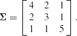
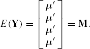
Then save these four vectors as the rows of 4 by 3 matrix Y. It is easy to see that

Also, let G be a matrix such that Σ = G′G. This matrix is obtained using the ROOT function which performs the Cholesky decomposition of a symmetric matrix.

/* Program 1.4 */

options ls = 64 ps=45 nodate nonumber;
    title1 'Output 1.4';

    /* Generate n random vector from a p dimensional population
    with mean mu and the variance covariance matrix sigma */

    proc iml ;
    seed = 549065467 ;
    n = 4 ;
    sigma = { 4 2 1,
              2 3 1,
              1 1 5 };

    mu = {1, 3, 0};
    p = nrow(sigma);
    m = repeat(mu`,n,1) ;
        g =root(sigma);
    z =normal(repeat(seed,n,p)) ;
    y = z*g + m ;
    print 'Multivariate Normal Sample';
    print y;

We first generate a 4 by 3 random matrix Z, with all its entries distributed as N(0,1). To do this, we use the normal random number generator (NORMAL) repeated for all the entries of Z, through the REPEAT function. Consequently, if we define Y = ZG + M, then the i^th row of Y, say y′_i, can be written in terms of the i^th row of Z, say z_i′, as

y′_i = z′_iG + μ′

or when written as a column vector

y_i = G′z_i + μ.

Consequently, y_i, i = 1, ..., n, (=4here) are normally distributed with the mean E(y_i) = G′E(z_i) + μ = μ and the variance covariance matrix D(y_i) = G′ D(z_i)G + 0 = G′IG = G′G = Σ.

Program 1.5 illustrates the generation of n = 4 Wishart matrices from W_p(f, Σ) with f = 7, p = 3, and Σ as given in the previous program. After obtaining the matrix G, as earlier, we generate a 7 by 3 matrix T, for which all the elements are distributed as the standard normal. Consequently, the matrix W = G′T′TG, (written as X′X, where X = TG) follows W₃ (7, Σ) distribution. We have used a DO loop to repeat the process n = 4 times to obtain four such matrices.

/* Program 1.5 */

options ls=64 ps=45 nodate nonumber;
    title1 'Output 1.5';
    /* Generate n Wishart matrices of order p by p
    with degrees of freedom f */

    proc iml;
    n = 4 ;
    f = 7 ;

seed = 4509049 ;
    sigma = {4 2 1,
             2 3 1,
             1 1 5 } ;
        g = root(sigma);
    p = nrow(sigma) ;
    print 'Wishart Random Matrix';
    do i = 1 to n ;
    t = normal(repeat(seed,f,p)) ;
    x = t*g ;
    w = x`*x ;
    print w ;
    end ;

These programs can be easily modified to generate the Beta matrices of either Type 1 or Type 2, as the generation of such matrices essentially amounts to generating the pairs of Wishart matrices with appropriate degrees of freedom and then combining them as per their definitions.

More efficient algorithms, especially for large values of f - p are available in the literature. One such convenient method based on Bartlett's decomposition can be found in Smith and Hocking (1972). Certain other methods are briefly summarized in Kennedy and Gentle (1980, p. 231).