6.7. A Random Coefficient Model

Another approach to the modeling of repeated measures data is to use an appropriate random coefficient model. In this approach, one or more regression parameters are assumed to be a random sample from a population of regression coefficients. These models are useful whenever the regression model for fitting the repeated data on a subject can be assumed to be a random variation of a population regression model. This approach can be especially useful due to its capacity to handle unequally spaced and/or unbalanced growth curve type data.

Let y_iu be the p_iu×1 vector of repeated measures on the u^th subject of the i^th treatment group. Then consider a mixed effects model described as

where X_iu and Z_iu are the known matrices of orders p_iu by q and p_iu by r respectively, and β is the fixed q by 1 vector of unknown nonrandom regression coefficients. The r by 1 vectors ν_iu are random effects with E(ν_iu)=0, and D(ν_iu)=σ²G₁. Also ϵ_iu are the p_iu by 1 vectors of random errors with Eϵ_iu=0, Dϵ_iu=σ²R_iu. The usual further assumption that the various variables are uncorrelated is also made.

When both X_iu and Z_iu correspond to quantitative variables and Z_iu is a submatrix of X_i, the model in Equation 6.17 is referred as a random coefficient model. The fact that Z_iu is a submatrix of X_iu distinguishes this situation from the general mixed model (Equation 6.1) where no such assumption need be made. A situation where Z_iu will be a submatrix of X_iu can be described formally as follows. Suppose for a certain random regression coefficient, say γ_iul, E(γ_iul)=β_l, so that it can be written as

where ν_iul is random with E(ν_iul)=0. Thus any random regression coefficient ν_iu with E(ϵ_iu)=0 has its fixed effects counterpart, namely β_l. Therefore, when the model is expressed in the matrix form as in Equation 6.17, the columns corresponding to β_l and ν_iu in the matrices X_iu and Z_iu respectively are identical, thereby making Z_iu a submatrix of X_iu.

The random coefficient models provide ample flexibility to deal with the repeated measures data. Within-subject variability is conveniently dealt with by modeling it through the random errors ϵ_iu and the random slope coefficients ν_iu for changes in repeated measures specific to the u^th subject in the i^th treatment group. The correlation structures such as compound symmetry and autoregressive or unstructured covariances can be assumed for G₁ and R_iu, u=1,...,n_i, i = 1,...,k. The development of an appropriate model and corresponding analysis can best be illustrated through an example.

EXAMPLE 8

Random Coefficients, A Pharmaceutical Stability Study This example is adopted from SAS/STAT Software: Changes and Enhancements through Release 6.12, pp. 684–685. The pharmaceutical stability data (used with permission from Glaxo Wellcome Inc.) presents replicate assay results as the observed responses for the shelf life of various drugs (in months). The response variable is potency of the drug relative to the percentage claim on the label. There are three batches of products which may differ in initial potency represented by intercepts and in degradation rates represented by the slope parameters. Since the batches are taken randomly, these intercepts and slope parameters are assumed to be the random coefficients. Note that p_iu, the number of repeated measurements on each subject, are not all equal. The model can be expressed as

where γ_0i and γ_1i respectively are random intercepts and slopes normally distributed with mean β₀ and β₁ respectively. We write γ_0i=β₀+ν_oi and γ_1i=β₁+ν_li. Then ν_oi and ν_li are normally distributed with zero means. Thus the above model can be reexpressed as

where ϵ_iju ~ N(0,σ²) are independent. The coefficients (ν_oi, ν_li)′ are assumed to be independently jointly distributed as bivariate normal with zero mean vector and variance covariance matrix σ²G₁. The independence of (ν_oi,ν_li)′ and ϵ_i′_ju is also assumed for all i, i′, j, u.

Let β=(β₀, β₁)′ and ν_i. For our example, we can provide an interpretation of the above model as follows. Since there are two random coefficients, namely the batch intercept and the batch slope in vector ν_i both of which may not have zero means, we write their effects as β+ν₁, β+ν₂.... In the interpretation, β is the fixed effect part, representing the mean initial potency and mean degradation rate, and the vectors ν₁,ν₂... are all 2 by 1 vectors with their variance-covariance matrix σ²G₁, where G₁ a 2 by 2 matrix, which we assume to be unstructured. The three unknown parameters of G₁, namely g₁₁, g₁₂=g₂₁, and g₂₂, need to be estimated, along with several other parameters. For the error vector ϵ_iu= (ϵ_ilu,....ϵ_ipiuu)′ we assume the spherical covariance structure. We will use the restricted maximum likelihood (REML) procedure for the estimation of parameters of the variance covariance matrix.

The subject effect is represented by three batches and on each batch, data are collected at 0, 1, 3, 6, 9, and 12 months. As mentioned earlier, the age of the drug in months represents a fixed effect factor as well, along with an intercept in the model which can be interpreted as the mean initial potency.

To analyze this data using PROC MIXED, we essentially need to spell out these facts in compact form within short SAS code. Specifically, we must indicate that BATCH plays the role of SUBJECT (SUBJECT=BATCH); that INTERCEPT and AGE are random effects (RANDOM=INT AGE); and we specify only the fixed effects part of the model, which includes an intercept, (which need not be specified as SAS adds the intercept by default) and the variable AGE. The SAS code is given as Program 6.9 and the output is presented as Output 6.9.

/* Program 6.9 */

options ls = 64 ps = 45 nodate nonumber;
    title1 'Output 6.9';
    title2 'A Pharmaceutical Stability Study';
    data rc;
    input batch age@;
    do i = 1 to 6;
    input y@;
    output;
    end;
    cards;
    1 0 101.2 103.3 103.3 102.1 104.4 102.4
    1 1 98.8 99.4 99.7 99.5 . .
    1 3 98.4 99.0 97.3 99.8 . .
    1 6 101.5 100.2 101.7 102.7 . .
    1 9 96.3 97.2 97.2 96.3 . .
    1 12 97.3 97.9 96.8 97.7 97.7 96.7
    2 0 102.6 102.7 102.4 102.1 102.9 102.6
    2 1 99.1 99.0 99.9 100.6 . .
    2 3 105.7 103.3 103.4 104.0 . .
    2 6 101.3 101.5 100.9 101.4 . .
    2 9 94.1 96.5 97.2 95.6 . .
    2 12 93.1 92.8 95.4 92.5 92.2 93.0

3 0 105.1 103.9 106.1 104.1 103.7 104.6
    3 1 102.2 102.0 100.8 99.8 . .
    3 3 101.2 101.8 100.8 102.6 . .
    3 6 101.1 102.0 100.1 100.2 . .
    3 9 100.9 99.5 102.5 100.8 . .
    3 12 97.8 98.3 96.9 98.4 96.9 96.5
    ;
    /*Source: Obenchain (1990). Data Courtesy of R. L. Obenchain*/

    proc mixed data=rc;
    class batch;
    model y=age/s;
    random int age/type=un sub=batch s;
    run;

Example 6.9. Output 6.9

A Pharmaceutical Stability Study
             Covariance Parameter Estimates (REML)

             Cov Parm   Subject      Estimate

             UN(1,1)    BATCH      0.97292750
             UN(2,1)    BATCH     −0.10192674
             UN(2,2)    BATCH      0.03649300
             Residual              3.30229533

                  Solution for Fixed Effects

 Effect         Estimate     Std Error    DF       t  Pr > |t|

 INTERCEPT  102.70159884    0.64480457     2  159.28    0.0001
 AGE         −0.52417636    0.11845227     2   −4.43    0.0475


                  Solution for Random Effects

   Effect     BATCH      Estimate       SE Pred    DF       t

   INTERCEPT  1       −0.99744294    0.68336297    78   −1.46
   AGE        1        0.12668799    0.12362914    78    1.02
   INTERCEPT  2        0.38582987    0.68336297    78    0.56
   AGE        2       −0.20397070    0.12362914    78   −1.65
   INTERCEPT  3        0.61161307    0.68336297    78    0.90
   AGE        3        0.07728271    0.12362914    78    0.63


                  Solution for Random Effects

                  Pr > |t|

                    0.1484
                    0.3087
                    0.5740
                    0.1030
                    0.3735
                    0.5337

Tests of Fixed Effects

           Source      NDF   DDF  Type III F  Pr > F

           AGE           1     2       19.58  0.0475

The output shows that the REML estimate of the matrix G₁ is

and therefore, the REML estimator of G is

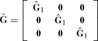
which is a 6 by 6 block diagonal matrix. Since the covariance structure for error is assumed to be spherical (σ²I), we do not need to specify this default choice in the SAS code. A REPEATED statement would be needed if any other covariance structure for error were to be specified. Under assumed sphericity, the estimated error variance is =3.3023.

The effects of the intercept and slope are in part fixed and in part random. These are represented as , where β₀ and β₁ are the fixed parameters and ν₀ and ν₁ are the random coefficients, in each case respectively for the INTERCEPT and slope for AGE. The estimate of β and the predicted values of the random effects ν are presented in two separate tables in Output 6.9. Specifically,

Also presented are the corresponding standard errors, the prediction errors, and corresponding tests for significance. It may be remarked that since ν_i′s are random rather than fixed parameters, hypothesis testing on them may not be meaningful.

EXAMPLE 9

Modeling Linear Growth, Ramus Heights Data To further illustrate the use of the random coefficients models, we will analyze the ramus heights data of Elston and Grizzle (1962) where the heights of the ramus bone (in mm) for 20 boys were measured at 8, 8, 9, and 9 years of age. We may want to model the ramus height, say y_t, at age t as a polynomial growth function of their ages. Since these boys are a sample from a hypothetical population of all boys, the modeled growth curve can be thought of as the common growth curve for the population. However, due to many genetic and environmental variations, each boy would have his own individual growth curve which can be thought of as a random variation of the population growth curve.

For a given boy, we consider the model

where ϵ_t~ N(0,σ²) are independent and the values of β₀ and β₁ are specific to the specific boy. In other words, β₀ and β₁ are random coefficients. It is possible that only one of the two coefficients may be random. For example, if β₀ is fixed and β₁ is random then all the boys will have the common intercept of the population but different rate of growth. The difference is modeled as β₁=β_1F +β_1R, where β_1F is the fixed common slope for the population and β_1R is the random part representing the amount of change from the common slope for the specific individual (boy). We assume E(β_1R)=0 and var(β_1R)=σ_β1². Similarly, if β₁ is fixed then all the boys will have the common rate of growth of the population but will have different intercepts. The appropriate assumptions to accommodate this case are β₀=β_0F+β_0R, where β_0F is the fixed common intercept for the population and β_0R is the random part representing the amount of change from the common intercept for the specific individual (boy). We assume E(β_0R)=0 and var(β_0R)=σ_β0². If both β₀ and β₁ are random then the above assumptions and interpretations hold for both coefficients. We will illustrate the case when only β₁ is random.

The SAS code is presented as Program 6.10. For the sake of completeness we have also added the code for the other two cases in the same program (but they have been commented out).

If only β₁ is random but β₀ is fixed then the model (6.18) results in

Thus β₀+β_1F age_t represents the fixed part of the model and β_1R is a normally distributed random coefficient with zero mean, and variance σ_β1². Thus, σ²G₁ is a 1 by 1 matrix, namely (σ_β1²). The errors ϵ_t are assumed to be independent and have a common variance, say, σ². That is, the spherical structure for the variance covariance matrix of the errors is assumed. Since , or equivalently, , the option TYPE=SIM for the covariance structure of G₁ can be used (in fact, this is a default option). Thus the appropriate MODEL and RANDOM statements are given by

model y=age/s;
random age/type=sim subject=boy;

where the option S in the MODEL statement requests that the solution for the fixed effects be printed. The option SUBJECT = BOY indicates that the observations on a given BOY constitute the vector of repeated measures. We have chosen to use the METHOD=REML option as the choice of estimation procedure. The complete code is given in Program 6.10. The corresponding output appears as Output 6.10.

/* Program 6.10 */

options ls = 64 ps=45 nodate nonumber;
    title1 'Output 6.10';
    title2 'Analysis of Ramus Data';
    data ramus;
    input boy y1 y2 y3 y4;
    y=y1;
    age=8;
    output;
    y=y2;
    age=8.5;
    output;
    y=y3;
    age=9;
    output;
    y=y4;
    age=9.5;
    output;
    lines;
    1 47.8 48.8 49.  49.7
    2 46.4 47.3 47.7 48.4
    3 46.3 46.8 47.8 48.5
    4 45.1 45.3 46.1 47.2
    5 47.6 48.5 48.9 49.3
    6 52.5 53.2 53.3 53.7
    7 51.2 53. 54.3 54.5

8 49.8 50. 50.3 52.7
    9 48.1 50.8 52.3 54.4
    10 45. 47. 47.3 48.3
    11 51.2 51.4 51.6 51.9
    12 48.5 49.2 53. 55.5
    13 52.1 52.8 53.7 55.
    14 48.2 48.9 49.3 49.8
    15 49.6 50.4 51.2 51.8
    16 50.7 51.7 52.7 53.3
    17 47.2 47.7 48.4 49.5
    18 53.3 54.6 55.1 55.3
    19 46.2 47.5 48.1 48.4
    20 46.3 47.6 51.0 51.8
    ;
    /* Source: Elston and Grizzle (1962).  Reproduced by
    permission of the International Biometric Society. */
    proc mixed data=ramus covtest;
    class boy;
    model y=age/s;
    random age /type = simple subject = boy;
    title3 'Only slope is random';
    run;
    /*
    proc mixed data=ramus covtest;
    class boy;
    model y=age/s;
    random int /type = simple subject = boy;
    title3 'Only intercept is random';
    run;
    proc mixed data=ramus covtest;
    class boy;
    model y=age/s;
    random int age /type = simple subject = boy;
    title3 'Both intercept and slope are random';
    run;
    */

Example 6.10. Output 6.10

Analysis of Ramus Data
                      Only slope is random

             Covariance Parameter Estimates (REML)

Cov Parm   Subject      Estimate     Std Error       Z  Pr > |Z|

AGE        BOY        0.07944986    0.02647746    3.00    0.0027
Residual              0.66113890    0.12172554    5.43    0.0001


                  Solution for Fixed Effects

 Effect         Estimate     Std Error    DF       t  Pr > |t|

 INTERCEPT   33.77000000    1.42583383    59   23.68    0.0001
 AGE          1.86300000    0.17440771    19   10.68    0.0001

Tests of Fixed Effects

           Source      NDF   DDF  Type III F  Pr > F

           AGE           1    19      114.10  0.0001

From Output 6.10 we find the estimates of variance components as =0.6611, =0.0794, and = = 0.0525. It is appropriate to test the null hypothesis H₀:σ_β1²=0 against the one-sided alternative. Testing H₀:σ_β1²=0 is equivalent to testing H₀: δ=0. Wald's test given in the output tests this null hypothesis against the two-sided alternative. The p value under the one-sided alternative can be computed as one-half of the reported p value. For our case, it is 0.0027/2≈ 0.0014, which is statistically significant. Thus we can claim σ_β1² to be nonzero. Since E(y_t)=β₀+β_1Fage_t, an estimate of average ramus height at time t is given by

Suppose instead of fitting Equation 6.9, we decide to fit Equation 6.18 with a 4 by 1 vector of ϵ_t for each subject having a compound symmetric (CS) structure. In this case, there are no random effects in the model given in Equation 6.18, but the covariance structure within each subject would need to be specified using the REPEATED statement

repeated/type=cs subject=boy r;

where SUBJECT=BOY indicates that repeated measures which are assumed to be independent are taken on boys. Option R in the REPEATED statement prints a typical diagonal block of the block diagonal matrix R. However, we will not discuss this model further here.