Day 12 OSPF Routing
CCNA 640-802 Exam Topics
![]() Configure, verify, and troubleshoot OSPF.
Configure, verify, and troubleshoot OSPF.
Key Topics
Open Shortest Path First (OSPF) is a link-state routing protocol that was developed as a replacement for Routing Information Protocol (RIP). OSPF’s major advantages over RIP are its fast convergence and its scalability to much larger network implementations. Today we review the operation, configuration, verification, and troubleshooting of basic OSPF.
OSPF Operation
IETF chose OSPF over Intermediate System-to-Intermediate System (IS-IS) as its recommended Interior Gateway Protocol (IGP). In 1998, the OSPFv2 specification was updated in RFC 2328 and is the current RFC for OSPF. RFC 2328, OSPF Version 2, is on the IETF website at http://www.ietf.org/rfc/rfc2328. Cisco IOS Software will choose OSPF routes over RIP routes because OSPF has an administrative distance of 110 versus RIP’s AD of 120.
OSPF Message Format
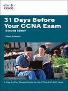
The data portion of an OSPF message is encapsulated in a packet. This data field can include one of five OSPF packet types. Figure 12-1 shows an encapsulated OSPF message in an Ethernet frame.

The OSPF packet header is included with every OSPF packet, regardless of its type. The OSPF packet header and packet type-specific data are then encapsulated in an IP packet. In the IP packet header, the protocol field is set to 89 to indicate OSPF, and the destination address is typically set to one of two multicast addresses: 224.0.0.5 or 224.0.0.6. If the OSPF packet is encapsulated in an Ethernet frame, the destination MAC address is also a multicast address: 01-00-5E-00-00-05 or 01-00-5E-00-00-06.
OSPF Packet Types
These five OSPF packet types each serve a specific purpose in the routing process:
![]() Hello:: Hello packets are used to establish and maintain adjacency with other OSPF routers.
Hello:: Hello packets are used to establish and maintain adjacency with other OSPF routers.
![]() DBD:: The database description (DBD) packet contains an abbreviated list of the sending router’s link-state database and is used by receiving routers to check against the local link-state database.
DBD:: The database description (DBD) packet contains an abbreviated list of the sending router’s link-state database and is used by receiving routers to check against the local link-state database.
![]() LSR:: Receiving routers can then request more information about any entry in the DBD by sending a link-state request (LSR).
LSR:: Receiving routers can then request more information about any entry in the DBD by sending a link-state request (LSR).
![]() LSU:: Link-state update (LSU) packets are used to reply to LSRs and to announce new information. LSUs contain 11 types of link-state advertisements (LSA).
LSU:: Link-state update (LSU) packets are used to reply to LSRs and to announce new information. LSUs contain 11 types of link-state advertisements (LSA).
![]() LSAck:: When an LSU is received, the router sends a link-state acknowledgment (LSAck) to confirm receipt of the LSU.
LSAck:: When an LSU is received, the router sends a link-state acknowledgment (LSAck) to confirm receipt of the LSU.
Neighbor Establishment
Hello packets are exchanged between OSPF neighbors to establish adjacency. Figure 12-2 shows the OSPF header and Hello packet.
Important fields shown in the figure include the following:
![]() Type:: OSPF packet type: Hello (Type 1), DBD (Type 2), LS Request (Type 3), LS Update (Type 4), LS ACK (Type 5)
Type:: OSPF packet type: Hello (Type 1), DBD (Type 2), LS Request (Type 3), LS Update (Type 4), LS ACK (Type 5)
![]() Router ID:: ID of the originating router
Router ID:: ID of the originating router
![]() Area ID:: Area from which the packet originated
Area ID:: Area from which the packet originated
![]() Network Mask:: Subnet mask associated with the sending interface
Network Mask:: Subnet mask associated with the sending interface
![]() Hello Interval:: Number of seconds between the sending router’s Hellos
Hello Interval:: Number of seconds between the sending router’s Hellos
![]() Router Priority:: Used in DR/BDR election (discussed later in the section “DR/BDR Election”)
Router Priority:: Used in DR/BDR election (discussed later in the section “DR/BDR Election”)
![]() Designated Router (DR):: Router ID of the DR, if any
Designated Router (DR):: Router ID of the DR, if any
![]() Backup Designated Router (BDR):: Router ID of the BDR, if any
Backup Designated Router (BDR):: Router ID of the BDR, if any
![]() List of Neighbors:: Lists the OSPF Router ID of the neighboring router(s)
List of Neighbors:: Lists the OSPF Router ID of the neighboring router(s)
Hello packets are used to do the following:
![]() Discover OSPF neighbors and establish neighbor adjacencies
Discover OSPF neighbors and establish neighbor adjacencies
![]() Advertise parameters on which two routers must agree to become neighbors
Advertise parameters on which two routers must agree to become neighbors
![]() Elect the DR and BDR on multiaccess networks such as Ethernet and Frame Relay
Elect the DR and BDR on multiaccess networks such as Ethernet and Frame Relay
Receiving an OSPF Hello packet on an interface confirms for a router that another OSPF router exists on this link. OSPF then establishes adjacency with the neighbor. To establish adjacency, two OSPF routers must have the following matching interface values:
![]() Hello Interval
Hello Interval
![]() Dead Interval
Dead Interval
![]() Network Type
Network Type
![]() Area ID
Area ID
Before both routers can establish adjacency, both interfaces must be part of the same network, including the same subnet mask. Then full adjacency will happen after both routers have exchanged any necessary LSUs and have identical link-state databases. By default, OSPF Hello packets are sent to the multicast address 224.0.0.5 (ALLSPFRouters) every 10 seconds on multiaccess and point-to-point segments and every 30 seconds on nonbroadcast multiaccess (NBMA) segments (Frame Relay, X.25, ATM). The default dead interval is four times the Hello interval.
Link-State Advertisements
Link-state updates (LSUs) are the packets used for OSPF routing updates. An LSU packet can contain 11 types of link-state advertisements (LSAs), as shown in Figure 12-3.

OSPF Network Types
OSPF defines five network types:
![]() Point-to-point
Point-to-point
![]() Broadcast multiaccess
Broadcast multiaccess
![]() Nonbroadcast multiaccess
Nonbroadcast multiaccess
![]() Point-to-multipoint
Point-to-multipoint
![]() Virtual links
Virtual links
Multiaccess networks create two challenges for OSPF regarding the flooding of LSAs:
![]() Creation of multiple adjacencies, one adjacency for every pair of routers
Creation of multiple adjacencies, one adjacency for every pair of routers
![]() Extensive flooding of LSAs
Extensive flooding of LSAs
DR/BDR Election
The solution to managing the number of adjacencies and the flooding of LSAs on a multiaccess network is the designated router (DR). To reduce the amount of OSPF traffic on multiaccess networks, OSPF elects a DR and backup DR (BDR). The DR is responsible for updating all other OSPF routers when a change occurs in the multiaccess network. The BDR monitors the DR and takes over as DR if the current DR fails.
The following criteria is used to elect the DR and BDR:
-
DR: Router with the highest OSPF interface priority.
-
BDR: Router with the second highest OSPF interface priority.
-
If OSPF interface priorities are equal, the highest router ID is used to break the tie.
When the DR is elected, it remains the DR until one of the following conditions occurs:
![]() The DR fails.
The DR fails.
![]() The OSPF process on the DR fails.
The OSPF process on the DR fails.
![]() The multiaccess interface on the DR fails.
The multiaccess interface on the DR fails.
If the DR fails, the BDR assumes the role of DR, and an election is held to choose a new BDR. If a new router enters the network after the DR and BDR have been elected, it will not become the DR or the BDR even if it has a higher OSPF interface priority or router ID than the current DR or BDR. The new router can be elected the BDR if the current DR or BDR fails. If the current DR fails, the BDR will become the DR, and the new router can be elected the new BDR.
Without additional configuration, you can control the routers that win the DR and BDR elections by doing either of the following:
![]() Boot the DR first, followed by the BDR, and then boot all other routers.
Boot the DR first, followed by the BDR, and then boot all other routers.
![]() Shut down the interface on all routers, followed by a no shutdown on the DR, then the BDR, and then all other routers.
Shut down the interface on all routers, followed by a no shutdown on the DR, then the BDR, and then all other routers.
However, the recommended way to control DR/BDR elections is to change the interface priority, which we review in the “OSPF Configuration” section.
OSPF Algorithm
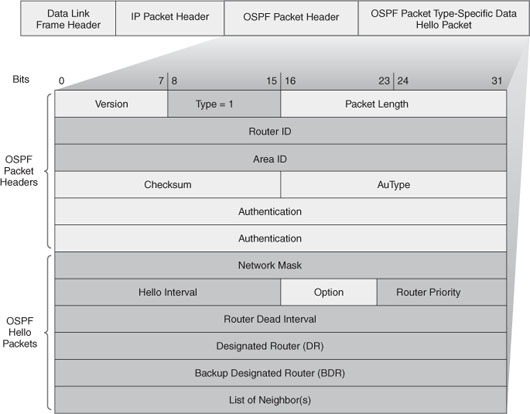
Each OSPF router maintains a link-state database containing the LSAs received from all other routers. When a router has received all the LSAs and built its local link-state database, OSPF uses Dijkstra’s shortest path first (SPF) algorithm to create an SPF tree. This algorithm accumulates costs along each path, from source to destination. The SPF tree is then used to populate the IP routing table with the best paths to each network.
For example, in Figure 12-4 each path is labeled with an arbitrary value for cost. The cost of the shortest path for R2 to send packets to the LAN attached to R3 is 27 (20 + 5 + 2 = 27). Notice that this cost is not 27 for all routers to reach the LAN attached to R3. Each router determines its own cost to each destination in the topology. In other words, each router uses the SPF algorithm to calculate the cost of each path to a network and determines the best path to that network from its own perspective.
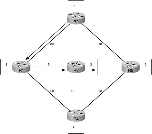
Table 12-1 lists, for R1, the shortest path to each LAN, along with the cost.

You should be able to create a similar table for each of the other routers in Figure 12-4.
Link-State Routing Process
The following list summarizes the link-state routing process used by OSPF. All OSPF routers complete the following generic link-state routing process to reach a state of convergence:
-
Each router learns about its own links, and its own directly connected networks. This is done by detecting that an interface is in the up state, including a Layer 3 address.
-
Each router is responsible for establishing adjacency with its neighbors on directly connected networks by exchanging Hello packets.
-
Each router builds a link-state packet (LSP) containing the state of each directly connected link. This is done by recording all the pertinent information about each neighbor, including neighbor ID, link type, and bandwidth.
-
Each router floods the LSP to all neighbors, who then store all LSPs received in a database. Neighbors then flood the LSPs to their neighbors until all routers in the area have received the LSPs. Each router stores a copy of each LSP received from its neighbors in a local database.
-
Each router uses the database to construct a complete map of the topology and computes the best path to each destination network. The SPF algorithm is used to construct the map of the topology and to determine the best path to each network. All routers will have a common map or tree of the topology, but each router independently determines the best path to each network within that topology.
OSPF Configuration
To review the OSPF configuration commands, we will use the topology in Figure 12-5 and the addressing scheme in Table 12-2.


The router ospf Command
OSPF is enabled with the router ospf process-id global configuration command:
R1(config)#router ospf 1
The process-id is a number between 1 and 65,535 and is chosen by the network administrator. The process ID is locally significant. It does not have to match other OSPF routers to establish adjacencies with those neighbors. This differs from EIGRP. The EIGRP process ID or autonomous system number must match before two EIGRP neighbors will become adjacent.
For our review, we will enable OSPF on all three routers using the same process ID of 1.
The network Command
The network command is used in router configuration mode:
Router(config-router)#network network-address wildcard-mask area area-id
The OSPF network command uses a combination of network-address and wildcard-mask. The network address, along with the wildcard mask, is used to specify the interface or range of interfaces that will be enabled for OSPF using this network command.
The wildcard mask is customarily configured as the inverse of a subnet mask. For example, R1’s FastEthernet 0/0 interface is on the 172.16.1.16/28 network. The subnet mask for this interface is /28 or 255.255.255.240. The inverse of the subnet mask results in the wildcard mask 0.0.0.15.
The area area-id refers to the OSPF area. An OSPF area is a group of routers that share link-state information. All OSPF routers in the same area must have the same link-state information in their link-state databases. Therefore, all the routers within the same OSPF area must be configured with the same area ID on all routers. By convention, the area ID is 0.
Example 12-1 shows the network commands for all three routers, enabling OSPF on all interfaces.
Example 12-1 Configuring OSPF Networks
R1(config)#router ospf 1
R1(config-router)#network 172.16.1.16 0.0.0.15 area 0
R1(config-router)#network 192.168.10.0 0.0.0.3 area 0
R1(config-router)#network 192.168.10.4 0.0.0.3 area 0
_____________________________________________________
R2(config)#router ospf 1
R2(config-router)#network 10.10.10.0 0.0.0.255 area 0
R2(config-router)#network 192.168.10.0 0.0.0.3 area 0
R2(config-router)#network 192.168.10.8 0.0.0.3 area 0
_____________________________________________________
R3(config)#router ospf 1
R3(config-router)#network 172.16.1.32 0.0.0.7 area 0
R3(config-router)#network 192.168.10.4 0.0.0.3 area 0
R3(config-router)#network 192.168.10.8 0.0.0.3 area 0
Router ID
The router ID plays an important role in OSPF. It is used to uniquely identify each router in the OSPF routing domain. Cisco routers derive the router ID based on three criteria in the following order:
-
Use the IP address configured with the OSPF router-id command.
-
If the router ID is not configured, the router chooses the highest IP address of any of its loopback interfaces.
-
If no loopback interfaces are configured, the router chooses the highest active IP address of any of its physical interfaces.
The router ID can be viewed with several commands including show ip ospf interfaces, show ip protocols, and show ip ospf.
Two ways to influence the router ID are to configure a loopback address or configure the router ID. The advantage of using a loopback interface is that, unlike physical interfaces, it cannot fail. Therefore, using a loopback address for the router ID provides stability to the OSPF process.
Because the OSPF router-id command is a fairly recent addition to Cisco IOS Software (Release 12.0[1]T), it is more common to find loopback addresses used for configuring OSPF router IDs.
Example 12-2 shows the loopback configurations for the routers in our topology.
Example 12-2 Loopback Configurations
R1(config)#interface loopback 0
R1(config-if)#ip address 10.1.1.1 255.255.255.255
_________________________________________________
R2(config)#interface loopback 0
R2(config-if)#ip address 10.2.2.2 255.255.255.255
_________________________________________________
R3(config)#interface loopback 0
R3(config-if)#ip address 10.3.3.3 255.255.255.255
To configure the router ID, use the following command syntax:
Router(config)#router ospf process-id
Router(config-router)#router-id ip-address
The router ID is selected when OSPF is configured with its first OSPF network command. So the loopback or router ID command should already be configured. However, you can force OSPF to release its current ID and use the loopback or configured router ID by either reloading the router or using the following command:
Router#clear ip ospf process
Modifying the OSPF Metric
Cisco IOS Software uses the cumulative bandwidths of the outgoing interfaces from the router to the destination network as the cost value. At each router, the cost for an interface is calculated using the following formula:
Cisco IOS Cost for OSPF = 108/bandwidth in bps
In this calculation, the value 108 is known as the reference bandwidth. The reference bandwidth can be modified to accommodate networks with links faster than 100,000,000 bps (100 Mbps) using the OSPF command auto-cost reference-bandwidth interface command. When used, this command should be entered on all routers so that the OSPF routing metric remains consistent. Table 12-3 shows the default OSPF costs using the default reference bandwidth for several types of interfaces.

You can modify the OSPF metric in two ways:
![]() Use the bandwidth command to modify the bandwidth value used by the Cisco IOS Software in calculating the OSPF cost metric.
Use the bandwidth command to modify the bandwidth value used by the Cisco IOS Software in calculating the OSPF cost metric.
![]() Use the ip ospf cost command, which allows you to directly specify the cost of an interface.
Use the ip ospf cost command, which allows you to directly specify the cost of an interface.
Table 12-4 shows the two alternatives that can be used in modifying the costs of the serial links in the topology. The right side shows the ip ospf cost command equivalents of the bandwidth commands on the left.

Controlling the DR/BDR Election
Because the DR becomes the focal point for the collection and distribution of LSAs in a multiaccess network, it is important for this router to have sufficient CPU and memory capacity to handle the responsibility. Instead of relying on the router ID to decide which routers are elected the DR and BDR, it is better to control the election of these routers with the ip ospf priority interface command:
Router(config-if)#ip ospf priority {0 - 255}
The priority value defaults to 1 for all router interfaces, which means the router ID determines the DR and BDR. If you change the default value from 1 to a higher value, however, the router with the highest priority becomes the DR, and the router with the next highest priority becomes the BDR. A value of 0 makes the router ineligible to become a DR or BDR.
All the routers in Figure 12-6 booted at the same time with a complete OSPF configuration. In such a situation, RouterC is elected the DR, and RouterB is elected the BDR based on the highest router IDs.

Let’s assume RouterA is the better candidate to be DR and RouterB should be BDR. However, you do not want to change the addressing scheme. Example 12-3 shows a way to control the DR/BDR election in the topology shown in Figure 12-6.
Notice we changed both routers. Although RouterB was the BDR without doing anything, it would lose this role to RouterC if we did not configure RouterB’s priority to be higher than the default.
Redistributing a Default Route
Returning to the first topology shown in Figure 12-5, we can simulate a connection to the Internet on R1 by configuring a loopback interface. R1 is now called an Autonomous System Boundary Router (ASBR). Then we can redistribute the default static route to R2 and R3 with the default-information originate command, as demonstrated in Example 12-4.
Modifying Hello Intervals and Hold Times
It might be desirable to change the OSPF timers so that routers will detect network failures in less time. Doing this will increase traffic, but sometimes there is a need for quick convergence that outweighs the extra traffic.
OSPF Hello and Dead intervals can be modified manually using the following interface commands:
Router(config-if)#ip ospf hello-interval seconds
Router(config-if)#ip ospf dead-interval seconds
Example 12-5 shows the Hello and Dead intervals modified to 5 seconds and 20 seconds, respectively, on the Serial 0/0/0 interface for R1.
Remember, unlike EIGRP, OSPF Hello and Dead intervals must be equivalent between neighbors. So R2 should be configured with the same intervals.
Verifying and Troubleshooting OSPF
To verify any routing configuration, you will most likely depend on the show ip route, show ip interface brief, and show ip protocols commands. The routing table should have all the expected routes. If not, check the status of all interfaces to ensure that an interface is not down or misconfigured. For our example, the routing tables for OSPF will have an O*E2 route on R2 and R3 as shown in R2’s routing table in Example 12-6.
OSPF external routes fall into one of two categories:
![]() External Type 1 (E1):: OSPF accumulates cost for an E1 route as the route is being propagated throughout the OSPF area.
External Type 1 (E1):: OSPF accumulates cost for an E1 route as the route is being propagated throughout the OSPF area.
![]() External Type 2 (E2):: The cost of an E2 route is always the external cost, irrespective of the interior cost to reach that route.
External Type 2 (E2):: The cost of an E2 route is always the external cost, irrespective of the interior cost to reach that route.
In this topology, because the default route has an external cost of 1 on the R1 router, R2 and R3 also show a cost of 1 for the default E2 route. E2 routes at a cost of 1 are the default OSPF configuration.
You can verify that expected neighbors have established adjacency with the show ip ospf neighbor command. Example 12-7 shows the neighbor tables for all three routers.

For each neighbor, this command displays the following output:
![]() Neighbor ID:: The router ID of the neighboring router.
Neighbor ID:: The router ID of the neighboring router.
![]() Pri:: The OSPF priority of the interface. These all show 0 because point-to-point links do not elect a DR or BDR.
Pri:: The OSPF priority of the interface. These all show 0 because point-to-point links do not elect a DR or BDR.
![]() State:: The OSPF state of the interface. FULL state means that the router’s interface is fully adjacent with its neighbor and they have identical OSPF link-state databases.
State:: The OSPF state of the interface. FULL state means that the router’s interface is fully adjacent with its neighbor and they have identical OSPF link-state databases.
![]() Dead Time:: The amount of time remaining that the router will wait to receive an OSPF Hello packet from the neighbor before declaring the neighbor down. This value is reset when the interface receives a Hello packet.
Dead Time:: The amount of time remaining that the router will wait to receive an OSPF Hello packet from the neighbor before declaring the neighbor down. This value is reset when the interface receives a Hello packet.
![]() Address:: The IP address of the neighbor’s interface to which this router is directly connected.
Address:: The IP address of the neighbor’s interface to which this router is directly connected.
![]() Interface:: The interface on which this router has formed adjacency with the neighbor.
Interface:: The interface on which this router has formed adjacency with the neighbor.
As shown in Example 12-8, you can use the show ip protocols command as a quick way to verify vital OSPF configuration information, including the OSPF process ID, the router ID, networks the router is advertising, the neighbors from which the router is receiving updates, and the default AD, which is 110 for OSPF.

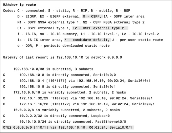
The show ip ospf command shown in Example 12-9 for R2 can also be used to examine the OSPF process ID and router ID. In addition, this command displays the OSPF area information and the last time the SPF algorithm was calculated.
Example 12-9 The show ip ospf Command
R2#show ip ospf
Routing Process "ospf 1" with ID 10.2.2.2
Supports only single TOS(TOS0) routes
Supports opaque LSA
Supports Link-local Signaling (LLS)
Supports area transit capability
Initial SPF schedule delay 5000 msecs
Minimum hold time between two consecutive SPFs 10000 msecs
Maximum wait time between two consecutive SPFs 10000 msecs
Incremental-SPF disabled
Minimum LSA interval 5 secs
Minimum LSA arrival 1000 msecs
LSA group pacing timer 240 secs
Interface flood pacing timer 33 msecs
Retransmission pacing timer 66 msecs
Number of external LSA 1. Checksum Sum 0x0025BD
Number of opaque AS LSA 0. Checksum Sum 0x000000
Number of DCbitless external and opaque AS LSA 0
Number of DoNotAge external and opaque AS LSA 0
Number of areas in this router is 1. 1 normal 0 stub 0 nssa
Number of areas transit capable is 0
External flood list length 0
IETF NSF helper support enabled
Cisco NSF helper support enabled
Area BACKBONE(0)
Number of interfaces in this area is 3
Area has no authentication
SPF algorithm last executed 02:09:55.060 ago
SPF algorithm executed 4 times
Area ranges are
Number of LSA 3. Checksum Sum 0x013AB0
Number of opaque link LSA 0. Checksum Sum 0x000000
Number of DCbitless LSA 0
Number of indication LSA 0
Number of DoNotAge LSA 0
Flood list length 0
The quickest way to verify Hello and Dead intervals is to use the show ip ospf interface command. As shown in Example 12-10 for R2, adding the interface name and number to the command displays output for a specific interface.
Example 12-10 The show ip ospf interface Command
R2#show ip ospf interface serial 0/0/0
Serial0/0/0 is up, line protocol is up
Internet Address 192.168.10.2/30, Area 0
Process ID 1, Router ID 10.2.2.2, Network Type POINT_TO_POINT, Cost: 1562
Transmit Delay is 1 sec, State POINT_TO_POINT
Timer intervals configured, Hello 5, Dead 20, Wait 20, Retransmit 5
oob-resync timeout 40
Hello due in 00:00:03
Supports Link-local Signaling (LLS)
Cisco NSF helper support enabled
IETF NSF helper support enabled
Index 1/1, flood queue length 0
Next 0x0(0)/0x0(0)
Last flood scan length is 1, maximum is 1
Last flood scan time is 0 msec, maximum is 0 msec
Neighbor Count is 1, Adjacent neighbor count is 1
Adjacent with neighbor 172.30.1.1
Suppress hello for 0 neighbor(s)
As highlighted in Example 12-10, the show ip ospf interface command also shows you the router ID, network type, and the cost for the link, as well as the neighbor to which this interface is adjacent.