3.3. Multiple-precision Integer Arithmetic

Cryptographic protocols based on the rings and demand n and p to be sufficiently large (of bit length ≥ 512) in order to achieve the desired level of security. However, standard compilers do not support data types to hold with full precision the integers of this size. For example, C compilers support integers of size ≤ 64 bits. So one must employ custom-designed data types for representing and working with such big integers. Many libraries are already available that can handle integers of arbitrary length. FREELIP, GMP, LiDIA, NTL and ZEN are some such libraries that are even freely available.

Alternatively, one may design one’s own functions for multiple-precision integers. Such a programming exercise is not very difficult, but making the functions run efficiently is a huge challenge. Several tricks and optimization techniques can turn a naive implementation to a much faster and more memory-efficient code and it needs years of experimental experience to find out the subtleties. Theoretical asymptotic estimates might serve as a guideline, but only experimentation can settle the relative merits and demerits of the available algorithms for input sizes of practical interest. For example, the theoretically fastest algorithm known for multiplying two multiple-precision integers is based on the so-called fast Fourier transform (FFT) techniques. But our experience shows that this algorithm starts to outperform other common but asymptotically slower algorithms only when the input size is at least several thousand bits. Since such very large integers are rarely needed by cryptographic protocols, FFT-based multiplication is not useful in this context.

3.3.1. Representation of Large Integers

In order to represent a large integer, we break it up into small parts and store each part in a memory word^[3] accessible by built-in data types. The simplest way to break up a (positive) integer a is to predetermine a radix ℜ and compute the ℜ-ary representation (a_s–1, . . . , a₀)_ℜ of a (see Exercise 3.8). One should have ℜ ≤ 2³² so that each ℜ-ary digit a_i can be stored in a memory word. For the sake of efficiency, it is advisable to take ℜ to be a power of 2. It is also expedient to take ℜ as large as possible, because smaller values of ℜ lead to (possibly) longer size s and thereby add to the storage requirement and also to the running time of arithmetic functions. The best choice is ℜ = 2³². We denote by ulong a built-in unsigned integer data type provided by the compiler (like the ANSI C standard unsigned long). We use an array of ulong for storing the digits. The array can be static or dynamic. Though dynamic arrays are more storage-efficient (because they can be allocated only as much memory as needed), they have memory allocation and deallocation overheads and are somewhat more complicated to programme than static arrays. Moreover, for cryptographic protocols one typically needs integers no longer than 4096 bits. Since the product of two integers of bit size t has bit size ≤ 2t, a static array of 8192/32 = 256 ulong suffices for storing cryptographic integers. It is also necessary to keep track of the actual size of an integer, since filling up with leading 0 digits is not an efficient strategy. Finally, it is often useful to have a signed representation of integers. A sign bit is also necessary for this case. We state three possible declarations in Exercise 3.11.

^[3] We assume that a word in the memory is 32 bits long.

3.3.2. Basic Arithmetic Operations

We now describe the implementations of addition, subtraction, multiplication and Euclidean division of multiple-precision integers. Every other complex operation (like modular arithmetic, gcd) is based on these primitives. It is, therefore, of utmost importance to write efficient codes for these basic operations.

For integers of cryptographic sizes, the most efficient algorithms are the standard ones we use for doing arithmetic on decimal numbers, that is, for two positive integers a = a_s–1 . . . a₀ and b = b_t–1 . . . b₀ we compute the sum c = a + b = c_r–1 . . . c₀ as follows. We first compute a₀ + b₀. If this sum is ≥ ℜ, then c₀ = a₀ + b₀ – ℜ and the carry is 1, otherwise c₀ = a₀ + b₀ and the carry is 0. We then compute a₁ + b₁ plus the carry available from the previous digit, and compute c₁ and the next carry as before.

For computing the product d = ab = d_l–1 . . . d₀, we do the usual quadratic procedure; namely, we initialize all the digits of d to 0 and for each i = 0, . . . , s – 1 and j = 0, . . . , t – 1 we compute a_ib_j and add it to the (i + j)-th digit of d. If this sum (call it σ) at the (i + j)-th location exceeds ℜ – 1, we find out q, r with σ = qℜ + r, r < ℜ. Then d_i+j is assigned r, and q is added to the (i + j + 1)-st location. If that addition results in a carry, we propagate the carry to higher locations until it gets fully absorbed in some word of d.

All these sound simple, but complications arise when we consider the fact that the sum of two 32-bit words (and a possible carry from the previous location) may be 33 bits long. For multiplication, the situation is even worse, because the product a_ib_j can be 64 bits long. Since our machine word can hold only 32 bits, it becomes problematic to hold all these intermediate sums and products to full precision. We assume that the least significant 32 bits are correctly returned and assigned to the output variable (ulong), whereas the leading 32 bits are lost.^[4] The most efficient way to keep track of these overflows is to use assembly instructions and this is what many number theory packages (like PARI and UBASIC) do. But this means that for every target architecture we have to write different assembly codes. Here we describe certain tricks that make it possible to grab the overflow information with only high-level languages, without sufficiently degrading the performance compared to assembly instructions.

^[4] This is the typical behaviour of a CPU that supports 2’s complement arithmetic.

Addition and subtraction

First consider the sum a_i + b_i. We compute the least significant 32 bits by assigning c_i = a_i + b_i. It is easy to see that an overflow occurs during this sum if and only if c_i < a_i. We set the output carry accordingly. Now, let us consider the situation when we have an input carry: that is, when we compute the sum c_i = a_i + b_i+1. Here an overflow occurs if and only if c_i ≤ a_i. Algorithm 3.1 performs this addition of words.

Algorithm 3.1. Addition of words

Input: Words ai and bi and the input carry . Output: Word ci and the output carry with ai + bi + γi = ci + δiℜ. Steps: ci := ai + bi. if (γi) { ci ++, δi := ( (ci ≤ ai) ? 1 : 0 ). } else { δi := ( (ci < ai) ? 1 : 0 ). }

Algorithm 3.1 assumes that c_i and a_i are stored in different memory words. If this is not the case, we should store a_i + b_i in a temporary variable and, after the second line, c_i should be assigned the value of this temporary variable. Note also that many processors provide an increment primitive which is faster than the general addition primitive. In that case, the statement c_i++ is preferable to c_i := c_i+1.

For subtraction, we proceed analogously from right to left and keep track of the borrow. Here the check for overflow can be done before the subtraction of words is carried out (and, therefore, no temporary variable is needed, if we assume that the output carry is not stored in the location of the operands).

Algorithm 3.2. Subtraction of words

Input: Words ai and bi and the input borrow . Output: Word ci and the output borrow with ai – bi – γi = ci – δiℜ. Steps: if (γi) { δi := ( (ai ≤ bi) ? 1 : 0 ), ci := ai – bi, ci – –. } else { δi := ( (ai < bi) ? 1 : 0 ), ci := ai – bi. }

We urge the reader to develop the complete addition and subtraction procedures for multiple-precision integers, based on the above primitives for words.

Multiplication

The product of two 32-bit words can be as long as 64 bits, and we plan to (compute and) store this product in two words. Assuming the availability of a built-in 64-bit unsigned integer data type (which we will henceforth denote as ullong), this can be performed as in Algorithm 3.3.

Algorithm 3.3. Multiplication of words

Input: Words a and b. Output: Words c and d with ab = cℜ + d. Steps: /* We use a temporary variable t of data type ullong */ t := (ullong)(a) * (ullong)(b), c := (ulong)(t ≫ 32), d := (ulong)t.

We use a temporary 64-bit integer variable t to store the product ab. The lower 32 bits of t is stored in d by simply typecasting, whereas the higher 32 bits of t is obtained by right-shifting t (the operator ≫) by 32 bits. This is a reasonable strategy given that we do not explore assembly-level instructions. Algorithm 3.4 describes a multiplication algorithm for two multiple-precision integer operands, that does not directly use the word-multiplying primitive of Algorithm 3.3.

The reader can verify easily that this code properly computes the product. We now highlight how this makes the computation efficient. The intermediate results are stored in the array t of 64-bit ullong. This means that after the 64-bit product a_ib_j of words a_i and b_j is computed (in the temporary variable T), we directly add T to the location t_i+j. If the sum exceeds ℜ² – 1 = 2⁶⁴ – 1, that is, if an overflow occurs, we should add ℜ to t_{i + j + 1} or equivalently 1 to t_i+j+2. This last addition is one of ullong integers and can be made more efficient, if this is replaced by ulong increments, and this is what we do using the temporary array u. Since the quadratic loop is the bottleneck of the multiplication procedure, it is absolutely necessary to make this loop as efficient as possible.

Algorithm 3.4. Multiplication of multiple-precision integers

Input: Integers a = (ar–1 . . . a0)ℜ and b = (bs–1 . . . b0)ℜ Output: The product c = (cr+s–1 . . . c0)ℜ = ab. Steps: /* Let T be a variable and t0, . . . , tr+s–1 an array of ullong variables */ /* Let v be a variable and u0, . . . , ur+s–1 an array of ulong variables */ Initialize the array locations ci, ti and ui to 0 for all i = 0, . . . , r + s – 1. /* The quadratic loop */ for (i = 0, . . . , r – 1) and (j = 0, . . . , s – 1) {    T := (ullong)(ai) * (ullong)(bj).    if ((ti+j + = T) < T) ui+j+2 ++. } /* Deferred normalization */ for (i = 0, . . . , r + s – 1) {     if ((ci + = ui) < ui) ui+1 ++.     v := (ulong)(ti), if ((ci + = v) < v) ui+1++.     v := (ulong)(ti ≫ 32), if ((ci+1 + = v) < v) ui+2 ++. }

After the quadratic loop, we do deferred normalization from the array of 64-bit double-words t_i to the array of 32-bit words c_i. This is done using the typecasting and right-shift strategy mentioned in Algorithm 3.3. We should also take care of the intermediate carries stored in the array u. The normalization loop takes a total time of O(r + s), whereas the quadratic loop takes time O(rs). If we had done normalization inside the quadratic loop itself, that would incur an additional O(rs) cost (which is significantly more than that of deferred normalization).

Squaring

If both the operands a and b of multiplication are same, it is not necessary to compute a_ib_j and a_jb_i separately. We should add to t_i+j the product , if i = j, or the product 2a_ia_j, if i < j. Note that 2a_ia_j can be computed by left shifting a_ia_j by one bit. This might result in an overflow which can be checked before shifting by looking at the 64th bit of a_ia_j. Algorithm 3.5 incorporates these changes.

Fast multiplication

For the multiplication of two multiple-precision integers, there are algorithms that are asymptotically faster than the quadratic Algorithms 3.4 and 3.5. However, not all these theoretically faster algorithms are practical for sizes of integers used in cryptology. Our practical experience shows that a strategy due to Karatsuba outperforms the quadratic algorithm, if both the operands are of roughly equal sizes and if the bit lengths of the operands are 300 or more. We describe Karatsuba’s algorithm in connection with squaring, where the two operands are same (and hence of the same size). Suppose we want to compute a² for a multiple-precision integer a = (a_r–1 . . . a₀)_ℜ. We first break a into two integers of almost equal sizes, namely, α := (a_r–1 . . . a_t)_ℜ and β := (a_t–1 . . . a₀)_ℜ, so that a = ℜ^tα + β. Now, a² = α²ℜ^2t + 2αβℜ^t + β² and 2αβ = (α² + β²) – (α – β)². We recursively invoke Karatsuba’s multiplication with operands α, β and α – β. Recursion continues as long as the operands are not too small and the depth of recursion is within a prescribed limit. One can check that Karatsuba’s algorithm runs in time O(r^{lg 3} lg r) = O(r^1.585 lg r) which is a definite improvement over the O(r²) running time taken by the quadratic algorithm.

Algorithm 3.5. The quadratic loop for squaring

for (i = 0, . . . , r – 1) and (j = i, . . . , r – 1) {    T := (ullong)(ai) * (ullong)(aj).    if (i ≠ j) {       if (the 64th bit of T is 1) ui+j+2 ++.       T ≪= 1.    }    if ((ti+j + = T) < T) ui+j+2 ++. }

The best-known algorithm for multiplication of two multiple-precision integers is based on the fast Fourier transform (FFT) techniques and has running time O^~(r). However, for integers used in cryptology this algorithm is usually not practical. Therefore, we will not discuss FFT multiplication in this book.

Division

Euclidean division with remainder of multiple-precision integers is somewhat cumbersome, although conceptually as difficult (that is, as simple) as the division procedure of decimal integers, taught in early days of school. The most challenging part in the procedure is guessing the next digit in the quotient. For decimal integers, we usually do this by looking at the first few (decimal) digits of the divisor and the dividend. This need not give us the correct digit, but something close to the same. In the case of ℜ-ary digits, we also make a guess of the quotient digit based on a few leading ℜ-ary digits of the divisor and the dividend, but certain precautions have to be taken to ensure that the guess is not too different from the correct one.

Suppose we are given positive integers a = (a_r–1 . . . a₀)_ℜ and b = (b_s–1 . . . b₀)ℜ with a_r–1 ≠ 0 and b_s–1 ≠ 0, and we want to compute the integers x = (x_r–s . . . x₀)_ℜ and y = (y_s–1 . . . y₀)_ℜ with a = xb + y, 0 ≤ y < b. First, we want that b_s–1 ≥ ℜ/2 (you’ll see why, later). If this condition is already not met, we force it by multiplying both a and b by 2^t for some suitable t, 0 < t < 32. In that case, the quotient remains the same, but the remainder gets multiplied by 2^t. The desired remainder can be later found out easily by right-shifting the computed remainder by t bits. The process of making b_s–1 ≥ ℜ/2 is often called normalization (of b). Henceforth, we will assume that b is normalized. Note that normalization may increase the word-size of a by 1.

Algorithm 3.6. Euclidean division of multiple-precision integers

Input: Integers a = (ar–1 . . . a0)ℜ and b = (bs–1 . . . b0)ℜ with r ≥ 3, s ≥ 2, ar–1 ≠ 0, bs–1 ≥ ℜ/2 and a ≥ b. Output: The quotient x = (xr–s . . . x0)ℜ = a quot b and the remainder y = (ys–1 . . . y0)ℜ = a rem b of Euclidean division of a by b. Steps: Initialize the quotient digits xi to 0 for i = 0, . . . , r – s. /* The main loop */ for (i = r – 1, . . . , s) {    /* Initial check */    if (ai ≥ bs–1) and (a ≥ bℜi–s+1) { xi–s+1++, a := a – bℜi–s+1. }    /* Guess the next digit of quotient */    if (ai = bs–1) xi–s := ℜ – 1, else xi–s := ⌊(aiℜ + ai–1)/bs–1)⌋.    if (xi–s ≠ 0)        while (xi–s(bs–1ℜ + bs–2) > aiℜ2 + ai–1ℜ + ai–2) xi–s– –.    /* Modify the guess to the correct value */    z := xi–sbℜi–s.    if (a < z) { xi–s– –, z := z – bℜi–s. }    a := a – z. } /* Here the quotient may be one less than the actual value */ if (a ≥ b) { a := a – b, x := x+1. } y := a.

Algorithm 3.6 implements multiple-precision division. It is not difficult to prove the correctness of the algorithm. We refrain from doing so, but make some useful comments. The initial check inside the main loop may cause the increment of x_i–s+1. This may lead to a carry which has to be adjusted to higher digits. This carry propagation is not mentioned in the code for simplicity. Since b is assumed to be normalized, this initial check needs to be carried out only once; that is, for a non-normalized b we have to replace the if statement by a while loop. This is the first advantage of normalization. In the first step of guessing the quotient digit x_i–s, we compute ⌊(a_iℜ + a_i–1)/b_s–1⌋ using ullong arithmetic. At this point, the guess is based only on two leading digits of a and one leading digit of b. In the while loop, we refine this guess by considering one more digit of a and b each. Since b is normalized, this while loop is executed no more than twice (the second advantage of normalization). The guess for x_i–s made in this way is either equal to or one more than the correct value which is then computed by comparing a with x_i–sbℜ^i–s. The running time of the algorithm is O(s(r – s)). For a fixed r, this is maximum (namely O(r²)) when s ≈ r/2.

Bit-wise operations

Multiplication and division by a power of 2 can be carried out more efficiently using bit operations (on words) instead of calling the general procedures just described. It is also often necessary to compute the bit length of a non-zero multiple-precision integer and the multiplicity of 2 in it. In these cases also, one should use bit operations for efficiency. For these implementations, it is advantageous to maintain precomputed tables of the constants 2ⁱ, i = 0, . . . , 31, and of 2ⁱ – 1, i = 0, . . . , 32, rather than computing them in situ every time they are needed. In Algorithm 3.7, we describe an implementation of multiplication by a power of 2 (that is, the left shift operation). We use the symbols OR, ≫ and ≪ to denote bit-wise or, right shift and left shift operations on 32-bit integers.

Algorithm 3.7. Left-shift of multiple-precision integers

Input: Integer a = (ar–1 . . . a0)ℜ ≠ 0, ar–1 ≠ 0, and . Output: The integer c = (cs–1 . . . c0)ℜ = a · 2t, cs–1 ≠ 0. Steps: u := t quot 32, v := t rem 32. if (v = 0) { /* Word-by-word copy */     s := r + u.     for (i = r – 1, . . . , 0) ci+u := ai. } else { /* Use shifts of individual words */     s := r + u + 1, cs–1 := 0.     for (i = r – 1, . . . , 0) { ci+u+1 := ci+u+1 OR (ai ≫ (32 – v)), ci+u := (ai ≪ v). }     if (cs–1 = 0) s– –. } for (i = u – 1, . . . , 0) ci := 0.

Unless otherwise mentioned, we will henceforth forget about the above structural representation of multiple-precision integers and denote arithmetic operations on them by the standard symbols (+, –, * or · or ×, quot, rem and so on).

3.3.3. GCD

Computing the greatest common divisor of two (multiple-precision) integers has important applications. In this section, we assume that we want to compute the (positive) gcd of two positive integers a and b. The Euclidean gcd loop comprising repeated division (Proposition 2.15) is not usually the most efficient way to compute integer gcds. We describe the binary gcd algorithm that turns out to be faster for practical bit sizes of the operands a and b. If a = 2^ra′ and b = 2^sb′ with a′ and b′ odd, then gcd(a, b) = 2^min(r,s) gcd(a′, b′). Therefore, we may assume that a and b are odd. In that case, if a > b, then gcd(a, b) = gcd(a – b, b) = gcd((a – b)/2^t, b), where t := v₂(a – b) is the multiplicity of 2 in a – b. Since the sum of the bit sizes of (a – b)/2^t and b is strictly smaller than that of a and b, repeating the above computation eventually terminates the algorithm after finitely many iterations.

Algorithm 3.8. Extended binary gcd

Input: Two positive integers a, b with a ≥ b and b odd. Output: Integers d, u and v with d = gcd(a, b) = ua + vb > 0. If (a, b) ≠ (1, 1), then |u| < b and |v| < a. Steps: /* Initial reduction */ Compute integers q and r satisfying a = bq + r with 0 ≤ r < b. if (r = 0) { (d, u, v) := (b, 0, 1), return. } /* Initialize */ (x, y) := (b, r). v1 := 0, v2 := 1. /* Main loop */ while (1) {    if (x ≥ y) {       x := x – y.   /* x is even here except perhaps in the first iteration */       v1 := v1 – v2.       if (x = 0) {   /* End loop and return d, u and v */          u2 := (y – v2r)/b.          (d, u, v) := (y, v2, u2 – v2q).          Return.       } else if (x is even) {          t := v2(x), x := x/2t.    /* x is odd here */          for (i = 1, . . . , t) {             if (v1 is odd) v1 := v1 + b.             v1 := v1/2.          }        }      } else { /* if (x < y) */        y := y – x, v2 := v2 – v1.    /* y is even here */        t := v2(y), y := y/2t.   /* y is odd here */        for (i = 1, . . . , t) {           if (v2 is odd) v2 := v2 + b.           v2 := v2/2.        }    } }

Multiple-precision division is much costlier than subtraction followed by division by a power of 2. This is why the binary gcd algorithm outperforms the Euclidean gcd algorithm. However, if the bit sizes of a and b differ reasonably, it is preferable to use Euclidean division once and replace the pair (a, b) by (b, a rem b), before entering the binary gcd loop. Even when the original bit sizes of a and b are not much different, one may carry out this initial reduction, because in this case Euclidean division does not take much time.

Recall from Proposition 2.16 that if d := gcd(a, b), then for some integers u and v we have d = ua + vb. Computation of d along with a pair of integers u, v is called the extended gcd computation. Both the Euclidean and the binary gcd loops can be augmented to compute these integers u and v. Since binary gcd is faster than Euclidean gcd, we describe an implementation of the extended binary gcd algorithm. We assume that 0 < b ≤ a and compute u and v in such a way that if (a, b) ≠ (1, 1), then |u| < b and |v| < a. Algorithm 3.8, which shows the details, requires b to be odd. The other operand a may also be odd, though the working of the algorithm does not require this.

In order to prove the correctness of Algorithm 3.8, we introduce the sequence of integers x_k, y_k, u_1,k, u_2,k, v_1,k and v_2,k for k = 0, 1, 2, . . . , initialized as:

x0 := b,	u1, 0 := 1,	v1, 0 := 0,
y0 := r,	u2, 0 := 0,	v2, 0 := 1.

During the k-th iteration of the main loop, k = 1, 2, . . . , we modify the values x_k–1, y_k–1, u_1,k–1, u_2,k–1, v_1,k–1 and v_2,k–1 to x_k, y_k, u_1,k, u_2,k, v_1,k and v_2,k in such a way that we always maintain the relations:

u1,kx0 + v1,ky0	=	xk,
u2,kx0 + v2,ky0	=	yk.

The main loop terminates when x_k = 0, and at that point we have the desired relation y_k = gcd(b, r) = u_2,kb + v_2,kr. For the updating during the k-th iteration, we assume that x_k–1 ≥ y_k–1. (The converse inequality can be handled analogously.) The x and y values are updated as x_k := (x_k–1 – y_k–1)/2^t_k, y_k := y_k–1, where t_k := v₂(x_k–1 – y_k–1). Thus, we have u_2,k = u_2,k–1 and v_2,k = v_2,k–1, whereas if t_k > 0, we write

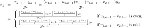
All the expressions within square brackets in the last equation are integers, since x₀ = b is odd. Note that updating the variables in the loop requires only the values of these variables available from the previous iteration. Therefore, we may drop the prefix k and call these variables x, y, u₁, u₂, v₁ and v₂. Moreover, the variables u₁ and u₂ need not be maintained and updated in every iteration, since the updating procedure for the other variables does not depend on the values of u₁ and u₂. We need the value of u₂ only at the end of the main loop, and this is available from the relation y = u₂b + v₂r maintained throughout the loop. The formula u₂b + v₂r = y = gcd(b, r) is then combined with the relations a = qb + r and gcd(a, b) = gcd(b, r) to get the final relation gcd(a, b) = v₂a + (u₂ – v₂q)b.

Algorithm 3.8 continues to work even when a < b, but in that case the initial reduction simply interchanges a and b and we forfeit the possibility of the reduction in size of the arguments (x and y) caused by the initial Euclidean division.

Finally, we remove the restriction that b is odd. We write a = 2^ra′ and b = 2^sb′ with a′, b′ odd and call Algorithm 3.8 with a′ and b′ as parameters (swapping a′ and b′, if a′ < b′) to compute integers d′, u′, v′ with d′ = gcd(a′, b′) = u′a′ + v′b′. Without loss of generality, assume that r ≥ s. Then d := gcd(a, b) = 2^sd′ = u′(2^sa′) + v′b. If r = s, then 2^sa′ = a and we are done. So assume that r > s. If u′ is even, we can extract a power of 2 from u′ and multiply 2^sa′ by this power. So let’s say that we have a situation of the form for some integers and , with odd, and for s ≤ t < r. We can rewrite this as . Since is even, this gives us , where τ > t and where is odd or τ = r. Proceeding in this way, we eventually reach a relation of the form d = u(2^ra′) + vb = ua + vb. It is easy to check that if (a′, b′) ≠ (1, 1), then the integers u and v obtained as above satisfy |u| < b and |v| < a.

3.3.4. Modular Arithmetic

So far, we have described how we can represent and work with the elements of . In cryptology, we are seemingly more interested in the arithmetic of the rings for multiple-precision integers n. We canonically represent the elements of by integers between 0 and n – 1.

Let a, . In order to compute a + b in , we compute the integer sum a + b, and, if a + b ≥ n, we subtract n from a + b. This gives us the desired canonical representative in . Similarly, for computing a – b in , we subtract b from a as integers, and, if the difference is negative, we add n to it. For computing , we multiply a and b as integers and then take the remainder of Euclidean division of this product by n.

Note that is invertible (that is, ) if and only if gcd(a, n) = 1. For , a ≠ 0, we call the extended (binary) gcd algorithm with a and n as the arguments and get integers d, u, v satisfying d = gcd(a, n) = ua+vn. If d > 1, a is not invertible modulo n. Otherwise, we have ua ≡ 1 (mod n), that is, a^–1 ≡ u (mod n). The extended gcd algorithm indeed returns a value of u satisfying |u| < n. Thus if u > 0, it is the canonical representative of a^–1, whereas if u < 0, then u + n is the canonical representative of a^–1.

Modular exponentiation

Another frequently needed operation in is modular exponentiation, that is, the computation of a^e for some and . Since a⁰ = 1 for all and since a^e = (a^–1)^–e for e < 0 and , we may assume, without loss of generality, that . Computing the integral power a^e followed by taking the remainder of Euclidean division by n is not an efficient way to compute a^e in . Instead, after every multiplication, we reduce the product modulo n. This keeps the size of the intermediate products small. Furthermore, it is also a bad idea to compute a^e as (· · ·((a·a)·a)· · ·a) which involves e – 1 multiplications. It is possible to compute a^e using O(lg e) multiplications and O(lg e) squarings in , as Algorithm 3.9 suggests. This algorithm requires the bits of the binary expansion of the exponent e, which are easily obtained by bit operations on the words of e.

The for loop iteratively computes b_i := a^{(e_r–1 ... e_i)₂} (mod n) starting from the initial value b_r := 1. Since (e_r–1 . . . e_i)₂ = 2(e_r–1 . . . e_i+1)₂ + e_i, we have (mod n). This establishes the correctness of the algorithm. The squaring (b²) and multiplication (ba) inside the for loop of the algorithm are computed in (that is, as integer multiplication followed by reduction modulo n). If we assume that e_r–1 = 1, then r = ⌈lg e⌉. The algorithm carries out r squares and ρ ≤ r multiplications in , where ρ is the number of bits of e, that are 1. On an average ρ = r/2. Algorithm 3.9 runs in time O((log e)(log n)²). Typically, e = O(n), so this running time is O((log n)³).

Algorithm 3.9. Modular exponentiation: square-and-multiply algorithm

Input: , . Output: . Steps: Let the binary expansion of e be e = (er–1 . . . e1e0)2, where each . b := 1. for (i = r – 1, . . . , 0) {    b := b2 (mod n).    /* Squaring */    if (ei = 1) b := ba (mod n).    /* Multiplication */ }

Now, we describe a simple variant of this square-and-multiply algorithm, in which we choose a small t and use the 2^t-ary representation of the exponent e. The case t = 1 corresponds to Algorithm 3.9. In practical situations, t = 4 is a good choice. As in Algorithm 3.9, multiplication and squaring are done in .

Algorithm 3.10. Modular exponentiation: windowed square-and-multiply algorithm

Input: , . Output: . Steps: Let e = (er–1 . . . e1e0)2t, where each . Compute and store  for l = 0, 1, . . . , 2t – 1.   /* Precomputation */ b := 1. for (i = r – 1, . . . , 0) {    for (j = 1, . . . , t) b := b2 (mod n).    /* Squaring */    b := baei (mod n).     /* Multiplication: Read aei from the precomputed table */ }

In Algorithm 3.10, the powers a^l, l = 0, 1, . . . , 2^t – 1, are precomputed using the formulas: a⁰ = 1, a¹ = a and a^l = a^l–1 · a for l ≥ 2. The number of squares inside the for loop remains (almost) the same as in Algorithm 3.9. However, the number of multiplications in this loop reduces at the expense of the precomputation step. For example, let n be an integer of bit length 1024 and let e ≈ n. A randomly chosen e of this size has about 512 one-bits. Therefore, the for loop of Algorithm 3.9 does about 512 multiplications, whereas with t = 4 Algorithm 3.10 does only 1024/4 = 256 multiplications with the precomputation step requiring 14 multiplications. Thus, the total number of multiplications reduces from (about) 512 to 14 + 256 = 270.

Montgomery exponentiation

During a modular exponentiation in , every reduction (computation of remainder) is done by the fixed modulus n. Montgomery exponentiation exploits this fact and speeds up each modular reduction at the cost of some preprocessing overhead.

Assume that the storage of n requires s ℜ-ary digits, that is, n = (n_s–1 . . . n₀)_ℜ (with n_s–1 ≠ 0). Take R := ℜ^s = 2^32s, so that R > n. As is typical in most cryptographic situations, n is an odd integer (for example, a big prime or a product of two big primes). Then gcd(ℜ, n) = gcd(R, n) = 1. Use the extended gcd algorithm to precompute n′ := –n^–1 (mod ℜ).

We associate with , where (mod n). Since R is invertible modulo n, this association gives a bijection of onto itself. This bijection respects the addition in : that is, in . Multiplication in , on the other hand, corresponds to , and can be implemented as Algorithm 3.11 suggests.

Algorithm 3.11. Montgomery multiplication

Input: and (Montgomery representations of x, ). Output: Montgomery representation of . Steps:

Montgomery multiplication works as follows. In the first step, it computes the integer product . The subsequent for loop computes (mod n). Since n′ ≡ –n^–1 (mod ℜ), the i-th iteration of the loop makes w_i = 0 (and leaves w_i–1, . . . ,w₀ unchanged). So when the for loop terminates, we have w₀ = w₁ = · · · = w_s–1 = 0: that is, is a multiple of ℜ^s = R. Therefore, is an integer. Furthermore, this is obtained by adding to a multiple of n: that is, for some integer k ≥ 0. Since R is coprime to n, it follows that (mod n). But this may be bigger than the canonical representative of . Since k is an integer with s ℜ-ary digits (so that k < R) and and n < R, it follows that . Therefore, if exceeds n – 1, a single subtraction suffices.

Computation of requires ≤ s² single-precision multiplications. One can use the optimized Algorithm 3.4 for that purpose. In case of squaring, and further optimizations (say, in the form of Karatsuba’s method) can be employed.

Each iteration of the for loop carries out s + 1 single-precision multiplications. (The reduction modulo ℜ is just returning the more significant word in the two-word product w_in′.) Since, the for loop is executed s times, Algorithm 3.11 performs a total of ≤ s² + s(s+1) = 2s² + s single-precision multiplications.

Integer multiplication (Algorithm 3.4) followed by classical modular reduction (Algorithm 3.6) does almost an equal number of single-precision multiplications, but also O(s) divisions of double-precision integers by single-precision ones. It turns out that the complicated for loop of Algorithm 3.6 is slower than the much simpler loop in Algorithm 3.11. But if precomputations in the Montgomery multiplication are taken into account, we do not tend to achieve a speed-up with this new technique. For modular exponentiations, however, precomputations need to be done only once: that is, outside the square-and-multiply loop, and Montgomery multiplication pays off. In Algorithm 3.12, we rewrite Algorithm 3.9 in terms of the Montgomery arithmetic. A similar rewriting applies to Algorithm 3.10.

Algorithm 3.12. Montgomery exponentiation

Input: , . Output: b = ae (mod n). Steps: /* Precomputations */ n′ := –n (mod ℜ). , . /* The square-and-multiply loop */ [View full size image]

Exercise Set 3.3

3.8	Let , ℜ > 1. Show that every can be represented uniquely as a tuple (as–1, . . . , a1, a0) for some (depending on a) with a = as–1ℜs–1 + · · · + a1ℜ + a0, 0 ≤ ai < ℜ for all i and as–1 ≠ 0. In this case, we write a as (as–1 . . . a0)ℜ or simply as as–1 . . . a0, when ℜ is understood from the context. ℜ is called the radix or base of this representation, as–1, . . . , a0 the (ℜ-ary) digits of a, as–1 the most significant digit, a0 the least significant digit and s the size of a with respect to the radix ℜ.
3.9	Let . Show that every can be written uniquely as a = asRs + as–1Rs–1 + · · · + a1R + a0 with each .
3.10	Negative radix Show that every integer can be written as a = as(–2)s + as–1(–2)s–1 + · · · + a1(–2) + a0 with . Moreover, if we force that as ≠ 0 for a ≠ 0 and that s = 0 for a = 0, argue that this representation is unique.
3.11	Investigate the relative merits and demerits of the following three representations (in C) of multiple-precision integers needed for cryptography. In each case, we have room for storing 256 ℜ-ary words, the actual size and a sign indicator. In the second and third representations, we use two extra locations (sizeIdx and signIdx) in the digit array for holding the size and sign information. /* Representation 1 */ typedef struct {    int size;    boolean sign;    ulong digits[256]; } cryptInt1; /* Representation 2 */ typedef ulong cryptInt2[258]; #define signIdx 0 #define sizeIdx 1 /* Representation 3 */ typedef ulong cryptInt3[258]; #define signIdx 256 #define sizeIdx 257 Remark: We recommend the third representation.
3.12	Write an algorithm that prints a multiple-precision integer in decimal and an algorithm that accepts a string of decimal digits (optionally preceded by a + or – sign) and stores the corresponding integer as a multiple-precision integer. Also write algorithms for input and output of multiple-precision integers in hexadecimal, octal and binary.
3.13	Write an algorithm which, given two multiple-precision integers a and b, compares the absolute values |a| and |b|. Also write an algorithm to compare a and b as signed integers.
3.14	Write an algorithm that uses the Euclidean gcd loop (Proposition 2.15) to compute the gcd d of two integers a and b. (Observe that gcd(a, b) = gcd(b, a rem b) for b ≠ 0.) Modify the Euclidean gcd algorithm of Part (a), so that for given integers a, b we obtain d, u, v with d = gcd(a, b) = ua + vb.
3.15	Describe a representation of rational numbers with exact multiple-precision numerators and denominators. Implement the arithmetic (addition, subtraction, multiplication and division) of rational numbers under this representation.
3.16	Sliding window exponentiation Suppose we want to compute the modular exponentiation ae (mod n). Consider the following variant of the square-and-multiply algorithm: Choose a small t (say, t = 4) and precompute a2t–1, a2t–1+1, . . . , a2t–1 modulo n. Do squaring for every bit of e, but skip the multiplication for zero bits in e. Whenever a 1 bit is found, consider the next t bits of e (including the 1 bit). Let these t bits represent the integer l, 2t–1 ≤ l ≤ 2t – 1. Multiply by al (mod n) (after computing usual t squares) and move right in e by t bit positions. Argue that this method works and write an algorithm based on this strategy. What are the advantages and disadvantages of this method over Algorithm 3.10?
3.17	Suppose we want to compute aebf (mod n), where both e and f are positive r-bit integers. One possibility is to compute ae and bf modulo n individually, followed by a modular multiplication. This strategy requires the running time of two exponentiations (neglecting the time for the final multiplication). In this exercise, we investigate a trick to reduce this running time to something close to 1.25 times the time for one exponentiation. Precompute ab (mod n). Inside the square-and-multiply loop, either skip the multiplication or multiply by a, b or ab, depending upon the next bits in the two exponents e and f. Complete the details of this algorithm. Deduce that, on an average, the running time of this algorithm is as declared above.
3.18	Let , m ≠ 1. An addition chain for m of length l is a sequence 1 = a1, a2, . . . , al = m of natural numbers such that for every index i, 2 ≤ i ≤ l, there exist indices i1, i2 < i with ai = ai1 + ai2. (It is allowed to have i1 = i2.) If 1 = a1, a2, . . . , al = m is an addition chain for m and if j1, j2, . . . , jl is a permutation of 1, 2, . . . , l with aj1 ≤ aj2 ≤ · · · ≤ ajl, show that aj1, aj2, . . . , ajl is also an addition chain for m. It, therefore, suffices to consider sorted addition chains only. Show that m has an addition chain of length ≤ 2 ⌈lg m⌉. [H] Let G be a (multiplicative) group and . Design an algorithm for computing gm given an addition chain for m. What is the complexity of the algorithm (in terms of the length of the given addition chain)? Show that Algorithms 3.9 and 3.10 use addition chains for e of lengths ≤ 2 ⌈lg e⌉.