
3.4. Elementary Number-theoretic Computations
Now that we know how to work in ![]() and in the residue class rings
and in the residue class rings ![]() ,
, ![]() , we address some important computational problems associated with these rings. In this chapter, we restrict ourselves only to those problems that are needed for setting up various cryptographic protocols.
, we address some important computational problems associated with these rings. In this chapter, we restrict ourselves only to those problems that are needed for setting up various cryptographic protocols.
3.4.1. Primality Testing
One of the simplest and oldest questions in algorithmic number theory is to decide if a given integer ![]() , n > 1, is prime or composite. Practical primality testing algorithms are based on randomization techniques. In this section, we describe the Monte Carlo algorithm due to Miller and Rabin. The obvious question that comes next is to find one (or all) of the prime factors of an integer, deterministically or probabilistically proven to be composite. This is the celebrated integer factorization problem and will be formally introduced in Section 4.2. In spite of the apparent proximity between the primality testing and the integer factoring problems, they currently have widely different (known) complexities. Primality testing is easy and thereby promotes efficient setting up of cryptographic protocols. On the other hand, the difficulty of factoring integers protects these protocols against cryptanalytic attacks.
, n > 1, is prime or composite. Practical primality testing algorithms are based on randomization techniques. In this section, we describe the Monte Carlo algorithm due to Miller and Rabin. The obvious question that comes next is to find one (or all) of the prime factors of an integer, deterministically or probabilistically proven to be composite. This is the celebrated integer factorization problem and will be formally introduced in Section 4.2. In spite of the apparent proximity between the primality testing and the integer factoring problems, they currently have widely different (known) complexities. Primality testing is easy and thereby promotes efficient setting up of cryptographic protocols. On the other hand, the difficulty of factoring integers protects these protocols against cryptanalytic attacks.
Definition 3.2.
|
Let n be an odd integer greater than 1 and let |
By Fermat’s little theorem, a prime p is a pseudoprime to every base ![]() with gcd(a, p) = 1. However, the converse of this is not true. By Exercise 3.19, n is not a pseudoprime to at least half of the bases in
with gcd(a, p) = 1. However, the converse of this is not true. By Exercise 3.19, n is not a pseudoprime to at least half of the bases in ![]() , provided that there is at least one such base in
, provided that there is at least one such base in ![]() . Unfortunately, there exist composite integers m, known as Carmichael numbers, such that m is a pseudoprime to every base
. Unfortunately, there exist composite integers m, known as Carmichael numbers, such that m is a pseudoprime to every base ![]() . The smallest Carmichael number is 561 = 3 × 11 × 17. Exercises 3.21 and 3.22 investigate some properties of these numbers. Though Carmichael numbers are not very abundant in nature (
. The smallest Carmichael number is 561 = 3 × 11 × 17. Exercises 3.21 and 3.22 investigate some properties of these numbers. Though Carmichael numbers are not very abundant in nature (![]() ), they are still infinite in number. So a robust primality test requires n to satisfy certain constraints in addition to being a pseudoprime to one or more bases. The following constraint is due to Solovay and Strassen.
), they are still infinite in number. So a robust primality test requires n to satisfy certain constraints in addition to being a pseudoprime to one or more bases. The following constraint is due to Solovay and Strassen.
Definition 3.3.
|
Let n be an odd integer > 1 and let |
By Euler’s criterion (Proposition 2.21), if p is a prime and gcd(a, p) = 1, then p is an Euler pseudoprime to the base a. The converse in not true, in general, but if n is composite, then n is an Euler pseudoprime to at most φ(n)/2 bases in ![]() (Exercise 3.20). This, in turn, implies that if n is an Euler pseudoprime to t randomly chosen bases in
(Exercise 3.20). This, in turn, implies that if n is an Euler pseudoprime to t randomly chosen bases in ![]() , then the chance that n is composite is no more than 1/2t. This observation leads to a Monte Carlo algorithm for testing the primality of an integer, where the probability of error (1/2t) can be made arbitrarily small by choosing large values of t. A more efficient algorithm can be developed using the following concept due to Miller and Rabin.
, then the chance that n is composite is no more than 1/2t. This observation leads to a Monte Carlo algorithm for testing the primality of an integer, where the probability of error (1/2t) can be made arbitrarily small by choosing large values of t. A more efficient algorithm can be developed using the following concept due to Miller and Rabin.
Definition 3.4.
|
Let n be an odd integer > 1 with n – 1 = 2rn′, r := v2(n – 1) > 0, n′ odd, and let |
The rationale behind this definition is the following. If for some ![]() we have an–1 ≢ 1 (mod n), we conclude with certainty that n is composite. So assume that an–1 ≡ 1 (mod n) and consider the powers bi := a2in′ (mod n) for i = 0, 1, . . . , r to see how the sequence b0, b1, . . . eventually reaches br ≡ 1 (mod n). If b0 ≡ 1 (mod n) already, this dynamics is clear. If, on the other hand, we have an i such that bi ≢ 1 (mod n), whereas bi+1 ≡ 1 (mod n), then bi is a square root of 1 modulo n. If n is a prime, the only square roots of 1 modulo n are ±1 and so n must be a strong pseudoprime to the base a. On the other hand, if n is composite but not the power of a prime, then 1 has at least two non-trivial square roots (that is, square roots other than ±1) modulo n (Exercise 3.30). We hope to find one such non-trivial square root of 1 in the sequence b0, b1, . . . , br–1 and if we are successful, the compositeness of n is proved with certainty.
we have an–1 ≢ 1 (mod n), we conclude with certainty that n is composite. So assume that an–1 ≡ 1 (mod n) and consider the powers bi := a2in′ (mod n) for i = 0, 1, . . . , r to see how the sequence b0, b1, . . . eventually reaches br ≡ 1 (mod n). If b0 ≡ 1 (mod n) already, this dynamics is clear. If, on the other hand, we have an i such that bi ≢ 1 (mod n), whereas bi+1 ≡ 1 (mod n), then bi is a square root of 1 modulo n. If n is a prime, the only square roots of 1 modulo n are ±1 and so n must be a strong pseudoprime to the base a. On the other hand, if n is composite but not the power of a prime, then 1 has at least two non-trivial square roots (that is, square roots other than ±1) modulo n (Exercise 3.30). We hope to find one such non-trivial square root of 1 in the sequence b0, b1, . . . , br–1 and if we are successful, the compositeness of n is proved with certainty.
A complete residue system modulo an odd composite n contains at most n/4 bases to which n is a strong pseudoprime. The proof of this fact is somewhat involved (though elementary) and can be found elsewhere, for example, in Chapter V of Koblitz [153]. Here, we concentrate on the Monte Carlo Algorithm 3.13 known as the Miller–Rabin primality test and based on this observation.
Algorithm 3.13. Miller–Rabin primality test
Whenever Algorithm 3.13 outputs n is composite, it is correct. On the other hand, if it certifies n as prime, there is a probability δ that n is composite. This probability can be made very small by choosing a suitably large value of the iteration count t. For cryptographic applications, δ ≤ 1/280 is considered sufficiently safe. In view of the first statement of the last paragraph, we can take t = 40 to meet this error bound. In practice, much smaller values of t offer the desired confidence. For example, if n is of bit length 250, 500, 750 or 1000, the respective values t = 12, 6, 4 and 3 suffice.
Although, in Algorithm 3.13, we have chosen a to be an arbitrary integer between 2 and n – 2, there is apparently no harm, if we choose a randomly in the interval 2 ≤ a < 232. In fact, such a choice of single-precision bases is desirable, because that makes the exponentiation an′ (mod n) more efficient (See Algorithm 3.9). A typical cryptographic application loads at start-up a precalculated table of small primes (say, the first thousand primes). Choosing the bases randomly from this list of small primes is indeed a good idea.
Deterministic primality proving
While the Miller–Rabin algorithm settles the primality testing problem in a practical sense, it is, after all, a randomized algorithm. It is interesting, at the minimum theoretically, to investigate the deterministic complexity of primality testing. There has been a good amount of research in this line. Let us sketch here the history of deterministic primality proving, without going to rigorous mathematical details.
One natural strategy to check for the primality of a positive integer n is to factor it. However, factoring integers is a computationally difficult problem. Primality proving has been found to be a much easier computational exercise. That is, one need not factorize n explicitly in order to claim about the primality of n.
The (seemingly) first modern primality testing algorithm is due to Miller[204]. This algorithm is deterministic polynomial-time, provided that the extended Riemann hypothesis or ERH (Conjecture 2.3) is true. Since the ERH is still an unsolved problem in mathematics, it cannot be claimed with certainty if Miller’s test is really a polynomial-time algorithm. Rabin [248] provided a version of Miller’s test which is unconditionally polynomial-time, but is, at the same time, randomized. This is what we have discussed earlier under the name Miller–Rabin primality test. This is a Monte Carlo algorithm which produces the answer no (composite) with certainty, but the answer yes (prime) with some (small) probability of error. Solovay and Strassen’s test [287] based on Definition 3.3 is another no-biased randomized polynomial-time primality test and can be made deterministically polynomial-time under the ERH.
Adleman and Huang [3], using the work of Goldwasser and Kilian [116], provide a yes-biased randomized primality-proving algorithm that runs in expected polynomial time unconditionally. Adleman et al. [4] propose the first deterministic algorithm that runs unconditionally in time less than fully exponential (in log n). Its (worst) running time is (ln n)O(ln ln ln n), which is still not polynomial. (The exponent ln ln ln n grows very slowly with n, but still is not a constant.)
In August 2002, Agarwal, Kayal and Saxena came up with the first deterministic primality testing algorithm that runs in polynomial time unconditionally, that is, under no unproven assumptions. This algorithm, popularly abbreviated as the AKS algorithm, is based on the observation that n is prime if and only if (X + a)n ≡ Xn + a (mod n) for every ![]() (Exercise 3.26). A naive application of this observation requires computing an exponential number of coefficients in the binomial expansion of (X + a)n. The AKS algorithm gets around with this difficulty by checking the new congruence
(Exercise 3.26). A naive application of this observation requires computing an exponential number of coefficients in the binomial expansion of (X + a)n. The AKS algorithm gets around with this difficulty by checking the new congruence
Equation 3.2
![]()
for some polynomial h(X) of small degree. Here the notation (mod n, h(X)) means modulo the ideal ![]() of
of ![]() . If deg h(X) is bounded by a polynomial in log n, (X + a)n (and also Xn + a) can be computed modulo n, h(X) in polynomial time. However, reduction modulo h(X) may allow a composite n to satisfy the new congruence. Agarwal et al. took h(X) := Xr –1 for some prime r = O(ln6 n) with r – 1 having a prime divisor
. If deg h(X) is bounded by a polynomial in log n, (X + a)n (and also Xn + a) can be computed modulo n, h(X) in polynomial time. However, reduction modulo h(X) may allow a composite n to satisfy the new congruence. Agarwal et al. took h(X) := Xr –1 for some prime r = O(ln6 n) with r – 1 having a prime divisor ![]() ln n. From a result in analytic number theory due to Fouvry, such a prime r always exists. Congruence (3.2) is verified for this h(X) and for at most
ln n. From a result in analytic number theory due to Fouvry, such a prime r always exists. Congruence (3.2) is verified for this h(X) and for at most ![]() ln n values of a. An elementary proof presented in Agarwal et al. [5] demonstrates that this suffices to conclude deterministically and unconditionally about the primality of n. The AKS algorithm in this form runs in time O~(ln12 n).
ln n values of a. An elementary proof presented in Agarwal et al. [5] demonstrates that this suffices to conclude deterministically and unconditionally about the primality of n. The AKS algorithm in this form runs in time O~(ln12 n).
Lenstra and Pomerance [175] have reduced the running time of the AKS algorithm to O~(ln6 n). The AKS paper comes with another conjecture which, if true, yields a O~(ln3 n) deterministic primality-proving algorithm.
Conjecture 3.1. AKS conjecture
|
Let n be an odd integer > 1, and (X – 1)n ≡ Xn – 1 (mod n, Xr – 1), then either n is prime or n2 ≡ 1 (mod r). |
It remains an open question whether a future version of the AKS algorithm would supersede the Miller–Rabin test in terms of performance. As long as the answers are not favourable to the AKS algorithm, these new theoretical endeavours do not seem to have sufficient impacts on cryptography. Primes certified by the Miller–Rabin test are at present secure enough for all applications. Nonetheless, the AKS breakthrough has solid theoretical implications and deserves mention in a prime context.
3.4.2. Generating Random Primes
If a random prime of a given bit length t is called for, we can keep on generating random odd integers of bit length t and check these integers for primality using the Miller–Rabin test. The prime number Theorem 2.20 ascertains that after O(t) iterations we expect to find a prime. A somewhat similar but reasonably faster algorithm is discussed in Exercise 4.14. We will henceforth call random primes of a given bit length and having no additional imposed properties as naive primes. Naive primes are often not cryptographically secure, because the primes used in many protocols should satisfy certain properties in order to preclude some known cryptanalytic attacks.
Definition 3.5.
|
Let p be an odd prime. Then p is called a safe prime, if (p – 1)/2 is also a prime, whereas p is called a strong prime, if
In cryptography, a large prime divisor typically refers to one with bit length ≥ 160. |
A random safe prime of a given bit length t can be found by generating a random sequence of natural numbers n congruent to 3 modulo 4 and of bit length t, until one is found for which both n and (n – 1)/2 are primes (as certified by the Miller–Rabin primality test). The prime number theorem once again implies that this search is expected to terminate after O(t2) iterations.
For generating a random strong prime p of bit length t, we first generate q′ and q″ and then q and finally p. (See the notations of Definition 3.5.) Algorithm 3.14 describes Gordon’s algorithm in which the bit lengths l and l′ of q and q′ are nearly t/2 and the bit length l″ of q″ is slightly smaller than l′. In our concrete implementation of the algorithm, we choose l := ⌈t/2⌉ – 2, l′ := ⌊t/2⌋ – 20 and l″ := ⌈t/2⌉ – 22. If t is sufficiently large (say, t ≥ 400), the prime divisors q, q′ and q″ are then cryptographically large.
The simple check that Gordon’s algorithm correctly computes a strong prime of bit length t with q, q′ and q″ as in Definition 3.5 is based on Fermat’s little theorem and is left to the reader. Note that with our choice of l, l′ and l″, the loop variables i and j run through single-precision values only, thereby making arithmetic involving them efficient. Also note that the ranges over which i and j vary are sufficiently large so that we expect the (outer) while loop to be executed only once. This implementation has a tendency to generate smaller values of q and p (with the given bit sizes). In practice, this is not a serious problem and can be avoided, if desired, by choosing random values of i and j from the indicated ranges.
Algorithm 3.14. Gordon’s strong-prime generator
|
Output: A strong prime p of bit length t. Steps: l := ⌈t/2⌉ – 2, l′ := ⌊t/2⌋ – 20, l″ := ⌈t/2⌉ – 22. while (1) { |
Gordon’s algorithm takes only nominally more expected running time than that needed by the algorithm discussed at the beginning of Section 3.4.2 for generating naive primes of the same bit length. On the other hand, safe primes are much costlier to generate and may be avoided, unless the situation specifically demands their usage.
3.4.3. Modular Square Roots
Determination of square roots modulo a prime p is frequently needed in cryptographic applications. In this section, we assume that p is an odd prime and want to compute the square roots of ![]() , gcd(a, p) = 1, modulo p, provided that a is a quadratic residue modulo p, that is, if
, gcd(a, p) = 1, modulo p, provided that a is a quadratic residue modulo p, that is, if ![]() . Using the Jacobi symbol the value
. Using the Jacobi symbol the value ![]() can be computed efficiently as Algorithm 3.15 suggests.
can be computed efficiently as Algorithm 3.15 suggests.
The correctness of Algorithm 3.15 follows from the properties of the Jacobi symbol (Proposition 2.22 and Theorem 2.19). The value of (–1)(b2–1)/8 is determined by the value of b modulo 8, that is, by the three least significant bits of b:
![]()
Similarly, (–1)(a – 1)(b – 1)/4 can be computed using only the second least significant bits of a and b as:
![]()
If ![]() , our next task is to compute
, our next task is to compute ![]() with x2 ≡ a (mod p). If one such x is found, the other square root of a modulo p is –x ≡ p – x (mod p). If p ≡ 3 (mod 4) or p ≡ 5 (mod 8), we have explicit formulas for a square root x. The remaining case, namely p ≡ 1 (mod 8), is somewhat complicated. In this case, we use the probabilistic algorithm due to Tonelli and Shanks. The details are given in Algorithm 3.16. The explicit formulas for the first two cases are easy to verify. We now prove the correctness of the algorithm in the remaining case.
with x2 ≡ a (mod p). If one such x is found, the other square root of a modulo p is –x ≡ p – x (mod p). If p ≡ 3 (mod 4) or p ≡ 5 (mod 8), we have explicit formulas for a square root x. The remaining case, namely p ≡ 1 (mod 8), is somewhat complicated. In this case, we use the probabilistic algorithm due to Tonelli and Shanks. The details are given in Algorithm 3.16. The explicit formulas for the first two cases are easy to verify. We now prove the correctness of the algorithm in the remaining case.
Algorithm 3.15. Computation of the Legendre symbol
|
Input: An odd prime p and an integer a, 1 ≤ a < p. Output: The Legendre symbol Steps:
/* The Euclidean loop */ 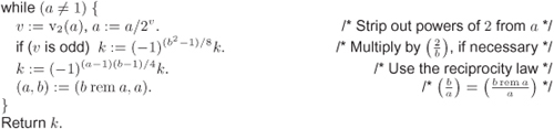
|
Since ![]() is cyclic and has order p – 1 = 2vq, the 2-Sylow subgroup G of
is cyclic and has order p – 1 = 2vq, the 2-Sylow subgroup G of ![]() has order 2v and is also cyclic. Let g be a generator of G. By Euler’s criterion, aq is a square in G and, therefore, aqge = 1 (in G) for some even integer e, 0 ≤ e < 2v, and x ≡ a(q + 1)/2ge/2 (mod p) is a square root of a modulo p.
has order 2v and is also cyclic. Let g be a generator of G. By Euler’s criterion, aq is a square in G and, therefore, aqge = 1 (in G) for some even integer e, 0 ≤ e < 2v, and x ≡ a(q + 1)/2ge/2 (mod p) is a square root of a modulo p.
A generator g of G can be obtained by choosing random elements b from ![]() and computing the Legendre symbol
and computing the Legendre symbol ![]() . It is easy to see that
. It is easy to see that ![]() . Furthermore, bq is a generator of G if and only if
. Furthermore, bq is a generator of G if and only if ![]() . Finding a quadratic non-residue in
. Finding a quadratic non-residue in ![]() is the probabilistic part of the algorithm. Since exactly half of the elements of
is the probabilistic part of the algorithm. Since exactly half of the elements of ![]() are quadratic non-residues, one expects to find one after a few random trials. In order to make the exponentiation bq efficient, b should be chosen as single-precision integers. The while loop of the algorithm computes the multiplier ge/2 in x using O(v) iterations by successively locating the 1 bits of e starting from the least significant end.
are quadratic non-residues, one expects to find one after a few random trials. In order to make the exponentiation bq efficient, b should be chosen as single-precision integers. The while loop of the algorithm computes the multiplier ge/2 in x using O(v) iterations by successively locating the 1 bits of e starting from the least significant end.
To sum up, square roots modulo a prime can be computed in probabilistic polynomial time. Computing square roots modulo a composite integer n is, on the other hand, a very difficult problem, unless the complete factorization of n is known (see Section 4.2 and Exercise 3.29).
Exercise Set 3.4
| 3.19 | Let Algorithm 3.16. Modular square root | |
| 3.20 | Let
| |
| 3.21 | Let
| |
| 3.22 |
| |
| 3.23 | Fermat’s test for prime numbers Let | |
| 3.24 | Pépin’s test for Fermat numbers Show that the Fermat number n := 22k + 1 is prime if and only if 3(n – 1)/2 ≡ –1 (mod n). | |
| 3.25 | Write an algorithm that, given natural numbers t, l with l < t, outputs a (probable) prime p of bit length t such that p – 1 has a (probable) prime divisor q of bit length l. | |
| 3.26 | Let
| |
| 3.27 | Modify Algorithm 3.15 to compute the (generalized) Jacobi symbol | |
| 3.28 | A Implement the Chinese remainder theorem for integers, that is, write an algorithm that takes as input pairwise relatively prime moduli | |
| 3.29 | Let f(X) be a non-constant polynomial in
| |
| 3.30 | Let | |
| 3.31 | Show that Algorithm 3.17 correctly computes Algorithm 3.17. Integer square root
| |
| 3.32 |
|