
Network Analysis
MA Laughton, BASc, PhD, DSc(Eng), FREng, FIEE, Formerly of Queen Mary & Westfield College. University of London (Sections 3.3.1–3.3.5)
3.1 Introduction
In an electrical network, electrical energy is conveyed from sources to an array of interconnected branches in which energy is converted, dissipated or stored. Each branch has a characteristic voltage–current relation that defines its parameters. The analysis of networks is concerned with the solution of source and branch currents and voltages in a given network configuration. Basic and general network concepts are discussed in Section 3.2. Section 3.3 is concerned with the special techniques applied in the analysis of power-system networks.
3.2 Basic network analysis
Given the sources (generators, batteries, thermocouples, etc.), the network configuration and its branch parameters, then the network solution proceeds through network equations set up in accordance with the Kirchhoff laws.
3.2.1.1 Sources
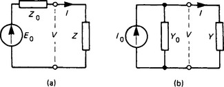
In most cases a source can be represented as in Figure 3.1(a) by an electromotive force (e.m.f.) E0 acting through an internal series impedance Z0 and supplying an external ‘load’ Z with a current I at a terminal voltage V. This is the Helmholtz–Thevenin equivalent voltage generator. As regards the load voltage V and current I, the source could equally well be represented by the Helmholtz–Norton equivalent current generator in Figure 3.1(b), comprising a source current I0 shunted by an internal admittance Y0 which is effectively in parallel with the load of admittance Y. Comparing the two forms for the same load current I and terminal voltage V in a load of impedance Z or admittance Y = 1/Z, we have:
| Voltage generator | Current generator |
| V = E0 − IZ0 | I = I0 − VY0 |
| I = (E0 − V)/Z0 | V = (I0 − I) / Y0 |
| = E0/Z0 − V/Z0 | = I0/Y0 − I / Y0 |
| = I0 − V Y0 | = E0 − IZ0 |
These are identical provided that I0 = E0/Z0 and Y0 = 1/Z0. The identity applies only to the load terminals, for internally the sources have quite different operating conditions. The two forms are duals. Sources with Z0 = 0 and Y0 = 0 (so that V = E0 and I = I0) are termed ideal generators.
3.2.1.2 Parameters
When a real physical network is set up by interconnecting sources and loads by conducting wires and cables, all parts (including the connections) have associated electric and magnetic fields. A resistor, for example, has resistance as the prime property, but the passage of a current implies a magnetic field, while the potential difference (p.d.) across the resistor implies an electric field, both fields being present in and around the resistor. In the equivalent circuit drawn to represent the physical one it is usual to lump together the significant resistances into a limited number of lumped resistances. Similarly, electric-field effects are represented by lumped capacitance and magnetic-field effects by lumped inductance. The equivalent circuit then behaves like the physical prototype if it is so constructed as to include all significant effects.
The lumped parameters can now be considered to be free from ‘residuals’ and pure in the sense that simple laws of behaviour apply. These are indicated in Figure 3.2.
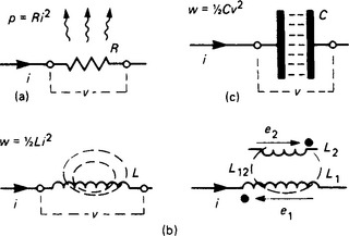
(a) Resistance For a pure resistance R carrying an instantaneous current i, the p.d. is v = Ri and the rate of heat production is p = vi = Ri2. Alternatively, if the conductance G = 1/R is used, then i = Gv and p = vi = Gv2. There is a constant relation
(b) Inductance With a self-inductance L, the magnetic linkage is Li, and the source voltage is required only when the linkage changes, i.e. v = d(Li)/dt = L(di/dt). An inductor stores in its magnetic field the energy w = ½Li2. The behaviour equations are
Two inductances L1 and L2 with a common magnetic field have a mutual inductance L12 = L21 such that an e.m.f. is induced in one when current changes in the other:
The direction of the e.m.f.s depends on the change (increase or decrease) of current and on the ‘sense’ in which the inductors are wound. The ‘dot convention’ for establishing the sense is to place a dot at one end of the symbol for L1, and a dot at that end of L2 which has the same polarity as the dotted end of L1 for a given change in the common flux.
(c) Capacitance The stored charge q is proportional to the p.d. such that q = Cv. When v is changed, a charge must enter or leave at the rate i = dq/dt = C(dv/dt). The electric-field energy in a charged capacitor is w = ½Cv2. Thus
It can be seen that there is a duality between the inductor and the capacitor. Some typical cases of the behaviour of pure parameters are given in Figures 2.3, 2.21 and 2.28.
A more concise representation of the behaviour of pure parameters uses the differential operator p for d/dt and the inverse 1/p for the integral operator: then
For the steady-state direct-current (d.c.) case, p = 0. For steady-state sinusoidal alternating current (a.c), p = jω, giving for L and C the forms j ωL and 1/j ωC where ω is the angular frequency. In general, L p and 1/C p are the operational impedance parameters.
3.2.1.3 Configuration
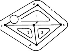
The assembly of sources and loads forms a network of branches that interconnect nodes (junctions) and form meshes. The seven-branch network shown in Figure 3.3 has five nodes (a, b, c, d, e) and four meshes (1, 2, 3, 4). Branch ab contains a voltage source; the other branches have (unspecified) impedance parameters. Inspection shows that not all the meshes are independent: mesh 4, for example, contains branches already accounted for by meshes 1, 2 and 3. Further, if one node (say, e) is taken as a reference node, the voltages of nodes a, b, c and d can be taken as their p.d.s with respect to node e. The network is then taken as having b = 7 branches, m = 3 independent meshes and n = 4 independent nodes. In general, m = b − n.
3.2.2 Network laws
The behaviour of networks (i.e. the branch currents and node voltages for given source conditions) is based on the two Kirchhoff laws (Figure 3.4).
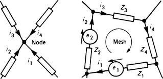
(1) Node law The total current flowing into a node is zero, Σi = 0. The sum of the branch currents flowing into a node must equal the sum of the currents flowing from it; this is a result of the ‘particle’ nature of conduction current.
(2) Mesh law The sum of the voltages around a closed mesh is zero, Σv = 0. A rise of potential in sources is absorbed by a fall in potential in the successive branches forming the mesh. This is the result of the nature of a network as an energy system.
The Kirchhoff laws apply to all networks. Whether the evaluation of node voltages and mesh currents is tractable or not depends not only on the complexity of the network configuration but also on the branch parameters. These may be active or passive (i.e. containing or not containing sources), linear or non-linear. Non-linearity, in which the parameters are not constant but depend on the voltage and/or current magnitude and polarity, is in fact the normal condition, but where possible the minor non-linearities are ignored in order to permit the use of greatly simplified analysis and the principle of superposition.
3.2.2.1 Superposition
In a strictly linear network, the current in any branch is the sum of the currents due to each source acting separately, all other sources being replaced meantime by their internal impedances. The principle applies to voltages and currents, but not to powers, which are current–voltage products.
3.2.3 Network solution
A general solution presents the voltages and currents everywhere in the network; it is initiated by the solution simultaneously of the network equations in terms of voltages, currents and parameters.
The Kirchhoff laws can be applied systematically by use of the Maxwell circulating-current process. To each mesh is assigned a circulating current, and the laws are applied with due regard to the fact that certain branches, being common to two adjacent meshes, have net currents given by the superposition of the individual mesh currents postulated. Generalising, the network can be considered as either (i) a set of independent nodes with appropriate node-voltage equations, or (ii) a set of independent meshes with corresponding mesh-current equations.
3.2.3.1 Mesh-current equations
This is a formulation of the Maxwell circulating-current process. If source e.m.f.s are written as E, currents as I and impedances as Z, then for the m independent meshes
Here Z11, Z22, …., Zmm are the self-impedances of meshes 1, 2, …, m, i.e. the total series impedance around each of the chosen meshes; and Z12, Zpq, …, are the mutual impedances of meshes 1 and 2, p and q, …, i.e. the impedances common to the designated meshes.
The mutual impedance is defined as follows. Zpq is the p.d. per ampere of Iq in the direction of Ip, and Zqp is the p.d. per ampere of Ip in the direction of Iq. The sign of a mutual impedance depends on the current directions chosen for the meshes concerned. If the network is co-planar (i.e. it can be drawn on a diagram with no cross-over) it is usual to select a single consistent direction—say clockwise—for each mesh current. In such a case the mutual impedances are negative because the currents are oppositely directed in the common branches.
3.2.3.2 Node-voltage equations
Of the network nodes, one is chosen as a reference node to which all other node voltages are related. The sources are represented by current generators feeding specified currents into their respective nodes and the branches are in terms of admittance Y. Then for the n independent nodes
Here Yaa, Ybb, …, Ynn are the self-admittances of nodes a, b, …, n, i.e. the sum of the admittances terminating on nodes a, b, …, n; and Yab, Ypq, …, are the mutual admittances, those that link nodes a and b, p and q, …, respectively, and which are usually negative.
The mesh-current and node-voltage methods are general and basic; they are applicable to all network conditions. Simplified and auxiliary techniques are applied in special cases.
3.2.3.3 Techniques
Steady-state conditions: Transient phenomena are absent. For d.c. networks the constant current implies absence of inductive effects, and capacitors (having a constant charge) are equivalent to an open circuit. Only resistance is taken into account, using the Ohm law.
For a.c. networks with sinusoidal current and voltage, complexor algebra, phasor diagrams, locus diagrams and symmetrical components are used, while for a.c. networks with periodic but non-sinusoidal waveforms harmonic analysis with superposition of harmonic components is employed.
3.2.4 Network theorems
Network theorems can simplify complicated networks, facilitate the solution of specific network branches and deal with particular network configurations (such as two-ports). They are applicable to linear networks for which superposition is valid, and to any form (scalar, complexor, or operational) of voltage, current, impedance and admittance. In the following, the Ohm and Kirchhoff laws, and the reciprocity and compensation theorems, are basic; star–delta transformation and the Millman theorem are applied to network simplification; and the Helmholtz–Thevenin and Helmholtz–Norton theorems deal with specified branches of a network. Two-ports are dealt with in Section 3.2.5.
3.2.4.1 Ohm (Figure 3.2(a))
For a branch of resistance R or conductance G,
Summation of resistances R1, R2, …, in series or parallel gives
The Ohm law is generalised for a.c. and transient cases by I = V/Z or I(p)= V(p)/Z(p), where p is the operator d/dt.
3.2.4.3 Reciprocity
If an e.m.f. in branch P of a network produces a current in branch Q, then the same e.m.f. in Q produces the same current in P. The ratio of the e.m.f. to the current is then the transfer impedance or admittance.
3.2.4.4 Compensation
For given circuit conditions, any impedance Z in a network that carries a current I can be replaced by a generator of zero internal impedance and of e.m.f. E = −IZ. Further, if Z is changed by ΔZ, then the effect on all other branches is that which would be produced by an e.m.f. −IΔ Z in series with the changed branch. By use of this theorem, if the network currents have been solved for given conditions, the effect of a changed branch impedance can be found without re-solving the entire network.
3.2.4.5 Star—delta (Figure 3.5)
At a given frequency (including zero) a three-branch star impedance network can be replaced by a three-branch delta network, and conversely. For a star Za, Zb, Zc to be equivalent between terminals AB, BC, CA to a delta Z1, Z2, Z3, it is necessary that
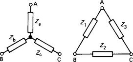
where Z = Z1+ Z2 + Z3. The general star–mesh conversion concerns the replacement of an n-branch star by a mesh of ½n(n − 1) branches, but not conversely; and as the number of mesh branches is greater than the number of star branches when n > 3, the conversion is only rarely of use.
3.2.4.6 Millman (Figure 3.6)
The Millman theorem is also known as the parallel-generator theorem. The common terminal voltage of a number of sources connected in parallel to a common load of impedance Z is V = IscZp, where Ix is the sum of the short-circuit currents of the individual source branches and Zp is the effective impedance of all the branches in parallel, including the load Z. If E1 and E2 are the e.m.f.s of two sources with internal impedances Z1 and Z2 connected in parallel to supply a load Z, and if I1, and I2 are the currents contributed by these sources to the load Z, then their common terminal voltage V must be
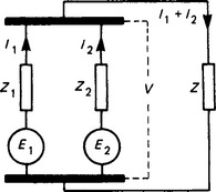
The term in parentheses on the left-hand side of the equation is the effective admittance of all the branches in parallel. The right-hand side of the equation is the sum of the individual source short-circuit currents, totalling Isc. Thus V = IscZP. The theorem holds for any number of sources.
3.2.4.7 Helmholtz–Thevenin (Figure 3.7)
The current in any branch Z of a network is the same as if that branch were connected to a voltage source of e.m.f. E0 and internal impedance Z0, where E0 is the p.d. appearing across the branch terminals when they are open-circuited and Z0 is the impedance of the network looking into the branch terminals with all sources represented by their internal impedance.
In Figure 3.7, the network has a branch AB in which it is required to find the current. The branch impedance Z is removed, and a p.d. E0 appears across AB. With all sources replaced by their internal impedance, the network presents the impedance Z0 to AB. The current in Z when it is replaced into the original network is
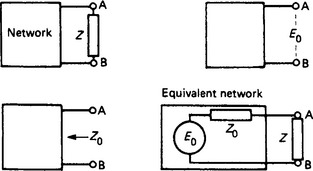
The whole network apart from the branch AB has been replaced by an equivalent voltage source, resulting in the simplified condition of Figure 3.1(a).
3.2.4.8 Helmholtz–Norton
The Helmholtz–Norton theorem is the dual of the Helmholtz–Thevenin theorem. The voltage across any branch Y of a network is the same as if that branch were connected to a current source I0 with internal shunt admittance Y0, where I0 is the current between the branch terminals when short circuited and Y0 is the admittance of the network looking into the branch terminals with all sources represented by their internal admittance. Then across the terminals AB in Figure 3.7 the voltage is
Thus the whole network apart from the branch AB has been replaced by an equivalent current source, i.e. the system in Figure 3.1(b).
3.2.5 Two-ports
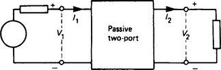
In power and signal transmission, input voltage and current at one port (i.e. one terminal-pair) yield voltage and current at another port of the interconnecting network. Thus in Figure 3.8a voltage source at the input port 1 delivers to the passive network a voltage V1 and a current I1. The corresponding values at the output port 2 are V2 and I2.
3.2.5.1 Lacour
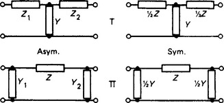
According to the theorem originated by Lacour, any passive linear network between two ports can be replaced by a two-mesh or T network, and in general no simpler form can be found. Such a result is obtained by iterative star–delta conversion to give the T equivalent; by one more star–delta conversion the π-equivalent is obtained (Figure 3.9). In general, the equivalent networks are asymmetric; in some cases, however, they are symmetric. It can be shown that a passive two-port has the input and output voltages and currents related by
where ABCD are the general two-port parameters, constants for a given frequency and with AD − BC = 1. The conventions for voltage polarity and current direction are those given in Figure 3.8.
3.2.5.2 T network
Consider the asymmetric T in Figure 3.9. Application of the Kirchhoff laws gives
Hence in terms of the series and parallel branch components
Multiplication shows that AD − BC = 1.
3.2.5.3 π network
In a similar way, the general parameters for the asymmetric case are
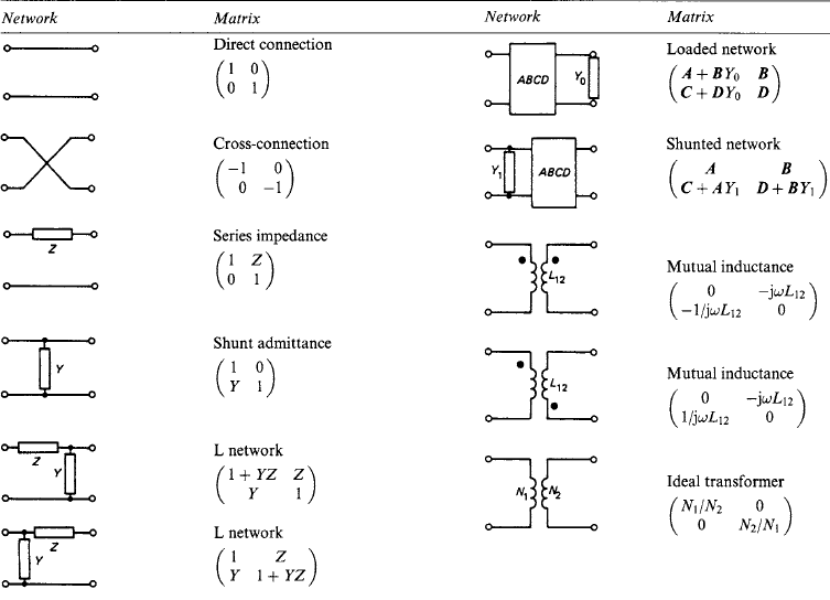
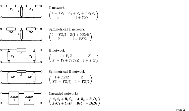
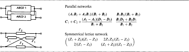
The values of the ABCD parameters, in matrix form,

are set out in Table 3.1 for a number of common cases.
3.2.5.4 Characteristic impedance
If the output terminals of a two-port are closed through an impedance V2/I2 = Z0, and if the input impedance V1/I1 is then also Z0, the quantity Z0 is the characteristic impedance. Consider a symmetrical two-port (A = D) so terminated: if V1/I1 is to be Z0 we have
which is Z0 for B/Z0 = CZ0. Thus the characteristic impedance is ![]() . The same result is obtainable from the input impedances with the output terminals first open circuited (I2 = 0) giving Zoc, then short circuited (V2 = 0) giving Zsc: thus
. The same result is obtainable from the input impedances with the output terminals first open circuited (I2 = 0) giving Zoc, then short circuited (V2 = 0) giving Zsc: thus
3.2.5.5 Propagation coefficient
The parameters ABCD are functions of frequency, and Z0 is a complex operator. For the Z0 termination of a symmetrical two-port (for which A2 − BC = 1) the input/output voltage or current ratio is
The magnitude of V1 exceeds that of V2 by the factor exp(α) and leads it by the angle β, where α is the attenuation coefficient, β is the phase coefficient and the combination γ = α + jβ is the propagation coefficient.
3.2.5.6 Alternative two-port parameters
There are other ways of expressing two-port relationships. For generality, both terminal voltages are taken as applied and both currents are input currents. With this convention it is necessary to write −I2 for I2 in the general parameters so far discussed. The mesh-current and node-voltage methods (Section 3.2.4) give V1 = I1z11 + I2z12, etc., and I1 = V1y11 + V2y12, etc., respectively. A further method relates V1 and I2 to I1 and V2 by hybrid (impedance and admittance) parameters. The four relationships are then obtained as follows:
If the networks are passive, then z12 = z21, y12 = y21 and h12 = −h21. If, in addition, the networks are symmetrical, then A = D, z11 = z22 and y11 = y22. If the networks are active (i.e. they contain sources), then reciprocity does not apply and there is no necessary relation between the terms of the 2 × 2 matrix.
3.2.6 Network topology
In multibranch networks the solution process is aided by representing the network as a graph of nodes and interconnections. The topology is the scheme of interconnections. A network is planar if it can be drawn on a closed spherical (or plane) surface without cross-overs. A non-planar network cannot be so drawn: a single cross-over can be eliminated if the network is drawn on a more complicated surface resembling a doughnut, and more cross-overs require closed surfaces with more holes.
The nomenclature employed in topology is as follows.
Graph: A diagram of the network showing all the nodes, with each branch represented by a plain line.
Tree: Any arrangement of branches that connects all nodes together without forming loops. A tree branch is one branch of such a tree.
Cut set: A set of branches comprising one tree branch, the other branches being tree links. A cut set dissociates two main portions of a network in such a way that replacing any one element destroys the dissociation.
Before setting up the equations for network solution, some guide is necessary in forming the proper number of independent equations. Given the network (a) in Figure 3.10, the first step is to draw the graph (b). Two of its possible trees are shown in (c). The trees are then used to set up the equations.
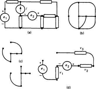
3.2.6.1 Network equations
Voltage: The network diagram for the upper tree in Figure 3.10(c) is drawn in (d). Specifying the tree-branch voltages specifies also the voltages across the links. It is convenient to choose r as a reference node, leaving n = 6 independent nodes requiring n = 6 voltage equations.
3.2.6.2 Ports
It is often helpful to place the sources outside the network and to regard their connections to the (now passive) remainder as ports. Again, branches of interest can be taken outside and used to terminate ports, as in Figure 3.11.
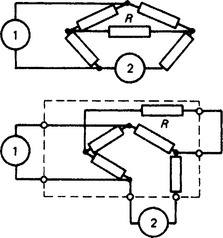
A multiport network (Figure 3.12) has the following characteristic definitions:
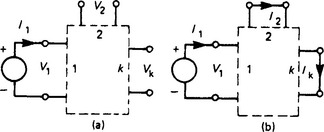
(a) All ports but one are open-circuited: a voltage V1 is applied to port 1 and a current I1 flows into it. Then V1/I1 is the open-circuit (o.c.) driving-point impedance at port 1, Vk/I1 is the o.c. transfer impedance from port 1 to port k, and Vk/V1 is the o.c. voltage ratio of port k to port 1.
(b) All ports but one are short circuited: a current I1 (requiring a voltage V1) is fed in at port 1. Then I1/V1 is the short-circuit (s.c.) driving-point admittance at port 1, Ik/V1 is the s.c. transfer admittance from port 1 to port k, and Ik/I1 is the s.c. current ratio of port k to port 1.
3.2.7 Steady-state d.c. networks
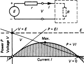
The steady state implies that energy storage in electric and magnetic fields does not change, and only the resistance is significant. In Figure 3.13 a source of constant e.m.f. E and internal resistance r provides a current I at terminal voltage V to a network represented by an equivalent resistance R. On open circuit (R = ∞), I = 0 and V = E. As R is reduced the source provides a current I = E/(R + r) = (E − V)/r. The greatest output power P = VI occurs for the condition R = r, further reduction of R reduces the network power, down to a short-circuit condition for R = 0 and V = 0 when the source power is dissipated entirely in r. The maximum-power condition is utilised only with sources whose power capability is very small.
3.2.8 Steady-state a.c. networks
An a.c. flows alternately in the specified positive direction and then in the negative direction in a circuit, repeating this cycle continuously. A graph of current or voltage to a time base shows the waveform as a succession of instantaneous values. In general there will be a maximum or peak value in both positive and negative half-periods where the current or voltage is greatest. The time for one complete cycle is the period T. The number of periods per second is the frequency f = 1/T.
An a.c. is produced by an alternating voltage. Two such quantities may have a difference of phase, to which a precise meaning can be given only when the quantities are both sinusoidal functions of time.
3.2.8.1 Root-mean-square (r.m.s.) value
The numerical value assigned to an a.c. or voltage is normally defined in terms of mean power in a pure resistor. An a.c. of 1 A is that which produces heat energy at the same mean rate as a direct current of 1 A in the same non-reactive resistor. If i is the instantaneous value of an a.c. in a pure resistance R, the heat developed in a time element dt is dw = i2R dt. The mean rate (i.e. the mean power) over a complete period T is
and I is the r.m.s. value of the current. An alternating voltage is defined in a similar way; the instantaneous power is v2/R, and the mean is V2/R where V is the square root of the mean v2.
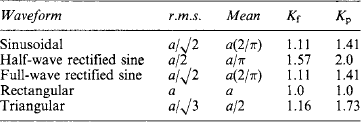
In some cases the peak or the mean value of the current or voltage waveform is more significant, particularly with asymmetric, pulse or rectified waveforms. The value to be understood by the term ‘mean’ is then obvious. In the case of a symmetrical wave, the half-period mean value is intended, as the mean over a complete period is zero. Table 3.2 gives the mean and r.m.s. values for a number of typical waveforms, together with the values of
The techniques developed for the solution of steady-state a.c. networks depend on the waveform. One technique applies to purely sinusoidal quantities, another to periodic but non-sinusoidal waveforms. In each case the network is assumed to be linear so that the principle of superposition is valid.
3.2.9 Sinusoidal alternating quantities
For pure sinusoidal waveforms, a current can be expressed as a function of time, i=im sin(2πft) = im sin(ωt), completing f cycles in 1 s with a period T = 1/f The quantity 2πf is contracted to ω, the angular frequency. The sine-wave shape has the advantages that (i) it is mathematically simple and its integral and differential are both cosinusoidal, (ii) it is a waveform desirable for power generation, transmission and utilisation, and (iii) it lends itself to phasor and complexor representation.
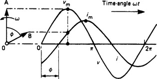
The graph of a sinusoidal current or voltage of frequency f can be plotted to a time-angle base ωt by use of trigonometric tables. Alternatively it can be represented by the projection of a line of length equal to the peak value and rotating counter-clockwise at angular speed ω about one end O. A stationary line can represent the sine wave, particularly in relation to other sine waves of the same frequency but ‘out of step’. Two such waves, say v and i with peak values vm and im, respectively, can be written
and drawn as in Figure 3.14, the phase difference or phase angle between them being φ rad. Then two lines, OA and OB, having an angular displacement φ, can represent the two waves in peak magnitude and relative time phase.
Although developed from rotating lines of peak-value length, it is more convenient to change the scale and treat the lengths as r.m.s. values. The processes of addition and subtraction of r.m.s. values are performed as if the lines were co-planar vector forces in mechanics. Physically, however, the lines are not vectors: they substitute for scalar quantities, alternating sinusoidally with time. They are termed phasors. Certain associated quantities, such as impedance, admittance and apparent power, can also be represented by directed lines, but as they are not sinusoids they are termed complexors or complex operators. Both phasors and complexors can be dealt with by application of the theory of complex numbers. The definitions concerned are listed below.
Complexor A generic term for a non-vector quantity expressed as a complex number.
3.2.9.1 Complexor algebra
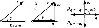
The four arithmetic processes for complexors are applications of the theory of complex numbers. Complexor a in Figure 3.15 can be expressed by its magnitude a and its angle θ with respect to an arbitrary ‘datum’ direction (here taken as horizontal) as the simple polar form a = a ∠ θ. Alternatively it can be written as a = p + jq, the rectangular form, in terms of its projection p on the datum and q on a quadrature axis at right angles thereto: q (as a scalar magnitude along the datum) is rotated counter-clockwise by angle 1/2π rad (90°) by the operator j. Two successive operations by j (written as j2) give a rotation of π rad (180°), making the original +q into −q, in effect a multiplication by −1. Three operations (j3) give − jq and four give +q. Thus any complexor can be located in the complex datum-quadrature plane. Further obvious forms are the trigonometric, a = a(cos θ + j sin θ), and the exponential, a = a exp(jθ). Summarising, the four descriptions are:
Consider complexors a = p + jq = a ∠ α and b = r + js = b ∠ β. The basic manipulations are:

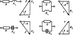
3.2.9.2 Impedance and admittance operators
Sinusoidal voltages and currents can be represented by phasors in the expressions V = IZ = I/Y and I = VY = V/Z. Current and voltage phasors are related by multiplication or division with the complex operators Z and Y. Series resistance R and reactance jX can be arranged as a right-angled triangle of hypotenuse ![]() and the angle between Z and R is θ = arctan(X/R). The relation between Z and Y for the same series network elements with Z = R + jX is
and the angle between Z and R is θ = arctan(X/R). The relation between Z and Y for the same series network elements with Z = R + jX is
where G and B are defined in terms of R, X and Z. The series components R and X become parallel branches in Y, one a pure conductance, the other a pure susceptance. Further, a positive-angled impedance has, as inverse equivalent, a negative-angled admittance (Figure 3.16).
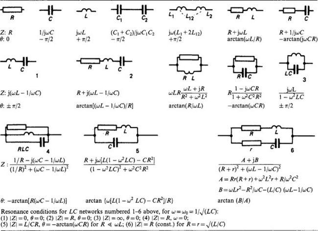
The impedance and phase angle of a number of circuit combinations are given in Table 3.3.
Impedance and admittance loci: If the characteristics of a device or a circuit can be expressed in terms of an equivalent circuit in which the impedances and/or admittances vary according to some law, then the current taken for a given applied voltage (or the voltage for a given current) can be obtained graphically by use of an admittance or impedance locus diagram.
In Figure 3.17(a), let OP represent an impedance Z = R + jX and OQ the corresponding admittance Y = G − jB. Point Q is obtained from P by finding first the geometric inverse point Q′ such that OQ′ = 1/OP to scale, and then reflecting OQ′ across the datum line to give OQ and thus a reversed angle –θ, a process termed complexor inversion. If Z has successive values Z1, Z2, …, on the impedance locus, the corresponding admittances Y1, Y2, …, lie on the admittance locus. The inversion process may be point-by-point, but in many cases certain propositions can reduce the labour:
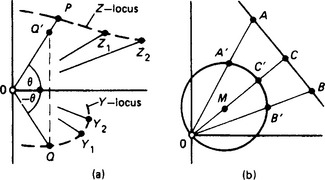
(1) Inverse of a straight line–the geometric inverse of a straight line AB about a point O not on the line is a circle passing through O with its centre M on the perpendicular OC from O to AB (Figure 3.17(b)). Then A′ is the geometric inverse of A, B′ of B, etc.; also, A is the inverse of A′, B of B′, etc.
(2) Inverse of a circle–from the foregoing, the geometric inverse of a circle about a point O on its circumference is a straight line. If, however, O is not on the circumference, the inverse is a second circle between the same tangents; but the distances OM and OM′ from the origin O to the centres M and M′ of the circles are not inverses of each other.
The choice of scales arises in the inversion process: for example, the inverse of an impedance Z = 50 ∠ 70° Ω is Y = 0.02 ∠ (−70°) S. It is usually possible to decide on a scale by taking a salient feature (such as a circle diameter) as a basis.
3.2.9.3 Power
The instantaneous power delivered to a load is the product of the instantaneous voltage v and current i. Let v = vm sin ωt and i = im sin(ωt − φ) as in Figure 3.18(a); then the instantaneous power is
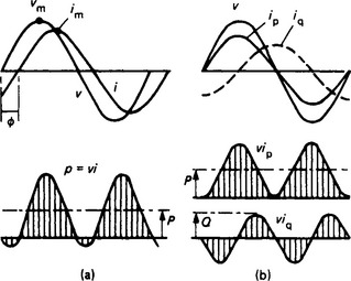
This is a quantity fluctuating at angular frequency 2Ω with, in general, excursions into negative power (i.e. that returned by the load to the source). Over an integral number of periods the mean power is
where V and I are r.m.s. values.
Now resolve i into the active and reactive components
as in Figure 3.18(b); then the instantaneous power can be written
Over a whole number of periods the average of the first term is
giving the average rate of energy transfer from source to load. The second term is a double-frequency sinusoid of average value zero, the energy flow changing direction rhythmically between source and load at a peak rate
The power conditions thus summarise to the following:
Active power P: The mean of the instantaneous power over an integral number of periods giving the mean rate of energy transfer from source to load in watts (W).
Reactive power Q: The maximum rate of energy interchange between source and load in reactive volt-amperes (var).
Apparent power S: The product of the r.m.s. voltage and current in volt-amperes (V-A).
Both P and Q represent real power. The apparent power S is not a power at all, but is an arbitrary product VI. Nevertheless, because of the way in which P and Q are defined, we can write
whence ![]() , a convenient combination of mean active power with peak power circulation.
, a convenient combination of mean active power with peak power circulation.
3.2.9.4 Resonance
A condition of resonance occurs when the load contains two forms of energy-storing element (L and C) such that, at the frequency of operation, the two energies are equal. The reactive power requirements are then satisfied internally, as the inductor releases energy at the rate that the capacitor requires it. The source supplies only the active power demand of the energy-dissipating load components, the load externally appearing to be purely resistive.
Acceptor resonance: The series RLC circuit in Figure 3.19(a) has, at angular frequency ω, the impedance Z = R + jX, where X is ωL-1/ωC, which for ![]() is zero. The impedance is then Z = R and the input current has a maximum I0 = V/R, conditions of acceptor resonance. Internally, large voltages appear across the reactive components, viz.
is zero. The impedance is then Z = R and the input current has a maximum I0 = V/R, conditions of acceptor resonance. Internally, large voltages appear across the reactive components, viz.
The terms L/R and 1/CR are the time constants of the reactive elements, and ω0L/R is the Q value of a practical inductor of inductance L and loss-resistance R. The Q value may be large (e.g. 100) for resonance at a high frequency.
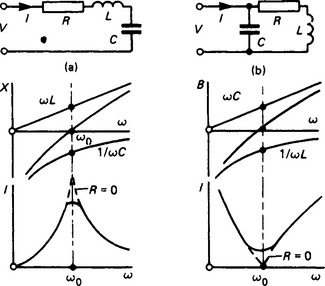
Rejector resonance: This occurs in a parallel combination of L and C, the energies circulating around the closed LC loop. If in Figure 3.19(b) the resistance R is zero, the terminal input admittance vanishes at angular frequency ![]() , with ω0C = 1/ω0L and an input susceptance B = 0. Where the circuit contains resistance R the resonance conditions are less definite. Three possible criteria are: (i)
, with ω0C = 1/ω0L and an input susceptance B = 0. Where the circuit contains resistance R the resonance conditions are less definite. Three possible criteria are: (i) ![]() , (ii) the input admittance is a minimum, and (iii) the input admittance is purely conductive. All three criteria are satisfied simultaneously in the simple acceptor circuit, but differ in rejector conditions; however, where resonance is an intended property of the circuit, the differences are small.
, (ii) the input admittance is a minimum, and (iii) the input admittance is purely conductive. All three criteria are satisfied simultaneously in the simple acceptor circuit, but differ in rejector conditions; however, where resonance is an intended property of the circuit, the differences are small.
Some expressions for resonance are given for six circuit arrangements in Table 3.3.
3.2.10 Non-sinusoidal alternating quantities
Periodic but non-sinusoidal currents occur: (i) with non-sinusoidal e.m.f. sources, (ii) with sinusoidal sources applied to non-linear loads, and (iii) with any combination of (i) and (ii).
3.2.10.1 Fourier series
Any univalued periodic waveform can be represented as a summation of sine waves comprising a fundamental, where frequency is that of the periodic occurrence, and a series of harmonic waves of frequency 2, 3, …, n times that of the fundamental. The Fourier series for a periodic function y = f(x) takes either of the following equivalent forms:
where c0 is a constant, ![]() and αn = arctan (an/bn). The coefficients of the terms are given by
and αn = arctan (an/bn). The coefficients of the terms are given by
These can be evaluated mathematically for simple cases. The work may sometimes be reduced by inspection: thus c0 = 0 for a wave symmetrical about the baseline; or only odd-order harmonics may be present.
3.2.10.2 Analysis
The series for a range of mathematically tractable waveforms are given in Table 1.10. For experimentally derived waveforms there are several methods, but none yields the amplitude of higher order harmonics without considerable labour, unless a computer program is available.
A particular harmonic, say the n th, may be found by superimposing n copies of the wave, displaced relatively by 2π/n, 4π/n, …, and adding the corresponding ordinates. The result is a wave of frequency n times that of the harmonic sought (with the addition, however, of harmonics of orders kn where k is an integer). The method gives also the phase angle αn.
A semi-graphical method is shown in Figure 3.20. The base of a complete period 2π is divided into m parts, the corresponding ordinates being y0, y1, y2, …, ym. Construct axes OA and OB; set out the radii y0 to ym (=y0) at angles 0, 2nπ/m, 4nπ/m, …, from the axis OA. Then project the extremities horizontally (p) and vertically (q), and take the sum of the two sets of projections with due regard to their sign. Then for the n th harmonic
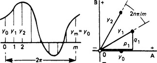
The labour is reduced if 2π/m is a simple fraction of 2π, for then some groups of radii are coincident.
3.2.10.3 Power
is obtained from the square root of the average squared value, resulting in
where ![]() , etc., are the r.m.s. values of the individual harmonic components. The r.m.s. voltage is obtained in a similar way.
, etc., are the r.m.s. values of the individual harmonic components. The r.m.s. voltage is obtained in a similar way.
Power: The instantaneous power p in a circuit with an applied voltage
is the product vi: this includes (i) a series of the form
all terms of which have a fundamental-period average ½ vnin cos φn; and (ii) a series of the form
which, over a fundamental period, averages zero. Power is circulated by a voltage and a current of different frequencies, but the circulation averages zero. The mean (active) power is therefore
where the capital letters denote component r.m.s. values. Thus the harmonics contribute power separately.
Power factor: The ratio of the active power P to the apparent power S is
This may be less than unity even with all phase angles zero if the ratio Vn/In is not the same for each component. Where the applied voltage is a pure sinusoid of fundamental frequency there can be no harmonic powers; the active power is P = V1/I1 cos φ1. Then
where ![]() , the distortion factor. The overall power factor is consequently δ cos φ1. This is typical of circuits containing non-linear elements.
, the distortion factor. The overall power factor is consequently δ cos φ1. This is typical of circuits containing non-linear elements.
3.2.11 Three-phase systems
A symmetrical m-phase system has m source e.m.f.s, all of the same waveform and frequency, and displaced 2π/m rad or 1/m period in time; m is most commonly 3, but is occasionally 6, 12 or 24.
Symmetric three-phase system: In Figure 3.21(a) the symmetric sinusoidal three-phase system has source e.m.f.s in phases A, B and C given by
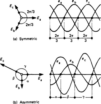
The instantaneous sum of the phase e.m.f.s (and also the phasor sum of the corresponding r.m.s. phasors Ea, Eb and Ec) is zero.
Asymmetric three-phase system: The asymmetric system in Figure 3.21(b) has, in general, unequal phase voltages and phase displacements. Such asymmetry may occur in machines with unbalanced phase windings and in power supply systems when faults occur; the usual method of dealing with asymmetry is described in section 3.2.12. Attention here is confined to the basic symmetric cases.
3.2.11.1 Phase interlinkage
While individual phase sources can be used separately, they are generated in the same machine and are normally interlinked. Using r.m.s. phasors, let the e.m.f. in a generator winding XY be such as to drive positive current out at X: then X is positive to Y and its e.m.f. EXY is represented by an arrow with its point at X. The e.m.f. EYX between terminals Y and X is therefore −EXY. Further, when two windings XN and YN have a common terminal N, the e.m.f.s are
Common phase interconnections are shown in Figure 3.22.
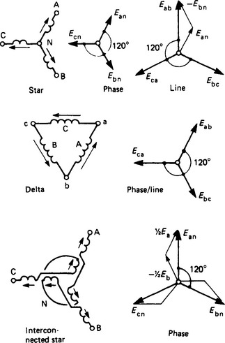
3.2.11.2 Star
Let the phase e.m.f.s be Ean, Ebn and Ecn with an arbitrary positive direction outward from the star-point N. Then the line e.m.f.s are
These are of magnitude ![]() times that of a phase e.m.f., and provide a symmetric three-phase system of line e.m.f.s, with Eab leading Ean by 30°. Thus
times that of a phase e.m.f., and provide a symmetric three-phase system of line e.m.f.s, with Eab leading Ean by 30°. Thus ![]() and It = IPh, the subscripts 1 and ph referring to line and phase quantities respectively.
and It = IPh, the subscripts 1 and ph referring to line and phase quantities respectively.
3.2.11.3 Delta
The line-to-line e.m.f. is that of the phase across which the lines are connected. The line current is the difference of the currents in the phases forming the line junction, so that the relations for symmetric loading are E1 = Eph and ![]() .
.
3.2.11.4 Interconnected star
A line-to-neutral e.m.f. comprises contributions from successive half-phases and sums to ![]() of a complete phase e.m.f. The line-to-line e.m.f. is 1 1/2 times the magnitude of a complete phase e.m.f. and the line current is numerically equal to the phase current.
of a complete phase e.m.f. The line-to-line e.m.f. is 1 1/2 times the magnitude of a complete phase e.m.f. and the line current is numerically equal to the phase current.
3.2.11.5 Power
The total power delivered to or absorbed by a polyphase system, be it symmetric and balanced or not, is the algebraic sum of the individual phase powers. Consider an m-phase system with instantaneous line currents i1, i2, …, im, the algebraic sum of which is zero by the Kirchhoff node law. Let the voltages of the input (or output) terminals, with reference to a common point X, be v1 − vx, v2 − vX, …, vm − vx; then the instantaneous powers will be (v1 − vx)i1, (v2 − vx)i2, …, (vm − vx)im, which together sum to the total instantaneous power p. There is no restriction on the choice of X; it can be any of the terminals, say M. In this case vm − vx = vm − vm = 0, and the power summation has only m-1 terms. The average power over a full period T is, therefore,
The first term of the sum in brackets represents the indication of a wattmeter with i1 in its current circuit and v1 − vm across its volt circuit, i.e. connected between terminals 1 and M. It follows that three wattmeters can measure the power in a three-phase four-wire system, and two in a three-phase three-wire system. Some of the common cases are listed below.
(1) Three-phase, four-wire, load unbalanced-The connections are shown in Figure 3.23(a). Wattmeters W1, W2 and W3 measure the phase powers separately. The total power is the sum of the indications:
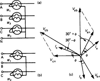
(2) Three-phase, four-wire, load balanced—with the connections shown in Figure 3.23(a), all the meters read the same. Two of the wattmeters can be omitted and the reading of the remaining instrument multiplied by 3.
(3) Three-phase, three-wire, load unbalanced—two wattmeters are connected with their current circuits in any pair of lines, as in Figure 3.23(b). The total power is the algebraic sum of the readings, regardless of waveform. A two-element wattmeter summates the power automatically; with separate instruments, one will tend to read reversed under certain conditions, given below.
(4) Three-phase, three-wire, load balanced—with sinusoidal voltage and current the conditions in Figure 3.23(c) obtain. Wattmeters W1 and W2 indicate powers P1 and P2 where
The total active power P = P1 + P2 is therefore
where cos φ is the phase power factor. The algebraic difference is P1 − P2 = V1I1 sin φ, whence the reactive power is given by
and the phase angle can be obtained from φ = arctan (Q/P). For φ = 0 (unity power factor) both wattmeters read alike; for φ = 60° (power factor 0.5 lag) W1 reads zero; and for lower lagging power factors W1 tends to read backwards.
The active power of a single phase has a double-frequency pulsation (Figure 3.18). For the asymmetric two-phase system under balanced conditions and a phase displacement of 90°, and for all symmetric systems with m = 3 or more, the total power is constant.
3.2.11.6 Harmonics
Considering a symmetrical balanced system of three-phase non-sinusoidal voltages, and omitting phase displacements (which are in the context not significant), let the voltage of phase A be
Writing ![]() and
and ![]() , respectively, for phases B and C, and simplifying, we obtain
, respectively, for phases B and C, and simplifying, we obtain
The fundamentals have a normal 2π/3 rad (120°) phase relation in the sequence ABC, as also do the 4th, 7th, 10th,…, harmonics. The 2nd (and 5th, 8th, 11th,…) harmonics have the 2π/3 rad phase relation but of reversed sequence ACB. The triplen harmonics (those of the order of a multiple of 3) are, however, co-phasal and form a zero-sequence set.
The relation ![]() in a three-phase star-connected system is applicable only for sine waveforms. If harmonics are present, the line- and phase-voltage waveforms differ because of the effective phase angle and sequence of the harmonic components. The n th harmonic voltages to neutral in two successive phases AB are vn sin nωt and
in a three-phase star-connected system is applicable only for sine waveforms. If harmonics are present, the line- and phase-voltage waveforms differ because of the effective phase angle and sequence of the harmonic components. The n th harmonic voltages to neutral in two successive phases AB are vn sin nωt and ![]() , and between the corresponding line terminals the n th harmonic voltage is 2vn sin n(1/3π). For triplen harmonics this is zero; hence no triplens are present in balanced line voltages because, in the associated phases, their components are equal and in opposition. In a balanced delta connection, again no triplens are present between lines: the delta forms a closed circuit to triplen circulating currents, the impedance drop of which absorbs the harmonic e.m.f.s.
, and between the corresponding line terminals the n th harmonic voltage is 2vn sin n(1/3π). For triplen harmonics this is zero; hence no triplens are present in balanced line voltages because, in the associated phases, their components are equal and in opposition. In a balanced delta connection, again no triplens are present between lines: the delta forms a closed circuit to triplen circulating currents, the impedance drop of which absorbs the harmonic e.m.f.s.
3.2.12 Symmetrical components
Figure 3.21(a) shows the sine waves and phasors of a balanced symmetric three-phase system of e.m.f.s of sequence ABC. The magnitudes are equal and the phase displacements are 2π/3 rad. In Figure 3.21(b), the asymmetric sine waveforms have also the sequence ABC, but they are of different magnitudes and have the phase displacements α, β and γ. Problems of asymmetry occur in the unbalanced loading of a.c. machines and in fault conditions on power networks. While a solution is possible by the Kirchhoff laws, the method of symmetrical components greatly simplifies analysis.
Any set of asymmetric three-phase e.m.f.s or currents can be resolved into a summation of three sets of symmetrical components, respectively of positive phase-sequence (p.p.s.) ABC, negative phase-sequence (n.p.s.) ACB, and zero phase-sequence (z.p.s.). Use is made of the operator a, resembling the 90° operator j (Section 3.2.9.1) but implying a counter-clockwise rotation of 2π/3 rad (120°). Thus
A symmetric three-phase system has only p.p.s. components
whereas an asymmetric system (Figure 3.24) comprises the three sets
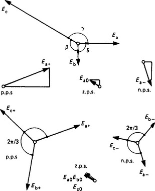
where the subscripts 0, + and − designate the z.p.s., p.p.s. and n.p.s. components, respectively. The p.p.s. and the n.p.s. components sum individually to zero. Therefore, if the originating phasors Ea, Eb, Ec also sum to zero there are no z.p.s. components; if they do not, their residual is the sum of the three z.p.s. components.
The asymmetrical phasors have now been reduced to the sum of three sets of symmetrical components:
The components are evaluated from the arbitrary identities
Figure 3.24 is drawn for an asymmetric system with voltages Ea = 200, Eb = 100 and Ec = 400V, and phase-displacement angles δ = 90°, β=120° and γ=150°. In phasor terms,
The summation Ea0 + Ea+ + Ea- = 200 + j0 = Ea. The p.p.s and n.p.s. components of Eb and Ec are readily obtained.
3.2.12.1 Power
In linear networks there is no interference between currents of different sequences. Thus p.p.s. voltages produce only p.p.s. currents, etc. The total power is therefore
This is equivalent to the more obvious summation of phase powers
Symmetrical-component techniques are useful in the analysis of power-system networks with faults or unbalanced loads: an example is given in Section 3.3.4. Machine performance is also affected when the machine is supplied from an asymmetric voltage system: thus in a three-phase induction motor the n.p.s. components set up a torque in opposition to that of the (normal) p.p.s. voltages.
3.2.13 Line transmission
Networks of small physical dimensions and operated at low frequency are usually considered to have a zero propagation time; a current started in a closed circuit appears at every point in the circuit simultaneously. In extended circuits, such as long transmission lines, the propagation time is significant and cannot properly be ignored.
The basics of energy propagation on an ideal loss-free line are discussed in another section. Propagation takes place as a voltage wave v accompanied by a current wave i such that v/i = z0 (the surge impedance) travelling at speed u. Both z0 and u are functions of the line configuration, the electric and magnetic space constants ε0 and μ0, and the relative permittivity and permeability of the medium surrounding the line conductors. At the receiving end of a line of finite length, an abrupt change of the electromagnetic-field pattern (and therefore of the ratio v/i) is imposed by the discontinuity unless the receiving-end load is z0, a termination called the natural load in a power line and a matching impedance in a telecommunication line. For a non-matching termination, wave reflection takes place with an electromagnetic wave running back towards the sending end. After many successive reflections of rapidly diminishing amplitude, the system settles down to a steady state determined by the sending-end voltage, the receiving-end load impedance and the line parameters.
3.2.13.1 A.c. power transmission
The steady-state condition considered is the transfer of a constant balanced apparent power per phase from a generator at the sending end (s) to a load at the receiving end (r) by a sinusoidal voltage and current at a frequency f = ω/2π. The line has uniformly distributed parameters: a conductor resistance r and a loop inductance L effectively in series, and an insulation conductance g and capacitance C in shunt, all per phase and per unit length. The series impedance, shunt admittance and propagation coefficient per unit length are z = r + j ωL, y = g + j ωC and ![]() . The solution for the receiving-end terminal conditions is in terms of
. The solution for the receiving-end terminal conditions is in terms of ![]() and its hyperbolic functions as a two-port:
and its hyperbolic functions as a two-port:
Using the hyperbolic series (Section 1.2.2) and writing ![]() , we obtain for a symmetrical line
, we obtain for a symmetrical line
The significance of the higher powers of YZ depends on: (i) the line configuration, (ii) the properties of the ambient medium, and (iii) the physical length of the line in terms of the wavelength λ = u/f For air-insulated overhead lines the inductance is large and the capacitance small: the propagation velocity approximates to u = 3 × 10⁵ km/s (corresponding to a wavelength λ = 6000 km at 50 Hz), with a natural load z0 of the order of 400–500 Ω. Cable lines have a low inductance and a large capacitance: the permittivity of the dielectric material and the presence of armouring and sheathing result in a propagation velocity around 200 km/s, a surge impedance below 100 Ω, and the possibility (in high-voltage cables) that the charging current may be comparable with the load current if the cable length exceeds 25–30 km.
For balanced three-phase power transmission, the general equations are applied for the line-to-neutral voltage, line current and phase power factor. Phasor diagrams for the load and no-load (Ir = 0) receiving-end conditions for an overhead-line transmission are shown in Figure 3.25, with Vr as datum. On no load, Vs = VrA, and as A has a magnitude less than unity and a small positive angle α, the phasor VrA is smaller than Vr and leads it by angle α: thus Vr > Vs, the Ferranti effect. For the loaded condition, IrB is added to VrA to give Vs. Similarly VrC is added to IrD to obtain IS.
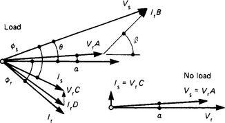
The product VrIr = Ir(Vs − VrA) is the receiving-end complex apparent power Sr. Let Vs lead Vr by angle θ; then the receiving-end load has the active and reactive powers Pr and Qr given by
where α and β are the angles in the complexors A and B. The importance of B (roughly the overall series impedance) is clear.
Line chart: Operating charts for a transmission circuit can be drawn to relate graphically Vs, Vr, Pr and Qr, using the appropriate overall ABCD parameters (e.g. with terminal transformers included).
Receiving-end chart: A receiving-end chart gives active and reactive power at the receiving end for Vr constant (Figure 3.26(a)). The co-ordinates (x, y) and the radius (r) of the constant-voltage circles are
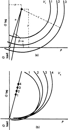
where A and B are scalar magnitudes, and α and β the angles in A and B. For a given Vr the chart comprises a family of concentric circles, each corresponding to a particular Vs. If a given receiving-end load is located by its active and reactive power components, Vs is obtained from the corresponding Vs circle.
Sending-end chart For a given Vs the sending-end chart comprises a family of circles as shown in Figure 3.26(b), each circle corresponding to a particular Vr. Load points outside the envelope of these circles cannot be supplied at the Vs for which the chart is drawn.
3.2.13.2 Short line
For an overhead interconnector line the capacitive shunt admittance is neglected, reducing the general parameters to A = D = 1, B = Z = R + jX and C = 0. The operating conditions are those in Figure 3.27, with a receiving-end voltage Vr (taken as reference phasor), a sending-end voltage Vs and a load current I at a lagging phase angle φ with respect to Vr and having active and reactive components respectively Ip and Iq. Then
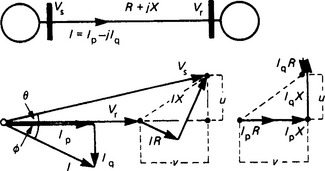
To a close approximation, v is the difference of the voltages Vs and Vr, while u determines their phase difference (or transmission angle). The regulation and angle are therefore v/Vs p.u. and θ = arctan(u/Vs) rad.
Suppose that Vr = Vs; then v = 0 giving Iq = −Ip(R/X), and u = IpX[1 + (R/X)2] giving θ = arctan(Ip/Vs) [1 + (R/X)2]. The consequences are that (i) for a receiving-end active power P the load must be able to absorb a leading reactive power Q = P(R/X), and (ii) the transmission angle is determined largely by X. If R/X = 0.5, typical of an overhead line, then Q = 0.5P and θ = arctan[1.25 X(IP/VS)]. With interconnector cables the R/X ratio is usually greater than unity and shunt capacitance current is no longer negligible.
Independent adjustment of Vs and Vr is not feasible, and effective load control requires adjustment of v (e.g. by transformer taps) and of u (e.g. by quadrature boosting).
3.2.14 Network transients
Energy cannot be instantaneously converted from one form to another, although the time needed for conversion can be very short and the conversion rate (i.e. the power) high. Change between states occurs in a period of transience during which the system energies are redistributed in accordance with the energy-conservation principle (Section 1.3.1). For example, in a simple series circuit of resistance R, inductance L and capacitance C connected to a source of instantaneous voltage v, the corresponding rates of energy input, dissipation (in R) and storage (in L and C) are related by
Dividing by the common current i and writing the capacitor charge q as the time-integral of the current gives the voltage equation
and any changes in the parameters or in the applied voltage demand changes in the distribution of the circuit energy. The integro-differential equation can be solved to yield both steady-state and transient conditions.
In practical circuits the system may be too complex for such a direct solution; the following methods may then be attempted:
(1) formal mathematics for simple cases with linear parameters;
(2) simplification, e.g. by linearising parameters or by neglecting second-order terms;
(3) writing a possible solution based on the known physical behaviour of the system, with a check by differentiation;
(4) setting up a model system on an analogue computer; or
(5) programming a digital computer to give a solution by iteration.
3.2.14.1 Classification
Where the system has only one energy-storage component, single-energy transients occur. Where two (or more) different storages are concerned, the transient has a double-(or multiple-) energy form. Transients may occur in the following circumstances.
(1) Initiation—a system, initially dead, is energised.
(2) Subsidence—an initially energised system is reduced to a zero-energy condition.
(3) Transition—a change from one state to another, where both states are energetic.
(4) Complex—the superposition of more than one disturbance.
(5) Relaxation—transition between states that, when reached, are themselves unstable.
Further distinctions can be made, e.g. between linear and non-linear parameters, neglect or otherwise of propagation time within the system, etc. Attention here is mainly confined to simple electric networks with constant parameters and, by analogy (Section 1.3.1), to corresponding mechanical systems.
3.2.14.2 Transient forms
During transience, the current i for an impressed voltage stimulus v(t) is considered to be the superposition of a transient component it and a final steady-state current is, so that at any instant i = is + it. Alternatively, the voltage v for an impressed current stimulus i(t) is the summation v = vs + vt. The quantities is or vs are readily derived by applying the appropriate steady-state technique. The form of it or vt is characteristic of the system itself, is independent of the stimulus and comprises exponential terms k exp(λt) where k depends on the boundary conditions. This is the case because of the fixed proportionality between the stored energy 1/2 Li2 and the rate of energy dissipation Ri2 in an RL circuit; and similarly for 1/2 Cv2 and v2/R in an RC circuit. Hence the transient form can be obtained from a case in which the final steady state is of zero energy, i.e. a subsidence transient.
The subsidence transient in a single-energy (first-order) system having the general equation dy/dt + ay = 0 can be found by substituting λ for d/dt to give λy + ay = 0, whence λ = −a. Then the solution is
a simple exponential decay as in Figure 1.2 of Section 1.2.2. For a double-energy (second-order) system the basic equation is
The quadratic in λ has two roots, λ1 and λ2, and the solution has a pair of exponential terms that depend on the relation between a and b. For a multiple-energy (n th-order) system there will be n roots. From Section 1.2.2 it will be seen that exponential terms can represent oscillatory as well as decay forms of response.
Single-energy system: Consider the RL circuit shown in Figure 3.28, subsequent to closure of the switch at t = 0. The transient current form is obtained from L(di/dt) + Ri = 0, or Lλi + Ri = 0, giving λ = −R/L. Then
where T = L/R is the time-constant. The final steady-state current depends on the source voltage v. In Figure 3.28(a) with v = V, a constant direct voltage, is = V/R. Immediately after switching, with t = 0+, the current i is still zero because the inductance prevents any instantaneous rise. Hence
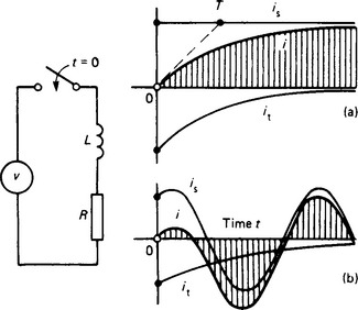
so that k = −(V/R). From t = 0 the current is, therefore,
The two terms and their summation are shown in Figure 3.28(a).
If, as in Figure 3.28(b), the source voltage is sinusoidal expressed by v = vm sin(ωt − α) and again switching occurs at t = 0, the form of the transient current is unchanged, but the final steady-state current is
where ![]() and φ = arctan(ωL/R). At t = 0+
and φ = arctan(ωL/R). At t = 0+
which gives k = −(vm/A) sin(−α−φ). The final steady-state and transient current components are shown in Figure 3.28(b) with their resultant. Initially the current is asymmetric, but subsequently the decay of it allows the current to approach the steady-state condition.
If ωL ![]() R, then approximately φ = ½π. Let the switch be closed at v = 0 for which α = 0. Then the current is
R, then approximately φ = ½π. Let the switch be closed at v = 0 for which α = 0. Then the current is
which raises i to twice the normal steady-state peak when t reaches a half-period: this is the doubling effect. However, if the switch is closed at a source-voltage maximum, the current assumes its steady-state value immediately, with no transient component.
Summary for an RL circuit: The transient current has a decaying exponential form, with a value of k such that, when it is added to the final steady-state current, the initial current flowing in the circuit at t = 0 is obtained. (In both of the cases in Figure 3.28 the initial current is zero.) Thus if the initial circuit current is 10 A and the final current is 25 A, the value of k is − 15 A.
For the CR circuit in Figure 3.29, the form of the transient is found from Ri + q/C = 0; differentiating, we obtain
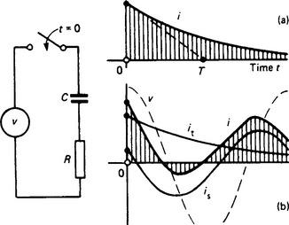
from which λ = −1/CR = −1/T, where T = CR is the time-constant. Thus i1 = k exp(−t/T). With the capacitor initially uncharged and a source direct voltage V switched on at t = 0,
As this must be V/R at t = 0+, then k = V/R, as shown in Figure 3.29(a). In Figure 3.29(b) the initiation of a CR circuit with a sine voltage is shown.
Summary for an RC circuit: The transient current is a decaying exponential k exp(−t/T). The initial current is determined by the voltage difference between the voltage applied by the source and that of the capacitor. (In Figure 3.29 the capacitor is in each case uncharged.) If this p.d. is V0, then the initial current is V0/R.
Double-energy system: A typical case is that of a series RLC circuit. The transient form is obtained from L(di/dt) + Ri + q/C = 0, differentiated to
Thus λ2 + (R/L)λ + 1/LC = 0 is the required equation, with the roots
The resulting transient depends on the sign of the quantity in parentheses, i.e. on whether R/2L is greater or less than ![]() . Four waveforms are shown in Figure 3.30.
. Four waveforms are shown in Figure 3.30.
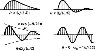
(1) Roots real: ![]() . The transient current is unidirectional and results from two simple exponential curves with different rates of decay.
. The transient current is unidirectional and results from two simple exponential curves with different rates of decay.
(2) Roots equal: ![]() . This has more mathematical than physical interest, but it marks the boundary between unidirectional and oscillatory transient current.
. This has more mathematical than physical interest, but it marks the boundary between unidirectional and oscillatory transient current.
(3) Roots complex: ![]() . The roots take the form −α± jωn, and the transient current oscillates with the interchange of magnetic and electric energies respectively in L and C; but the oscillation amplitude decays by reason of dissipation in R. With R = 0 the oscillation persists without decay at the undamped natural frequency
. The roots take the form −α± jωn, and the transient current oscillates with the interchange of magnetic and electric energies respectively in L and C; but the oscillation amplitude decays by reason of dissipation in R. With R = 0 the oscillation persists without decay at the undamped natural frequency ![]() .
.
Pulse drive: The response of networks to single pulses (or to trains of such pulses) is an important aspect of data transmission. An ideal pulse has a rectangular waveform of duration (‘width’) tp. It can be considered as the resultant of two opposing step functions displaced in time by tp as in Figure 3.31(a).
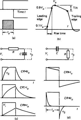
In practice a pulse cannot rise and fall instantaneously, and often the amplitude is not constant (Figure 3.31(b)). Ambiguity in the precise position of the peak value Vp makes it necessary to define the rise time as the interval between the levels 0.1 Vp and 0.9 Vp. The tilt is the difference between Vp and the value at the start of the trailing edge, expressed as a fraction of Vp.
The response of the output network to a voltage pulse depends on the network characteristics (in particular its time-constant T) and the pulse width tp. Consider an ideal input voltage Vi of rectangular waveform applied to an ideal low-pass series network (Figure 3.31(c)), the output being the voltage v0 across the capacitor C. Writing p for d/dt, then
where T= CR is the network time-constant. This represents an exponential growth v0 = Vi[1 -exp(−t/T)] over the interval tp. The trailing edge is an exponential decay, with t reckoned from the start of the trailing edge. Three typical responses are shown. For CR ![]() tp the output voltage reaches Vi; for CR > tp the rise is slow and does not reach Vi; for CR
tp the output voltage reaches Vi; for CR > tp the rise is slow and does not reach Vi; for CR ![]() tp the rise is almost linear, the final value is small and the response is a measure of the time-integral of Vi.
tp the rise is almost linear, the final value is small and the response is a measure of the time-integral of Vi.
With C and R interchanged as in Figure 3.31(d) to give a high-pass network, the whole of Vi appears across R at the leading edge, falling as C charges. Following the input pulse there is a reversed v0 during the discharge of the capacitor. The output/input voltage relation is given by
For CR ![]() tp the response shows a tilt; for CR
tp the response shows a tilt; for CR ![]() tp the capacitor charges rapidly and the output v0 comprises positive- and negative-going spikes that give a measure of the time-differential of Vi.
tp the capacitor charges rapidly and the output v0 comprises positive- and negative-going spikes that give a measure of the time-differential of Vi.
3.2.14.3 Laplace transform method
Application of the Laplace transforms is the most usual method of solving transient problems. The basic features of the Laplace transform are set out in Section 1.2.7 and Table 3.4, which gives transform pairs. The advantages of the method are that: (1) any stimulus, including discontinuous and pulse forms, can be handled, (2) the solution is complete with both steady-state and transient components, (3) the initial conditions are introduced at the start, and (4) formal mathematical processes are avoided.
Table 3.4
System transfer functions [the relation f2(t)/f1(t) of output to input quantity in terms of the Laplace transform F2(s)/F1(s)]
Consider the system in Figure 3.28(a). The applied direct voltage V has the Laplace transform V(s) = V/s; the operational impedance of the circuit is Z(s) = R + Ls. Then the Laplace transform of the current is
The term V/L is a constant unaffected by transformation. The term in s is almost of the form a/s(s + a). So, if we write
where a = R/L = 1/τ, the inverse Laplace transform gives
which is the complete solution. More complex problems require the development of partial fractions to derive recognisable transforms which are then individually inverse-transformed to give the terms in the solution of i(t).
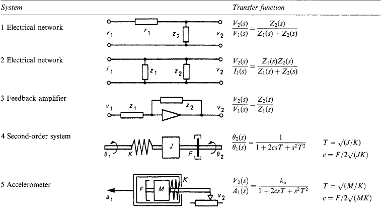
3.2.15 System functions
It is characteristic of linear constant-coefficient systems that their operational solution involves three parts: (i) the excitation or stimulus, (ii) the output or response and (iii) the system function. Thus in the relation I(s) = V(s)/Z(s) for the current in Z resulting from the application of V, 1/Z(s) is the system function relating voltage to current. For the simple electrical system shown in Figure 3.32(a) the system function Y(s) relating V(s) to I(s) in I(s) = V(s) Y(s) is Y(s) = 1/(R +Ls + 1/Cs). Different functions could relate the capacitor charge or the magnetic linkage in the inductor to the transform V(s) of the stimulus v(t).
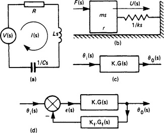
The mechanical analogue (Figure 3.32(b)) of this electrical system, as indicated in Section 1.3.1, has a system transfer function to relate force f(t) to velocity u(t) of the mass m and one end of the spring of compliance k in the presence of viscous friction of coefficient r. Then F(s) and U(s) are the transforms of f(t) and u(t), and the operational ‘mechanical impedance’ has the terms ms, 1/ks and r. In general, an input θi(s) and an output θo(s) are related by a system transfer function KG(s) (Figure 3.32(c)), where K is a numerical or a dimensional quantity to include amplification or the value of some physical quantity (such as admittance). The transform of the integro-differential equation of variation with time is expressed by the term G(s). The system is then represented by the block diagram in Figure 3.32(c); i.e. θo(s)/θi(s) = KG(s).
A number of typical system transfer functions for relatively simple systems are given in Table 3.4.
The output of one system may be used as the input to another. Provided that the two do not interact (i.e. the individual transfer functions are not modified by the connection) the overall system function is the product [K1G1(s)] × [K2G2(s)] of the individual functions. If the systems are paralleled and their outputs are additively combined, the overall function is their sum.
3.2.15.1 Closed-loop systems
In Figure 3.32, parts (a), (b) and (c) are open-loop systems. However, the output can be made to modify the input by feedback through a network KfGf(s) as in (d). The signal
is combined with θi(s) to give the modified input.
For positive feedback, the resultant input is σ(s) = θi(s) + θf(s), and the effect is usually to produce instability and oscillation.
For negative feedback, the resultant input is the difference ε(s) = θi(s) − θf(s), an ‘error’ signal. With the main system KG(s) now relating ε and θo, the output/input relation is
Suppose that there is unity feedback KfGf(s) = 1, then if KG (s) is large
and the output closely follows the input in magnitude and wave shape, a condition sought in servo-mechanisms and feedback controls.
3.2.15.2 System performance
In general, a system function takes the form numerator/denominator, each a polynomial in s, relating response to input stimulus. Two forms are
The response depends both on the system and on the stimulus. Performance can be studied if simple formalised stimuli (e.g. step, ramp or sinusoidal) are assumed; an exponential stimulus is even more direct because (in a linear system) the transient and steady-state responses are then both exponential. With the system function expressed in terms of the complex frequency s = σ + jω it is necessary to express the stimulus in similar terms and to evaluate the response as a function of time by inverse Laplace transformation. The response in the frequency domain (i.e. the output/input relation for sustained sinusoidal stimuli over a frequency range) is obtained by taking s = jω and solving the complexor KG(jω). Another alternative is to derive the poles (p) and zeroes (z) in equation (3.2) above.
Thus there are several techniques for evaluating system functions. Some are graphical and give a concise representation of the response to specified stimuli.
3.2.15.3 Poles and zeros
In equation (3.2), the numbers z are the values of s for which KG (s) = 0; for, if s is set equal to z1 or z2, …, the numerator has a zero term as a factor. Similarly, if s is set equal to p1 or p2, …, there is a zero factor in the denominator and KG(s) is infinite. Then the z terms are the zeros and the p terms are the poles of the system function. Except for the term bm/an, the system function is completely specified by its poles and zeros.
Consider the network of Figure 3.33, the system function required being the output voltage v0 in terms of the input voltage vi. This is the ratio of the paralleled branches R2L2C to the whole impedance across the input terminals. Algebra gives
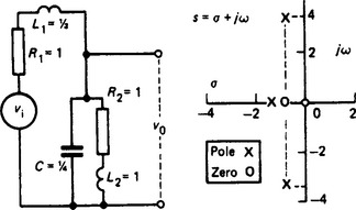
by factorising numerator and denominator. Thus there is one zero for s=−1. There are three poles, with s = −1.36, and −0.82 ± j3.33. These are plotted on the complex s-plane in Figure 3.33. Poles on the real axis σ correspond to simple exponential variations with time, decaying for negative and increasing indefinitely for positive values. Poles in conjugate pairs on the jω axis correspond to sustained sinusoidal oscillations. If the poles occur displaced from the origin and not on either axis, they refer to sinusoids with a decay or a growth factor, depending on whether the term σ is negative or positive.
3.2.15.4 Harmonic response
This is the steady-state response to a sinusoidal input at angular frequency ω. When a sine signal input is applied to a linear system, the steady-state response is also sinusoidal and is related to the input by a relative magnitude M and a phase angle α. The system function is KG(jω).
Consider again the network of Figure 3.33. Writing s = jω and simplifying gives the phasor expression for Vo/Vo as
Plots of |M| and ∠ α are shown in Figure 3.34(a). For ω = 0 the network is a simple voltage divider with Vo/Vi = 0.5 and a phase angle α = 0. For ω = ∞, the terminal capacitor effectively short circuits the output terminals so that V0/Vi = 0. At intermediate frequencies the gain |M| rises to a peak at ω = 3.3 rad/s and thereafter falls toward zero. The phase angle α is small and positive below ω = 1, being always negative thereafter, to become −180° at infinite frequency.
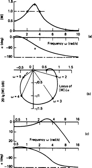
Nyquist diagram The Nyquist diagram is a polar plot of |M| ∠ α over the frequency range (Figure 3.34(b)), for an input Vi = 1 + j0. The plot is particularly useful for feedback systems. If the open-loop transfer function is plotted, and in the direction of increasing ω it encloses the point (−1 + j0), then when the loop is closed the system will be unstable as the output is more than enough to supply a feedback input even when Vi = 0. The Nyquist criterion for stability is therefore that the point (-1 + j0) shall not be enclosed by the plot.
Bode diagram The Bode diagram for the system shown in Figure 3.33 is Figure 3.34(a) redrawn with logarithmic ordinates of |M| and a logarithmic scale of ω. Normally the ordinates are expressed as a gain 20log |M| in decibels. For the example being considered, M = 0.5 for very low frequencies, so that 20 log |M| = −6dB; for ω = 3.3 the amplitude of M is 1.4 and the corresponding gain is +2.9 dB; and at the two frequencies when the output and input magnitudes are the same, M = 1 and 20log (1) = 0dB. All these are shown in the Bode diagram (Figure 3.34(c)). On the logarithmic frequency scale, equal ratios of ω are separated by equal distances along the horizontal axis. If successive values 0.5, 1, 2, 4,…, are marked in equidistantly, their successive ratios 1/0.5, 2/1, …, are all equal to 2, so that each interval is a frequency octave. Correspondingly the equispaced frequencies 0.1, 1, 10, …, express a frequency decade.
The phase-angle plot is drawn in degrees to the same logarithmic scale of frequency.
An advantage of the Bode plot is the ease with which system functions can be built up term by term. The product of complex operators is reduced to the addition of the logarithms of their moduli and phase angles; similarly the quotient is reduced to subtraction. If the system function can adequately be expressed in simple terms, the Bode diagram can be rapidly assembled. Such terms are listed below.
(1) jω: represented by a line through ω = 1 and rising with frequency at 6 dB per octave or 20 dB per decade, and with a constant phase angle α = 90°.
(2) 1/J ω: as for j ω, but falling with frequency, and with α = −90°.
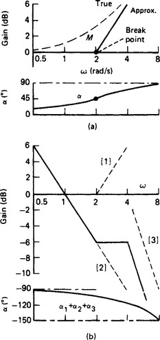
(3) 1 + j ωT: a straight line of zero gain for frequencies up to that for which ωT = 1, and thereafter a second straight line rising at 6dB per octave; the change of direction occurs at the break point (Figure 3.35(a)).
(4) 1/(1 + J ωT): as for 1 + J ωT, except that after the break point the gain drops with frequency at 6 dB per octave.
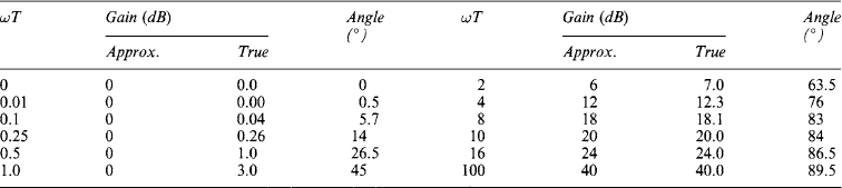
In Figure 3.35(a) the true gain shown by the broken curve is approximated by the two straight lines meeting at the break point. The approximate and true gains, and the phase angles, are given in Table 3.5 for the term 1 + J ωT. The error in the gain is 3 dB at the break point, and 1 dB at one-half and twice the break-point frequency, making correction very simple.
The uncorrected Bode plot for the system function
is shown in Figure 3.35(b). Term [1] is the same as in Figure 3.35(a). Term [2] is a straight line running downward through ω = 1 with a slope of 6 dB per octave. Term [3] has a break point at ω = 4, but as it is a squared term its slope for ω > 4 is 12 dB per octave. The full-time plot of gain is obtained by direct superposition. The effect of the constant K is to lift the whole plot upward by 20 log (K). The summed phase angles approach −90° at zero frequency and −180° at infinite frequency.
Nichols diagram The Nichols diagram resembles the Nyquist diagram in construction, but instead of phasor values the magnitudes are the log moduli. The point (-1 + j0) of the Nyquist diagram becomes the point (0 dB, ∠ − 180°). The Nichols diagram is used for determining the closed-loop response of systems.
3.2.16 Non-linearity
A truly linear system, in which effect is in all circumstances precisely proportional to cause, is a rarity in nature. Yet engineering analyses are most usually based on a linear assumption because it is mathematically much simplified, permits of superposition and can sometimes yield results near enough to reality to be useful. If, however, the non-linearity is a significant property (such as magnetic saturation) or is introduced deliberately for a required effect (as in rectification), a non-linear analysis is essential. Such analyses are mathematically cumbersome. No general method exists, so that ad hoc techniques have been applied to deal with specific forms of non-linearity. The treatment depends on whether a steady-state or a transient condition is to be evaluated.
3.2.16.1 Techniques
Some of the techniques used are: (i) step-by-step solution, graphical or by computation; (ii) linearising over finite intervals; (iii) fitting an explicit mathematical function to the non-linear characteristic; and (iv) expressing the nonlinear characteristic as a power series.
Step-by-step solution: Consider, as an example, the growth of the flux in a ferromagnetic-cored inductor in which the inductance L is a function of the current i in its N turns. Given the flux magnetomotive-force (m.m.f.) characteristic, and the (constant) resistance r, the conditions for the sudden application of a constant voltage V are given by
which is solved in suitable steps of Δt, successive currents i being evaluated for use with the magnetic characteristic to start the next time-interval.
Linearising: A non-linear characteristic may be approximated by a succession of straight lines, so that a piecemeal set of linear equations can be applied, ‘matching’ the conditions at each discontinuity.
For ‘small-signal’ perturbations about a fixed quiescent condition, the mean slope of the non-linear characteristic around the point is taken and the corresponding parameters derived therefrom. Oscillation about the quiescent point can then be handled as for a linear system.
Explicit function: For the resistance material in a surge diverter the voltage—current relationship v = kix has been employed, with x taking a value typically between 0.2 and 0.3. The resistance—temperature relationship of a thermistor, in terms of the resistance values R1 and R2 at corresponding absolute temperatures T1 and T2 takes the form
Several functions, such as y = a sinh (bx), have been used as approximations to magnetic saturation excluding hysteresis. A static-friction effect, of interest at zero speed in a control system, has been expressed as y = k(sgn x), i.e. a constant that acts against the driving torque.
Series: A typical form is y = a0 + a1 x + a2x2 + … + anxn, where the coefficients a are independent of x. Such a series may have a restricted range, and the powers limited to even orders if the required characteristic has the same shape for both negative and positive y. A second-degree series y = a0 + a1x + a2x2 can be fitted through any three points on a given function of y, and a third-degree expression through any four points. However, the prototype characteristic must not have any discontinuities.
Rational-fraction expressions have also been developed. The open-circuit voltage of a small synchronous machine in terms of the field current might take the form v = (27 + 0.006i)/(1 + 0.03i). Similarly, the magnetisation curve of an electrical sheet steel might have the B—H relationship
with hysteresis neglected. An exponential series
has been suggested to represent the magnetisation characteristic of a machine, the final term being related to the air gap line.
Non-linear characteristics Figure 3.36 shows some of the typical relations y = f(x) that may occur in non-linear systems. Not all are analytic, and some may require step-by-step methods.
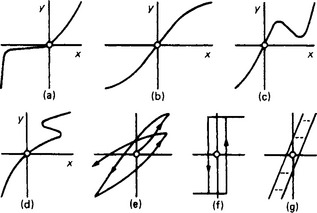
The simple relations shown are: (a) response depending on direction, as in rectification; (b) skew symmetry, showing the effect of saturation; and (c) negative-slope region, but with y univalued.
The complex relations are: (d) negative-slope region, with y multivalued; (e) build-up of system with hysteresis, unsaturated; (f) toggle characteristic, typical of idealised saturated hysteresis; and (g) backlash, with y taking any value between the characteristic limit-lines.
3.2.16.2 Examples
A few examples of non-linear parameters and techniques are given here to illustrate their very wide range of interest.
Resistors: Thermally sensitive resistors (thermistors) may have positive or negative resistance-temperature coefficients. The latter have a relation between resistance R and absolute temperature T given by R2 = R1 exp [b (1/T2 − 1/T1)]. They are made from oxides of the iron group of metals with the addition of small amounts of ions of different valency, and are applied to temperature measurement and control. Thermistors with a positive resistance-temperature coefficient made from monocrystalline barium titanate have a resistance that, for example, increases 100-fold over the range 50–100°C; they are used in the protection of machine windings against excessive temperature rise.
Voltage-sensitive resistors, made in disc form from silicon carbide, have a voltage—current relationship approximating to v = kiβ, where β ranges from 0.15 to 0.25. For β = 0.2 the power dissipated is proportional to v6, the current doubling for a 12% rise in voltage.
Inductors: The current in a load fed from a constant sinusoidal voltage supply can be varied over a wide range economically by use of a series inductor carrying an additional d.c.-excited winding to vary the saturation level and hence the effective inductance. The core material should have a flux-m.m.f. relationship like that in Figure 3.36(f). Grain-oriented nickel and silicon irons are suitable for the inductor core. A related phenomenon accounts for the in-rush current in transformers.
Describing function: In a non-linear system a sinusoidal drive does not produce a sinusoidal response. The describing-function technique is devised to obtain the fundamental-frequency effect of non-linearity under steady-state (but not transient) conditions.
Consider a stimulus x = h cos ωt to give a response y = f(t). As non-linearity inevitably introduces harmonic distortion, y can be expanded as a Fourier series (Section 1.2.5) to give
The components a1 cos ωt and b1 sin ωt are regarded as the ‘true’ response, with a gain factor (a1 + jb1)/h, the other terms being the distortion. The gain factor is the describing function. Let y = ax + bx2 with x = h cos ωt; applying the expansion gives the fundamental-frequency term ![]() . The describing function is therefore
. The describing function is therefore ![]() , which is clearly dependent on the magnitude h of the input. Thus the technique consists in evaluating the Fourier series for the output waveform for a sinusoidal input, and finding therefrom the magnitude and phase angle of the fundamental-frequency response.
, which is clearly dependent on the magnitude h of the input. Thus the technique consists in evaluating the Fourier series for the output waveform for a sinusoidal input, and finding therefrom the magnitude and phase angle of the fundamental-frequency response.
Ferroresonance: The individual r.m.s. current—voltage characteristics of a pure capacitor C and a ferromagnetic-cored (but loss-free) inductor L for a constant-frequency sinusoidal r.m.s. voltage V are shown in Figure 3.37. With L and C in series and carrying a common r.m.s. current I, the applied voltage is V = VL−VC. At low voltage VL predominates, and the I−V relationship is the line 0P, with I lagging V by 90°. At P, with V = V0 and I = I0, the system is at a limit of stability, for an increase in V results in a reduction in VL−VC. At a current level Q the difference is zero. The current therefore ‘jumps’ from I0 to a higher level I1 (point R), still with V = V0. During the rapid rise there is an interchange of stored energy, and for V > V0 the circuit is capacitive. When V is reduced from above to below V0, a sudden current jump from I1 to I0 occurs. A comparable jump phenomenon takes place for a parallel connection of C and L.
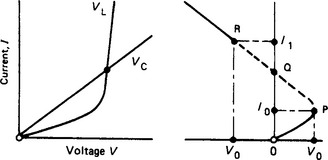
Phase-plane technique: ‘Phase’ here means ‘state’ (as in the solid, liquid and vapour ‘phases’ of water). The phase-plane technique can be used to elucidate non-linear system behaviour graphically. Figure 3.38 shows a circuit of series R, L and C with a drive having the voltage—current relationship v = −ri + ai3. Then, with constant circuit parameters,
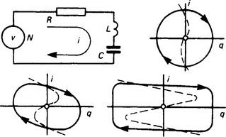
where q is the time-integral of i. The presence of L and C indicates the possibility of oscillation. The middle (‘damping’) term can be negative for small currents (increasing the oscillation amplitude) but positive for larger currents (reducing the amplitude). Hence the system seeks a constant amplitude irrespective of the starting condition. The q − i phase-plane loci show the stable condition as related to the degree of drive non-linearity (indicated by the broken curves). With suitable scales the locus for minor non-linearity is circular, indicating near-sinusoidal oscillation; for major drive non-linearity, however, the locus shows abrupt changes and an approach to a ‘relaxation’ type of waveform.
Isoclines: A non-linear second-order system described by
can be represented at any point in the phase plane having the co-ordinates y and dy/dt, representing, for example, position and velocity, or charge and current. By writing dy/dt = z and eliminating time by division, we obtain a first-order equation relating z and y:
Integration gives phase-plane trajectories that everywhere satisfy this equation, starting from any initial condition. If dz/dy cannot be directly integrated, it is possible to draw the trajectories with the aid of isoclines, i.e. lines along which the slope of the trajectory is constant. Make dz/dy = m, a constant; then −mz = f(y, z)z + g(y, z)y. Since for z = 0 the slope m is infinite (i.e. at right angles to the y axis) the trajectories intersect the horizontal y axis normally, except at singular points.
Consider a linear system with an undamped natural frequency ωn = 1 and a damping coefficient c = 0.5. For zero drive
if z is written for dy/dt. Dividing the second equation by z and equating it to a constant m gives
representing a family of straight lines with the associated values
Draw the z/y axes on the phase plane (Figure 3.39) marked with short lines of the appropriate slope m. Then, starting at any arbitrary point, a trajectory is drawn to cross each axis at the indicated slope. With no drive, all trajectories approach, and finally reach, the origin after oscillations in a counter-clockwise direction; for a steady drive V, the only difference is to shift the vortex to V on the j-axis. The approach to O or V represents the decaying oscillation of the system and its final steady state. Because dt = dy/z, the finite difference Δt = Δy/z gives the time interval between successive points on a trajectory.
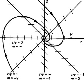
3.3 Power-system network analysis
Modern power-system analyses are based mainly on nodal equations scaled to a per-unit basis, with a particular convention for the sign of reactive power.
3.3.1.1 Per-unit basis
The total apparent power in a three-phase circuit ABC with phase voltages Va, Vb, Vc, currents Ia, Ib, Ic and phase angles between the associated voltage and current phasors of θa, θb, θc is
where for phase A the active power is Pa = VaIa cos θa and the reactive power is Qa = VaIa sin θa. Corresponding expressions apply for phases B and C.
If the phases are balanced, all three have the same scalar voltage V and current I, and all phase angles are θ. Then S = 3(VI cos θ + jVI sin θ). This can be written in the form
where k, a, b, c and d are scaling factors. It is customary to choose a = 3 and d = 1, leaving c and b, one of which is assigned an independent value while the other takes a value depending on the overall scaling relation k = abcd.
In normal operating conditions the scalar voltage V approximates to the rated phase voltage VR; hence b is taken as VR so that V/b is the voltage in per unit of VR. Defining the scaled variables as Spu, Vpu and Ipu, the total apparent power is
which is an equation in one-phase form, justifying the use of single-line schematic diagrams to represent three-phase power circuits.
The scaling factors are termed base values; i.e. k is the base apparent power, b is the base phase voltage and c is the base current. These definitions imply further base values for impedance and admittance, namely Zbase = b/c and Ybase = c/b.
If the line-to-line voltage Vt is used, then in the foregoing scaling equation 3/a and V/b becomes ![]() and Vt/b′. Choosing
and Vt/b′. Choosing ![]() and b′ as rated line voltage leaves S/k unchanged. Note, however that: (i) θ remains as the angle between phase voltage and current; and (ii) in the per-unit equation S = VI* the voltage V is the per-unit phase voltage, not the line-to-line voltage (although numerically both have the same per-unit value).
and b′ as rated line voltage leaves S/k unchanged. Note, however that: (i) θ remains as the angle between phase voltage and current; and (ii) in the per-unit equation S = VI* the voltage V is the per-unit phase voltage, not the line-to-line voltage (although numerically both have the same per-unit value).
3.3.1.2 Reactive power convention
Reactive power may be lagging or leading. The common convention is to consider lagging reactive power flow to be positive, as calculated from the product of the voltage and current-conjugate phasors: thus S = VI* = P + jQ, with Q a positive number for a lagging power factor condition. For a leading power factor, Q has the same flow direction but is numerically negative. As a consequence, an inductor absorbs, but a capacitor generates, lagging reactive power, as shown in Figure 3.40.
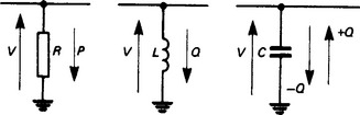
Note: system engineers refer, for brevity, to the flow of ‘power’ and ‘vars’, meaning active power and reactive power, respectively.
3.3.1.3 Nodal-admittance equations
The nodal-admittance equations derive from the node-voltage method of analysis in Section 3.2.3. For the network in Figure 3.41, currents I1, I2 and I3 are injected respectively into nodes 1, 2 and 3. The loads are linked by branches of admittance y12, y23 and y31, and to the earth or external reference node r by branches of admittance y10 and y30. Assuming that the node voltages V1, V2 and V3 are expressed with reference to r and that Vr = 0, then writing the Kirchhoff current equations and simplifying gives
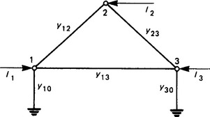
Cast into matrix form, these equations become
This can be abbreviated to the nodal-admittance matrix equation YV = I, matrix Y being known as the nodal-admittance matrix. The relationship between the branch elements and the corresponding matrix elements can be seen by inspection.
For some purposes the alternative impedance matrix equations are used: viz. ZI = V, where Z = Y−1 is the nodal-impedance matrix. However, evaluating the inverse of Y is more complicated than finding Y, and the admittance form may be considered as the primary (or given) form.
3.3.2 Load-flow analysis
Load-flow analysis is the solution of the nodal equations, subject to various constraints, to establish the node voltages. At the same time generator power outputs, transformer tap settings, branch power flows and powers taken by voltage-sensitive loads (including reactive power compensators) are determined.
3.3.2.1 Problem description
As indicated in Figure 3.41, the elements of a power system can be represented either as equivalent branches with appropriate admittance incorporated into the matrix Y, or as equivalent current sources added to the matrix I.
Transmission lines and cables: These are represented by their series admittance and shunt (charging) susceptance. These parameters are actually distributed quantities, but are taken into account by II (or, occasionally, T) equivalent networks (Section 3.2.5).
Transformers: These are modelled by equivalent circuits with an ideal transformer in series with a leakage admittance (Figure 3.42(a)). With two terminals connected to a common reference point (earth) the circuit reduces to that in Figure 3.42(b): the ideal transformer with a turns ratio (1 + t)/1 is replaced by an equivalent II. The tap setting t represents the per-unit of nominal turns ratio: e.g. t = ±0.05 for ±5% taps.
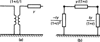
Loads: These can be represented either as equivalent admittances Yk0 connected between bus-bars and earth, or as current sources. If the load demand at bus-bar k is Sk = Pk + jQk, then the equivalent admittance at voltage Vk is found from
where |Vk| is assumed to be 1.0 p.u. (i.e. rated voltage). The equivalent admittance is incorporated into the corresponding diagonal element of the nodal-admittance matrix. In the current-source representation, the current Ik is substituted into the current column-matrix I by a fixed power requirement Sk and the (unknown) voltage Vk, where ![]() .
.
Generator units or stations can likewise be represented by current sources, but usually the bus-bar to which a generator is connected has a controlled voltage. At a bus-bar m the requirement would be for specified values of active power Pm and voltage |Vm|, with the reactive power Qm to be determined.
Slack bus-bar: In a load-flow study, the total active power supplied cannot be specified in advance because the loss in the supply network will not be known. Further, in an n-bus-bar network, there are n complexor equations involving 2n real-number equations. However, there are 2n + 2 unknowns. To reduce this number to 2n it is the practice to specify the voltage of one bus-bar in both magnitude and phase angle. This is termed the slack bus-bar, to which the chosen slack generator is connected. The slack-bus-bar equation can now be removed from the solution process and, when all other voltages have been determined, the slack-bus-bar generation can be found. For a slack bus-bar k, for example, the generation Sk is found from
3.3.2.2 Network solution process
Solution of the matrix equation is now sought. As it embodies several simultaneous equations, the solution has to be iterative. The two main procedures are the Gauss—Seidel and the Newton—Raphson methods. An important consideration in the computation process is the rate of convergence.
3.3.2.3 Gauss—Seidel procedure
This early (and still effective) technique resembles the over-relaxation method used in linear algebra. Consider a four bus-bar network described by the equations
where Y12 = −y12, etc. Let bus-bar 1 be chosen as the slack bus-bar, and let V1 be 1 + j0. Then the remaining three equations are to be solved for V2, V3 and V4. The method adopted is one of successive estimation.
First, the equations are rearranged by extracting the diagonal terms Y11 V1, Y22 V2, …, and transferring all other terms to the right-hand side. Each equation is then divided by the diagonal admittance element (Y11, Y22, …).
If ![]() denotes the p th estimate of Vk and the equations are solved in the sequence 2–3–4–2–3- …, then an iterative process is the following:
denotes the p th estimate of Vk and the equations are solved in the sequence 2–3–4–2–3- …, then an iterative process is the following:
Note that as each new estimate becomes available, it is used in the succeeding equations. Being iterative, the process of convergence can usually be assisted by the use of ‘acceleration’. If ![]() , then a new estimate can be obtained from
, then a new estimate can be obtained from ![]() here ω is an accelerating factor, optimally a complex number but usually taken as real, with typical values in the range 1.0–1.6.
here ω is an accelerating factor, optimally a complex number but usually taken as real, with typical values in the range 1.0–1.6.
To terminate the successive-estimation process, various convergence tests are applied. The simplest is to examine the difference between successive voltage estimates and to stop when the maximum of ![]() for k = 1, 2,…, n is less than ε, a suitable small number such as 0.000 01 p.u. However, the preferred test is
for k = 1, 2,…, n is less than ε, a suitable small number such as 0.000 01 p.u. However, the preferred test is
where γ is a measure of the maximum allowable apparent-power mismatch at any bus-bar, with a value typically 0.01 p.u.
During iteration, other calculations (e.g. voltage magnitude corrections at generator bus-bars and changes in transformer tap settings) can be included. If bus-bar 2 in the example above is a generator bus-bar, then the reactive power Q2 can be assigned an initial value, say Q2(0) = 0, and V2(1) obtained therefrom. The voltage estimate can then be scaled to agree with the specified magnitude |V2|, and Q2(1) immediately calculated, prior to proceeding to the next equation.
The Gauss—Seidel procedure is well suited to implementation on a microcomputer, in which core space is limited. However, matrix-inversion techniques (as required in the Newton—Raphson procedure following) for large networks demand too much core space.
3.3.2.4 Newton—Raphson procedure
The Newton—Raphson procedure is at present the most generally adopted method. It has strong convergence characteristics and suits a wide range of problems. The method employs the preliminary terms in the Taylor series expansion (Section 1.2.4) of a set of functions of variables V. The k th function is defined as
The true set of values V is taken as given by V = V(p) + γ(p), i.e. by the sum of an approximate set V(p) and a set of error terms γ(p). Then, taking the first two terms of the Taylor expansion,
Matrix J(V(p)) is the Jacobian matrix of first derivatives of the functions f(V). Voltage estimates V(p) are used to evaluate specific matrix elements of J; and γ(p) is the column matrix of voltage differences ΔV(p) to be evaluated, these being the difference between the true and approximate values of the voltages V. Likewise, the term -f(V(p)) is the set of per-unit apparent-power differences ΔS(p) between specified and calculated values, where
The load-flow equation to be solved becomes
When ΔV(p) is determined, the voltages are updated to V(p + 1) = V(p) + ΔV(p).
The polar form of the equations is most usually employed, so with Vk = |Vk| ∠δk and Ykm= |Ykm|∠ ψkm the function fi = 0 becomes
where βi1 = δi − δ1 − ψi1 and similarly for βi2, … Partial differentiation to form the terms of the Jacobian matrix, and then separation of the real and imaginary parts, gives the matrix equations to be solved. For generator bus-bars the voltage magnitudes are fixed, so that only equations in reals are needed to evaluate ∠ δ.
Generator bus-bars are often termed ‘P, V’ and load bus-bars referred to as ‘P, Q’ bus-bars, reflecting the values specified.
The Jacobian equations for the Newton—Raphson method are thus of the form
Written in abbreviated form, this is
To save computer-memory space, it is usual to omit J12 and J12, an approximation that leaves two decoupled sets of equations. This approach, called the ‘fast decoupled Newton—Raphson loadflow’, is in wide use.
For any set of estimates of the voltage, the elements of the Jacobian matrix are evaluated, and the set of equations solved (using space-saving sparse-matrix programming techniques) for Δδ and ΔV; the values of V, ΔP and ΔQ are updated, and so on. Convergence is achieved for most networks in a few iterations.
A further development is to extend the Taylor series to the second-derivative term, when the series will terminate if Cartesian co-ordinates are employed. Iteration is more lengthy, but the convergence characteristics are more powerful. This ‘second-order Newton—Raphson procedure’ is gaining popularity.
3.3.3 Fault-level analysis
The calculation of three-phase fault levels in large power networks again involves solution of the nodal-admittance equations YV = I subject to constraints.
3.3.3.1 System representation
Representation of generators and loads by fixed P, |V| and P, Q requirements is not valid because of the large and sudden departure of the bus-bar voltages from their nominal values.
Passive loads are usually represented by a constant admittance, implying that the load power is proportional to the square of the bus-bar voltage. Relations P α |V|1.2 and Q α |V|1.6 would be more likely, but the |V|2 proportionality affords a measure of demand variability and is more easily represented in the admittance matrix Y.
Synchronous machines such as generators and motors are represented by a voltage source in series with an appropriate admittance. For example, at bus-bar k where the node voltage is Vk, the current could be represented by ![]() using the subtransient e.m.f. and admittance. The term
using the subtransient e.m.f. and admittance. The term ![]() can be transferred to the other side of the nodal-admittance equation in such a way that yk″ joins any load-admittance term in the diagonal element Ykk.
can be transferred to the other side of the nodal-admittance equation in such a way that yk″ joins any load-admittance term in the diagonal element Ykk.
The network equations have now been modified to the form
where Y″ is the admittance matrix Y with diagonal elements supplemented by equivalent load admittances and machine subtransient admittances, and the right-hand-side elements are either of the type ![]() or zero.
or zero.
3.3.3.2 Method of solution
In three-phase short-circuit conditions the voltages V will differ from the steady-state load values, but the right-hand-side elements will, with the exception of the element corresponding to the faulted bus-bar, remain constant. Let bus-bar m be short circuited; then Vm = 0. Solving the remaining equations for the voltages Vi (with i = 1, 2, …, n, i ≠ m) by the Gauss—Seidel procedure and then substituting the voltage values obtained in the m th equation yields a new right-hand-side value of one or other of the forms
Here Imsc is the three-phase per-unit short-circuit current injected into bus-bar m to make Vm = 0. The fault level (in megavolt-amperes (MV-A)) is then
A preferred alternative uses the superposition theorem (Section 3.2.2.1). The injection of Imsc, when acting alone, superposes a change ΔVm (= −Vm(prefault)) at bus-bar m. The equations to be solved become
Inversion of Y″ gives V = Z″ Isc, in which the m th equation is known to be −Vm = Zmm″ Im sc. If we assume nominal prefault voltage, i.e. Vm = 1 + j0 p.u., then the value of the three-phase short-circuit current at bus-bar m is Im sc = −1/Zmm″. The voltage at any other bus-bar k can then be found from
By shifting the short circuit from bus-bar to bus-bar, the fault level for each can be found from the inverses of the appropriate diagonal elements of matrix Z″.
3.3.4 System-fault analysis
The analysis of unbalanced faults in three-phase power networks is an important application of the symmetrical-component method (Section 3.2.12). The procedure for given fault conditions is as follows.
(1) Obtain the sequence impedance values for all items of the plant, equipment and transmission links concerned.
(2) Reduce all ohmic impedances to a common line-to-neutral base and a common voltage.
(3) Draw a single-line connection diagram for each of the sequence components, simplifying where possible (e.g. by star—delta conversion, see Section 3.2.4.5).
(4) Calculate the z.p.s., p.p.s. and n.p.s. currents, tracing them through the network to obtain their distribution with reference to the particular values sought.
Impedance in the neutral connection to earth, and in the earth path itself, must be multiplied by 3 for z.p.s. currents when the z.p.s. connection diagram is being set up in (3) because the three z.p.s. component currents are co-phasal and flow together in the z.p.s. path.
In general, a network offers differing impedances Z+, Z− and Z0 to the sequence components. In static plant (e.g. transformers and transmission lines) Z− may be the same as Z+, but Z0 is always significantly different from either of the other impedances. The presence of z.p.s. currents implies that a neutral connection is involved.
3.3.4.1 Sequence networks
As an example, Figure 3.43 shows transmission lines 4 and 5–6 linking a generating station with generators 1 (isolated neutral) and 2 (solid-earthed neutral) to a second station with generator 3 (neutral earthed through resistor Rn). The numerals are used to indicate position: e.g. Z1+ is the p.p.s. impedance per phase of generator 1, and Z60 is the z.p.s. impedance of line 6 between generator 3 and a fault at F.
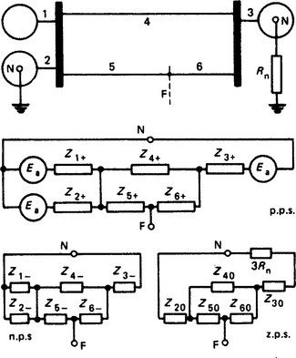
The p.p.s. network is identical with the physical set-up of the original network (which operates with p.p.s. conditions when normally balanced and unfaulted). Each generator is a source of p.p.s. voltages only. It is here assumed that all the generators develop the same e.m.f. Ea.
The n.p.s. network is similar in configuration (but not usually in impedance values) to the p.p.s. system. There are, however, no source e.m.f.s: the n.p.s. voltages are ‘fictitious’ ones developed by the fault.
The z.p.s. network is radically different from the other two, being concerned with neutral connections and earth faults. The effective line impedance is that of three conductors sharing equally the total n.p.s. current. To this must be added the earth-connection and earth-path impedances multiplied by 3, to give the z.p.s. impedance Z0.
Typical values of Z− and Z0 in terms of Z+ are
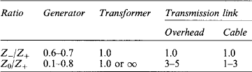
The value of Z0 for a synchronous generator depends on the arrangement of the stator winding.
To evaluate the system when faulted, it is necessary to determine the fault currents and the voltage of the sound line(s) to earth. If the voltages and currents at the fault are Va, Vb, Vc and Ia, Ib, Ic, respectively, the following expressions always apply:
where α is the 120° rotation operator (see Section 3.2.12). From the boundary conditions at the fault concerned it is possible to write three equations and to solve them for the symmetrical components I+, I− and I0.
Sequence networks for some of the many transformer connections are shown in Figure 3.44. Further sequence networks are given in reference 1.
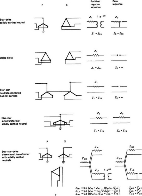
3.3.4.2 Boundary conditions
Three simple cases are shown in Figure 3.45. It is assumed that only fault currents are concerned, and that in-feed to the fault is from one direction.
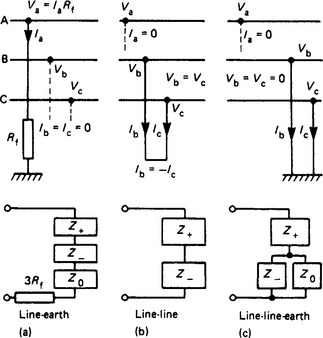
(a) Earth fault of resistance Rf on line A—at the fault, Va = IaRf and Ib = Ic = 0. This leads to Ia0 = Ia+ = Ia-, so that the three sequence currents in phase A are identical. It follows that Ib and Ic are zero, as required. From the basic equations
and the fault current is Ia = 3Ea/Z. The three sequence networks are, in effect, connected in series. The component currents, and the voltages Vb and Vc, are obtained from those in phase A by application of the basic relations in Section 3.3.4.1. Each sequence current divides in the branches of its network in accordance with the configuration and impedance values.
(b) Short circuit between lines B and C—the boundary conditions are Ia = 0, Ib = −Ic and Vb = Vc. As there is no connection to earth at the fault, the z.p.s. network is omitted. The p.p.s. and fault currents are
where Z = Z+ + Z− is the impedance of the p.p.s. and n.p.s. networks in series. The voltages to neutral at the fault are
(c) Double line-earth fault on lines B and C—here the boundary conditions are Ia = 0, and Vb = Vc = 0. The sequence components of the fault current are
The sequence networks are connected in series-parallel.
Figure 3.46 shows the interlinked phase-sequence networks where both ends feed the fault F. Conditions in (a), (b) and (c) correspond to those in Figure 3.45. Networks for a broken-conductor condition are shown in (d) and (e): the former is for a case in which both ends at the break remain insulated, while the latter applies where the conductor on side 2 falls to earth, the additional constraint involving ideal 1/1 transformers in side 2 of the combined sequence network. In more complicated cases, ideal transformers with phase-shift or with ratios other than 1/1 may be required. Evaluation of these, and of conditions involving simultaneous faults at different points and/or phases, requires matrix analysis and computer programs.
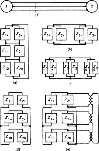
3.3.5 Phase co-ordinate analysis
The same techniques developed for the analysis of balanced networks, i.e. load-flow and three-phase fault-level analysis, can be used to develop the analysis of unbalanced faults or loads on either balanced or unbalanced networks using a phase representation of the system. The symmetrical component theory, which has formed the basis of unbalanced power system network analysis, was developed by several authors between 1912 and 1918. Although forming the basis of most modern computer-aided fault analyses, the method is limited by both balanced network assumptions and the difficulties associated with finding equivalent network models in the space described by the set of (transformed) 0, 1, 2 variables, e.g. for simultaneous faults.
The phase co-ordinate method described here uses only the primary phase a, b, c variables and computer-based matrix computational methods to solve the resulting equations subject to the necessary constraints imposed by load-flow or fault analyses.2–6
3.3.5.1 Element representation
For brevity, when referring to the sequence frame of reference, only the zero-, positive- and negative-sequence components usually associated with Fortescue will be discussed.
General element: The general network element of the power system shown in Figure 3.47 for a three-phase system may be described in matrix form by
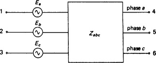
where Vabc represents the per-phase series voltage drops (V1 − V4), (V2 − V5) and (V3 − V6), Eabc is the matrix of the equivalent voltage sources per phase, Iabc is the matrix of currents flowing per phase between nodes 1 and 4, 2 and 5, and 3 and 6, respectively, and Zabc represents the passive three-phase mutually coupled network.
Defining the transformation relating the phase to the sequence components by
where α = 1 ∠ 120° and, for the usual Fortescue components V0, V1 and V2, will be used instead of the rather cumbersome notation V0, V+ and V−; thus
Noting that ![]() , upon transformation the equivalent sequence relationship becomes
, upon transformation the equivalent sequence relationship becomes
For the customary linear device Zabc is symmetric, but without further assumptions Z012 is unsymmetric.
Transmission lines: The series relationships along a transmission line may be represented by the partitioned equations
where V1 and V2 are column submatrices representing the series voltages along conductors and subconductors, respectively, carrying the currents in the submatrices I1 and I2. I3 is a submatrix representing the currents in any earth wires present, which are assumed to be solidly earthed at each end. This latter assumption is normal, but unnecessary, for the solution of the system equations, because extra equations representing earth wires can be included for solution.
A matrix reduction (completion of bundling process and earth-wire removal) will then yield the equations of the equivalent phase conductors, thus giving
The 3 × 3 matrix Zabc represents the series impedance of the transmission line, including all the effects due to unbalanced configuration and the use of bundled conductors and earth wires. In a three-phase representation of the network this matrix may be treated in the same way as the single series impedance of the more usual one-line diagram.
By similar reasoning, the potential coefficients of the transmission line (phase and earth wires) per unit of length may be computed for any configuration. From these coefficients a shunt-reactance matrix is found, and then, by reduction, the 3 × 3 matrix Zshunt representing the total distributed capacitive reactance over the length of the line. Inverting this matrix gives Yshunt from which the Maxwell coefficients, and hence capacitances, can be determined if necessary.
Three-phase transmission-line models follow as extensions of the nominal or distributed π and T representations. In the π representation one-half of the transmission-line equivalent capacitance is connected to each end of the line.
The nodal voltages and currents injected into the busbars at each end of the transmission line are then related by
The similarity between the three-phase and single-phase admittance matrices is evident—each element in the single-phase matrix is replaced by the appropriate 3 × 3 admittance sub-matrix.
Machine representation: The general element shown in Figure 3.47 may be taken to represent any synchronous or induction machine with a star-connected stator winding when nodes 1, 2 and 3 are short circuited. For a balanced design the voltage sources would be displaced 120° from each other and be equal in magnitude.
The phase-impedance matrix Zabc can be found by simple transformation of the normally available sequence impedance matrix, as indicated in equations (3.3) and (3.4). The sequence impedance matrix here reflects the structure of the machine and the purpose of the study in the selection of the positive sequence reactance. A typical salient-pole diesel generator, for example, with segmented dampers, 14 poles and 90.7% winding pitch rated at 1340 kV-A, 3.3 kV, 50 Hz has negative and zero reactances of X2 = 0.274 p.u. and X0 = 0.067 p.u., respectively. In a fault-level study the machine is represented in the positive-sequence circuit by the subtransient reactance X′d = 0.227 p.u. = X1. The phase-impedance matrix would then be
Note that, with X1 ≠ X2, the phase-impedance matrix elements contain both positive and negative real parts, although no resistances were included in the sequence impedances.
Such a representation neglects the effective winding capacitances. These capacitances could be added, if necessary, in the same manner as the transmission-line capacitances in the three-phase representation in delta and shunt connections (a four-terminal lattice network with one terminal earthed). Neglected also is any representation of a machine neutral node. Instead of adding an appropriate row or column to Zabc, the effect of any earthing reactance Xg can be included in the value of X0, i.e. X0 + 3Xg.
Transformer representation: The third type of network element is the transformer in one-, two- and three-phase circuits with all the associated possible variations of construction and connection.
(a) Derivation of equivalent-circuit model: A single-phase representation of a transformer in per-unit form illustrated schematically in Figure 3.48 by an ideal transformer of turns ratio (1 + t):1 with an equivalent leakage admittance of y per unit.
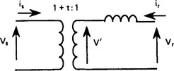
From the relationships across the ideal transformer an equivalent circuit model is as shown in Figure 3.49 and thus represents a single-phase tapped transformer.
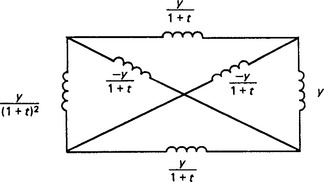
Figure 3.49 Symmetrical lattice equivalent circuit of a single-phase transformer with a variable turns ratio
If nodes k and q are earthed as in the one-line diagram representation of a balanced three-phase system, the lattice circuit reduces to the equivalent π representation, as shown in Figure 3.50.
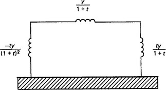
The lattice equivalent of Figure 3.49 provides an adequate model for single-phase variable-turns-ratio transformers and in combinations for three-phase star-star banks with tapped windings, but can only be used with care in banks containing delta-connected windings. In a star—delta bank of single-phase transformer units, for example, with normal turns ratio, a value of 1.0 p.u. voltage on each leg of the star winding produces under balanced conditions 1.732 p.u. voltage on each leg of the delta winding (rated line to neutral voltage as base). The structure of the bank requires in the per-unit representation an effective tapping at ![]() times nominal turns ratio on the delta side, i.e. 1 + t = 1.732 or t = 0.732.
times nominal turns ratio on the delta side, i.e. 1 + t = 1.732 or t = 0.732.
For a delta—delta or star—delta transformer with taps on the star winding, the equivalent circuit of Figure 3.49 would have to be modified to allow for effective taps to be represented on each side. This, the general symmetrical lattice equivalent circuit of a single-phase transformer where both primary and secondary windings may have either actual or equivalent variable turns ratios α and β or both is shown in Figure 3.51. This single-phase transformer model can be used to assemble equivalent circuits of polyphase transformer banks, some of which are shown below
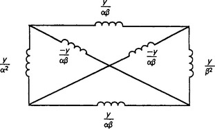
(b) Star-star transformer: For a two-circuit three-phase transformer or autotransformer connected in a star-star arrangement, the equivalent circuit is as shown in linear-graph form in Figure 3.52. Parallel transformer windings are taken to represent equivalent single-phase transformers. The circuit is constructed from the simple connection of three of the general circuits shown in Figure 3.51 with taps on both windings. In practice, of course, either α or β, or both, would be 1.0 p.u.
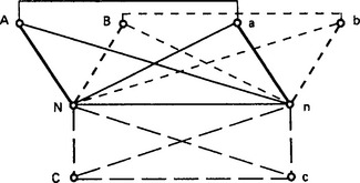
In a more concise form, the equivalent circuit of Figure 3.52 may be described by the connection table given in Table 3.6 where, for example, an admittance of value y/α2 is connected between N and A, also N and B, etc. If the neutrals are earthed or connected together either solidly or through an impedance, the appropriate additions or deletions can be made to the circuit and corresponding terms changed in the connection table. From inspection of the circuit, the corresponding admittance matrix can be assembled with or without rows and columns for the neutral nodes, depending on the earthing arrangements.
Table 3.6
Connection table for the star—star transformer equivalent circuit shown in Figure 3.52 (α = 1 + tα p.u.; β = 1 + tβ p.u.)
| Admittance | Between nodes |
| y/α2 | N—A, N—B, N—C |
| y/β2 | n—a, n—b, n—c |
| y/αβ | A—a, B—b, C—c |
| −y/αβ | n—A, n—B, n—C; N—a, N—b, N—c |
| 3y/αβ | N—n |
(c) Delta-delta transformer: With the same convention (that parallel windings may be considered to represent single-phase transformers) the equivalent circuit of a delta-delta transformer may be constructed by the same principles, as shown in Figure 3.53. The corresponding connection table is shown in Table 3.7, where both windings have variable ratios. With taps on one winding only either α or β would have the value ![]() , the tap value tα or tβ being zero accordingly.
, the tap value tα or tβ being zero accordingly.
Table 3.7
Connection table for the delta—delta transformer in the equivalent circuit shown in Figure 3.53 (![]() ;
; ![]() )
)
| Admittance | Between nodes |
| y/α2 | A—B, B—C, C—A |
| y/β2 | a—b, b—c, c—a |
| 2y/αβ | A—A, B—b, C—c |
| −y/αβ | A—b, B—c, C—a; a—B, b—C, c—A |
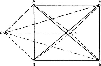
(d) Star—delta transformer: Using the same techniques, the three-phase equivalent circuit model of a star—delta transformer may be assembled and is shown in Figure 3.54. The convention used for numbering nodes and thus identifying opposite sides of the symmetrical lattice networks is as follows:
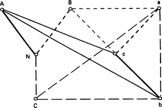
The connection table for Figure 3.54 is given in Table 3.8. Again, for taps on one side of the transformer only, either tα or tβ is zero. The neutral node N in the table can be identified with the reference earth node if solidly earthed or extra terms can be added to the table or not, according to the earthing arrangements
Table 3.8
Connection table for the star—delta transformer in the equivalent circuit shown in Figure 3.54 (α = 1 + tα p.u.; ![]() )
)
| Admittance | Between nodes |
| y/α2 | A—N, B—N, C—N |
| y/β2 | a—b, b—c, c—a |
| y/αβ | A—c, B—a, C—b |
| y/αβ | A—b, B—c, C—a |
(e) Three-winding transformers: With the same assumptions the analysis can be extended to three-circuit transformers and autotransformers and to any multiwinding transformer regardless of the number of circuits. Consider, for example, a star—star—delta transformer with solidly earthed neutrals. Let the star primary and secondary winding (P and S) terminals be labelled A, B, C, N and A′ B′, C′, N′, respectively, with the delta tertiary winding (T) terminals labelled a, b, c, as shown in Figure 3.55.
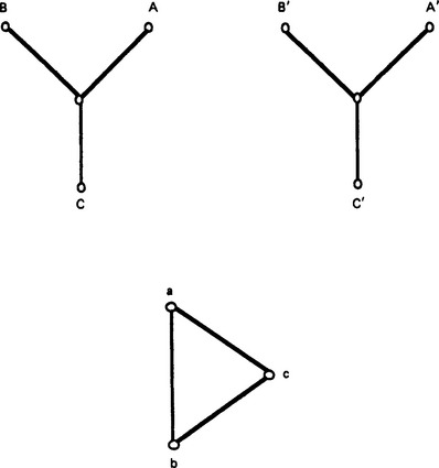
If yPS, yPT and yST are the short-circuit per-unit admittances of the two windings indicated by the subscripts with the third winding open, a three-phase equivalent circuit can be assembled from paralleling one star—star and two star—delta equivalent circuits in turn. The circuit line diagram is too complex to illustrate conveniently, but with the same convention concerning the matching of parallel sides in the identification of the single-phase units, A—N with A′—N′, A—N with c—b and A′—N′ with c—b, etc., the connection table will be as in Table 3.9, where α represents the turns ratio of winding P, β of winding S, and γ of winding T. Neutrals N and N′ are solidly earthed.
Table 3.9
Connection table for a three-winding star—star—delta transformer (α = 1 + tp p.u.; β = 1 + ts p.u.; ![]() )
)
| Admittance | Between nodes |
| (yPS + yPT)/α2 | N—A, N—B, N—C |
| (yPS + yST)/β2 | N′—A′, N′—B′, N′—C |
| yPS/αβ | A—A′, B—B′, C—C′ |
| −yPS/αβ | N′—A, N′—B, N′—C; N—A′, N—B′, |
| (yPT + yST)/±2 | N—C′ |
| yPT/αγ | a—b, b—c, c—a |
| yST/βγ | A—c, B—a, C—b |
| −yPT/αγ | A′—c, B′—a, C′—b |
| −yST/βγ | A—b, B—c, C—a |
| A′—b, B′—c, C′—a |
Note that, because two symmetrical lattice networks are connected to any two nodes on the same winding, a and b for example, the total admittance between these nodes is the sum of the corresponding admittances belonging to each of the two lattices between these nodes, e.g.
(f) Open-delta transformer: The validity of the equivalent-network model in representing unbalanced transformer designs is demonstrated in the analysis of the open-delta transformer. Figure 3.56 shows a schematic circuit diagram of the transformer with each delta open opposite nodes A and a, respectively. Connecting parallel branches of the windings by symmetrical-lattice equivalent circuits yields the connection table shown in Table 3.10.
Table 3.10
Connection table for the open—delta transformer with each winding open opposite nodes A and a respectively (![]() )
)
| Admittance | Between nodes |
| y/α2 | A—B, C—A |
| y/β2 | a—b, c—a |
| y/αβ | B—b, C—c |
| −y/αβ | A—b, A—c, B—a, C—a |
| 2y/αβ | A—a |
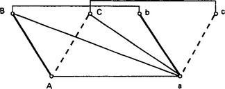
Equivalent circuits for other unbalanced transformers and for transformers with different numbers of primary and secondary phases, i.e. m-to-n transformers such as Scott, Zig-zag, Vee transformers, etc., can be found in reference 5.
Effects of magnetising impedances: The preceding transformer models do not account for the effects of core structure and saturation. In particular, it is noted that the phase circuits give the same representation as transformer sequence impedance circuits with a series impedance of equal value in each of the positive-, negative-, and zero-sequence circuits. More accurate representations include the transformer magnetising impedances in three-phase transformers.
In terms of the sequence quantities, these impedances are of particular importance in the zero-sequence networks. High values of zero-sequence voltage in shell-type transformers, and the effects of the tank walls and out-of-core return paths for zero-sequence fluxes in three-legged core-type transformers, give magnetising impedances of the same order of magnitude as the system impedances.
The transformer equivalent sequence networks can be modified to become T networks, with the magnetising impedance sequence components in the legs of the Ts. In phase coordinates the shunt impedance branch can be added likewise to the transformer single-phase model, as indicated in Figure 3.57. The dotted line indicates the part of the transformer short-circuit impedance placed in the lattice networks; the other part could be incorporated into a lattice network if equivalent taps are required on both sides. The equality of the series admittances has no significance.
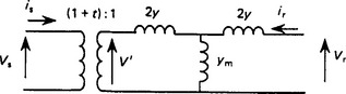
Figure 3.57 Per-unit schematic representation of a single-phase transformer with core representation
Starting from the usual measures of these magnetising admittances in sequence terms, the three-phase equivalent circuit can be developed as follows where, for a balanced design,
This phase-admittance matrix represents an equivalent delta network with connections to earth at each node where y1 = y2 as shown in Figure 3.58.
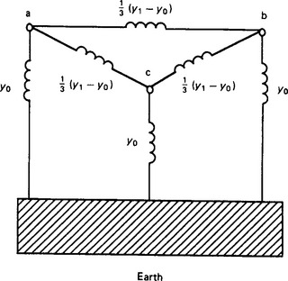
(h) Phase-shifting transformers: Phase-shifting transformers may be represented in a similar manner from an assembly of single-phase elements, but here the single-phase elements have to be derived.
(1) Single-phase equivalent-circuit model—following the method described in Section 3.3.5.2, the single-phase representation may be illustrated approximately as in Figure 3.59, where the ideal transformer now represents an ideal phase-shifting transformer. The invariance of the product V1* across the ideal transformer requires a distinction to be made between the turns ratios for current and voltage; thus
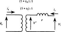
where 1 + tv = 1 + t + jq and 1 + t1 = 1 + t − jq.
Following the same procedure as before yields the 4 × 4 phase admittance matrix Y of the equivalent phase-shifting transformer. For a phase-shifting transformer, however, although an equivalent lattice network corresponding to the admittance matrix Y can be constructed, it is no longer a bilinear network because of asymmetry in Y. The equivalent circuit of a single-phase phase-shifting transformer is thus of limited value, and the transformer is best represented algebraically by its admittance matrix.
(2) Three-phase phase-shifting transformers—For both non-phase-shifting and phase-shifting transformers the phase-admittance matrix for any polyphase bank can be built up from the single-phase admittance matrices by identification of the nodes of each single-phase unit with the three-phase terminations, A, B, C and a, b, c according to the winding connection.
The three-phase admittance matrix of the star—delta phase-shifting transformer is:
The neutral node N has been preserved in the matrix. If N was earthed through an earthing impedance, the appropriate admittance would appear in the element yNN or, if earthed directly, the row and column corresponding to N would be removed.
3.3.5.2 Fault analysis
By representing polyphase network conditions in terms of their phase co-ordinates, i.e. phase voltages, currents and impedances, thereby preserving the physical identity of the system, instead of transforming the phase co-ordinates to symmetrical component co-ordinates, a generalised analysis of polyphase networks under all fault conditions can be developed.
General form of prefault equations: It was shown in Section 3.3.3.3 that the general form of the nodal admittance equations YV = I may be used to describe the three-phase system where each bus-bar in the one-line diagram of the balanced system is replaced by three equivalent separate-phase bus-bars. Each voltage and current element in equations YV = I for the balanced system is replaced correspondingly by three phase-to-earth voltages and three currents, with each element of the nodal-admittance matrix being replaced by a three-phase element represented by a 3 × 3 nodal admittance submatrix. The same principle used in the assembly of the single-phase admittance matrix underlies the assembly of the three-phase admittance matrix.
The phase relationships at each bus-bar are, then, at bus-bar k, for example,
where Ik is the phase current injected into bus-bar k, Vk is the phase-to-earth voltage, and Sk is the phase power.
The network admittance matrix Y can be adjusted to the basic prefault form from which all calculations for the various faults commence by classifying the energy sources as active or passive, according to their behaviour during fault conditions. Some loads, for example, may be characterised by passive admittances per phase; thus the equation for node j becomes
The network nodal admittance equations can be modified accordingly by substituting for the load currents and then transferring the admittances across to supplement the diagonal elements of matrix Y. If the load has unequal positive-negative-, and zero-sequence admittances, the admittance yj0′ may be replaced by an equivalent 3 × 3 phase admittance matrix, which in turn is transferred to supplement the appropriate block diagonal 3 × 3 submatrix of Y. In this case, the substitution for the three corresponding phase currents is made simultaneously.
With appropriate node connections, active sources such as machines may be represented by the general network element shown previously containing voltage sources in series with a passive network. The equations YV = I governing the current injected into the network from a star-connected machine connected to the three-phase bus-bars p, q, and r with a neutral earthed through an impedance yN0, are:
where IN is the current injected into the neutral node N, and is usually zero, EN is the sum of the phase e.m.f.s, and is also usually zero (Ep + Eq + Er = 0), y0 is the machine zero sequence admittance, y1 is the positive-sequence admittance, and YNN = 3y0 + yN0. The values of the voltage sources Ep, Eq and Er are the appropriate phase-displaced transient or subtransient values according to the purpose of the study.
Substituting again for the respective currents in equation YV = I and transferring the product terms yijVj to the left-hand side, the modified network admittance equations become
where Y′ is the supplemented phase admittance matrix and [ygE] or I′ is a column matrix the elements of which are of the form y1E, or zero. The similarity is evident between the three-phase prefault equations and the familiar equivalent one-line diagram or single-phase prefault equations established for three-phase fault studies of balanced systems described in Section 3.3.3.
Solution of equations for various types of fault condition: All the various types of fault condition can be analysed by means of simple modifications to, and the solution of, these equations.
(a) Single phase-to-earth fault: If a single phase-to-earth short circuit occurs at bus-bar k, the bus-bar voltage Vk will be constrained to be zero, the value of the earth reference voltage. To obtain the extra degree of freedom for this constraint to be valid within a consistent set of equations, the current on the right-hand side of the k th equation in equation (3.5) must be unspecified, and allowed to take its value according to the solution of the remaining set of (n − 1) equations in the (n − 1) unknown voltages, Vj, i = 1, 2, …, n, (i ≠ k), with Vk = 0.
Letting the value of this k th current be ![]() , where
, where
![]() is the prefault value and
is the prefault value and ![]() are the elements of the k th row of the matrix Y′, then ISC is the current in the short-circuit connection to earth.
are the elements of the k th row of the matrix Y′, then ISC is the current in the short-circuit connection to earth.
This calculation is exactly the same as that for a three-phase fault in existing computer programs based on a one-line diagram and three-phase apparent-power base.
The numerical methods of solution are the standard methods developed for such problems in linear algebra, namely matrix-inversion methods or, for large systems, iterative methods such as the Gauss—Seidel technique, and can be found in the usual numerical-analysis textbooks.
(b) Multiphase faults: These are described in (1)–(4) below.
(1) Phase-to-phase short circuits—for bus-bars short-circuited together (zero-impedance connection) either the modified admittance equations can be solved subject to a number of additional constraints, or the admittance matrix Y′ can be modified, and the number of equations reduced for solution without constraints.
In the first approach, where the number of nodes remains constant, the appropriate bus-bar voltages are constrained to be equal. To obtain the extra degrees of freedom for these constraints to be valid within a consistent set of equations, the currents on the right-hand sides of the corresponding equations must be unspecified and allowed to take their values accordingly. These currents are, at bus-bar k, for example,
where ΣISC is the total short-circuit current injected into bus-bar k from all other bus-bars short circuited to bus-bar k.
For a phase-to-phase short circuit occurring between bus-bars j and k, for example, the equations are solved with voltages Vj = Vk and currents I″j and I″k being unknown where
Ikj (= −Ijk) is the short-circuit current passing between bus-bars j and k, Ikj that being injected into bus-bar j, and Ijk being that injected into bus-bar k.
(2) Phase-to-phase faults via impedances—if the faults between phases occur through impedances the equations are solved for the voltages V with matrix Y′ supplemented by the appropriate admittances.
(3) Phase-to-phase-to-earth faults—earthed multiphase faults follow as extensions of the previous sections. If several phases are short circuited to earth simultaneously, the equations are solved with all the respective voltages having a value of zero. The total fault current to earth follows from the appropriate sums of the respective fault currents. If impedances are present in the fault, the corresponding admittances are included in the matrix Y′ and the fault currents are evaluated depending on the fault impedance configuration.
(4) Simultaneous faults—using phase co-ordinates, any two- or three-phase fault may be considered to be a multiple fault, in the sense that more than one represented bus-bar is involved. The techniques of solution above may be applied, therefore, without restriction, to any number of simultaneous faults, regardless of their type or geographical location. As noted previously, the solution involves the solving of a set of simultaneous linear algebraic equations with or without constraints on the appropriate voltages, depending on the modifications made to the original network connection table.
Open conductors: Open conductors present no difficulty other than that of introducing an extra bus-bar or bus-bars into the network, depending on the number of open circuits. The appropriate changes are made in the connection table, and the admittance or impedance matrices are modified accordingly.
The source transformation method of solution: The above methods of solution may be referred to as ‘distributed source methods’, in which the various equivalent-current sources retain their identity and are generalisations of the existing methods of solution in the standard three-phase fault-level analysis described in Section 3.3.3.2.
An alternative approach would be to use Norton’s theorem, or superposition methods, commencing from the supplemented nodal impedance matrix Z′ (= Y′−1). The method depends on knowing the voltage drop caused by the fault current, and hence determines this current for an equivalent current source acting alone at the point of fault. The fault conditions are then obtained by superposition.3
3.3.5.3 Polyphase loadflow analysis
For polyphase load flow, several questions are raised which are not encountered in balanced one-line diagram analysis. If the phase voltages are unbalanced then the characteristics of the loads under such conditions should be known. An admittance matrix representation may well be better than a specified P + jQ demand. A further problem is the lack of knowledge of the active and reactive power distribution between the phases of the generators.
A synchronous generator model avoiding this latter difficulty and using only the total output power of the machine is, for a machine connected to the three-phase bus-bars p, q and r:
To a first approximation the term yN0|VN|2/E*a can be neglected in comparison with the magnitude of the term ![]() .
.
For each generator the machine admittance matrix Yabc can be added to the polyphase admittance matrix representing the network of lines, transformers and admittance loads. By any of the usual load-flow techniques these equations can then be solved iteratively. At generator bus-bars where a P|V| specification is given, the value of P is the total active power output of the machine and |V| can be either Ea or Vp or any other controlled bus-bar voltage. Several existing conventional (one-line diagram) load-flow programs already allow the generator terminal voltage magnitude to be unknown and to be adjusted according to the voltage value of a remote-controlled bus-bar. In principle, the same situation and adjustments characterise the phase co-ordinate load-flow analysis
3.3.6 Network power limits and stability
Steady-state a.c. power transfer over transmission links has limitations imposed by terminal voltages and link impedance. Transient conditions for stable operation are dynamic, and more complicated.
3.3.6.1 Steady-state conditions
Two typical cases concern a link transferring power from a sending-end generator at bus-bar voltage Vs to a receiving end of voltage Vr where there is either (1) a static load only or (2) a generator. Case (2) is the more important, as loss of synchronism is possible.
(1) Load stability The power taken by a static load of constant power factor is proportional to the square of the voltage. As the load power is increased the voltage falls, at first slightly but subsequently more rapidly until maximum power is attained. Thereafter both load voltage and power decrease, but the system is still stable, though overloaded. The condition could occur following the clearance of a system fault.
The load is rarely purely static: it usually contains motors. With induction motors the reactive-power requirements increase as the voltage falls, and beyond the maximum-power conditions the machines will stall, and will draw heavy ‘pick-up’ currents after a restoration of the voltage.
(2) Synchronous stability The receiving-end active and reactive powers in terms of Vs and Vr, and the parameters ABCD, are given for a transmission link in Section 3.2.13.1. For a short line, A = 1 ∠0° and B = Z ∠ β, where Z = R + jX and β = arctan(X/R), conditions shown in Figure 3.27.
If the resistance R can be neglected (as is often the case, especially where the link includes terminal transformers), the receiving-end active power Pr and its maximum Prm become
To attain maximum active power, the receiving end must also accept a leading reactive power ![]() .
.
Interpreting the angle θ between Vs and Vr as that between the generator rotor (indicated by the e.m.f. E t) and Vr, and including the appropriate generator reactance in X, the angle is now the load angle δ, and maximum active power transfer will occur for a load angle δ = π/2 rad (90° electric). The relation for normal conditions is marked N in Figure 3.60.
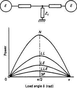
Although a system does not operate under continuous steady-state conditions with a system fault, the power—angle relation is important in the assessment of transient stability. The network for which the curve is calculated is obtained by connecting a ‘fault shunt’ Zf at the point of fault. The value of Zf is in terms of Z− and Z0, respectively, the total impedance to n.p.s. and z.p.s. currents up to the point of fault. These values are given below for line-line (LL), single-earth (LE), double-earth (LLE) and three-phase (3P) faults, while the corresponding power-angle relations are shown in Figure 3.60.
3.3.6.2 Transient conditions
If a system in a steady state is subjected to a sudden disturbance (e.g. short circuit, load change, switching out of a loaded circuit) the power demand will not immediately be balanced by change in the prime-mover inputs. To restore balance the rotors of the synchronous machines must move to new relative angular positions; this movement sets up angular oscillations, with consequent oscillations of current and power that may be severe enough to cause loss of synchronism. The phenomenon is termed transient instability.
Rotor angle: For a single machine connected over a transmission link to an infinite bus-bar, the simple system shown in Figure 3.61 applies. The mechanical input Pm is, in the steady state, balanced by the electrical output for the angle δ0 on the full-time power—angle relationship. If an electrical disturbance occurs such that the power—angle relation is suddenly changed to that indicated by the broken curve, the angle cannot immediately change because of the inertia of the generator and prime-mover rotors. The electrical power drops, and a power difference ΔP appears, accelerating the rotating members towards the new balancing angle δ1. Overshoot takes the rotor angle to δ2. If the disturbance is not severe, the rotor assumes the angle δ1 after some rapidly decaying oscillations of frequency 1 or 2 Hz. The angle—time relationship is that shown as curve A in Figure 3.62. However, if ΔP is large, the overshoot may cause loss of synchronism—the unstable curve B. A comprehensive investigation of stability thus involves the calculation of swing curves for the machines concerned.
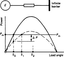
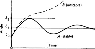
Equation of motion: The equation of motion for a single machine is
where M is the angular momentum. If the damping coefficients K1 and K2 are ignored, the equation of motion reduces to d2 δ2 δ/dt2 = Δ P/M.
A mass of inertia J rotating at angular speed ω stores a kinetic energy W = 1/2Jω2. The momentum M = Jω can be usefully related to the machine rating S by the inertia constant
in which ω1 is the synchronous angular speed (rad/s) and n1 = ω1/2π = f/p is the corresponding rotational speed (revolutions per second) for a machine with 2p poles operating at a frequency f. The magnitude of H (in joules/volt-ampere, or MJ/MV-A, or seconds) has the typical values given in Table 3.11.
Table 3.11
Inertia constants of 50 Hz synchronous machines
| Machine | n (rev/s) | H (s) |
| Turbogenerators | 50 | 3–7 |
| 25 | 5–10 | |
| Compensators | — | 1–1.25 |
| Motors | — | 2–2.25 |
| Hydrogenerators | 8.3 | 2–4 |
| 5 | 2–3.5 | |
| 2.5 | 2–3 | |
| 1.7 | 15–2.5 |
A direct solution of the equation of motion is not normally possible, and a step-by-step process must be adopted. For this, a succession of time intervals (e.g. 50 ms) is selected and the rotor acceleration (d2δ/dt2) is calculated at the beginning of each. Assuming the acceleration to be constant throughout a time interval, the angular velocity and the movement δ during the interval can be found. At the end of the first interval, the new ΔP is obtained from the power—angle curve and used to calculate the acceleration during the second interval, and so on. The complete swing curve can thus be obtained. The method can be extended (if the relevant data are available) to include damping, changes in excitation, saliency, prime-mover governor action and other factors that affect the swing phenomenon.
Multi-machine system A two-machine system with a transmission link can be represented by a single machine feeding an infinite bus-bar and having an equivalent momentum M = M1M2/(M1 + M2).
A group of machines 1, 2, …, paralleled on the same bus-bar can be treated as a single machine of rating S = S1 + S2 + …, and of equivalent momentum M = (S1/S) M1 + (S2/S)M2 + ….
For a multi-machine network, a separate equation of motion must be set up for each generator and a step-by-step solution undertaken. Determination of ΔP for each machine at the end of a time interval involves a comprehensive load-flow calculation by computer.
Equal-area criterion: Neglecting damping, governor action and changes in excitation, the stability of a simple generator/link/infinite-bus-bar system can be checked graphically using power-angle relationships. Consider the system shown in Figure 3.63, with the generator operating at a load angle δ0 on the power—angle curve P2 with a prime-mover input Pm and both transmission links intact. A fault occurs on one link, changing the power—angle relationship to Pf and giving a power difference ΔP between Pm and the electrical output. As a result the rotor accelerates until the angle δs is reached, when the faulted link is switched out. The kinetic energy acquired by the rotor during this period is represented by area A. At δs the power—angle relationship becomes P1 corresponding to a single healthy link. This reverses ΔP and the rotor decelerates. At the angle δ2 such that area B (representing kinetic energy returned from the rotor) is equal to A, the rotor speed is again synchronous. However, ΔP is now reversed and the rotor will begin to swing back. The range of rotor-angle excursions is stable, but there is a critical value of the fault-clearance angle δs that, if exceeded, will result in instability. If all the power—angle relationships are true sinusoids, the critical angle can be found analytically.
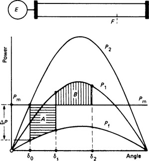
Conditions other than that shown in Figure 3.63 can be dealt with if the relevant power—angle relationships can be drawn. It is to be noted that a swing curve may be required to relate rotor angle to time, as it is the time of fault clearance (or other event)—a quantity based on the delay of switch opening—that is normally specified.
1. Electrical Transmission and Distribution Reference Book. Westinghouse Electric Corporation; 1950.
2. Part 1 Laughton, M.A., Analysis of unbalanced polyphase networks by the method of phase co-ordinates. System representation in phase frame of reference. Proc IEE., 115. Aug 1968:1163–1172.
3. Laughton, M.A., Analysis of unbalanced polyphase networks by the method of phase co-ordinates. Part 2 Fault analysis. Proc IEE., 116. 1969:857–865.
4. Laughton, M.A., Saleh, A.O.M. Unified phase co-ordinate loadflow and fault analysis of polyphase networks. Elec Power Energy Systems J.. Oct 1980;2(4):181–192.
5. Saleh, A.O.M., Laughton, M.A., Stone, G.T. M- to N-phase transformer models in phase coordinates. Proc IEE, Part C. Jan 1985;132:41–48.
6. Saleh, A.O.M., Laughton, M.A. Phase co-ordinate and fault analysis program. Elec Power Energy Systems J.. Oct 1980;2(4):193–200.