Programmable Controllers
16.1 Introduction
16.1.1 The computer in control
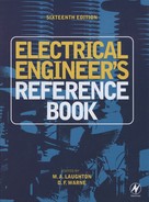
A computer can be considered as a device that follows predetermined instructions to manipulate input data in order to produce new output data as summarised on Figure 16.1(a). Early computer systems tended to be based on commercial functions; payroll, accountancy, banking and similar activities. The operations tended to be batch processes; a daily update of stores stock for example.
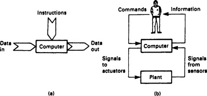
Figure 16.1 The computer as part of an industrial control system: (a) a simple overview of a computer; (b) the computer as part of a control system
A computer can also be used as part of a control system as Figure 16.1(b). The input data will be the operator’s commands and signals from the plant (limit switches, flows, temperatures). The output data are control actions to the plant and status displays to the operator. The instructions will define what action is to be taken as the input data (from both the plant and the operator) changes.
The first industrial computer application was probably a system installed in an oil refinery in Port Arthur USA in 1959. The reliability and mean time between failure of computers at this time meant that little actual control was performed by the computer, and its role approximated to a simple monitoring subsystem.
16.1.2 Requirements for industrial control
Industrial control has rather different requirements than other computer applications. It is worth examining these in some detail.
A conventional computer takes data, usually from a keyboard, and outputs data to a screen or printer. The data being manipulated will generally be characters or numbers (e.g. item names and quantities held in a stores stock list).
An industrial control computer is very different. Its inputs come from a vast number of devices. Although some of these will be numeric (flows, temperature, pressures and similar analog signals) the majority will be single bit, on/off, digital signals representing valves, limit switches, motor contactors etc.
There will also be a similar large amount of digital and analog output signals. A very small control system may have connections to about twenty input and output signals; figures of over two hundred connections are quite common on medium sized systems.
Although it is possible to connect this quantity of signals into a conventional machine, it requires non-standard connections and external boxes. Similarly, although programming for a large amount of input and output signals can be done in Pascal, BASIC or C, the languages are being used for a purpose for which they were not really designed, and the result can be very ungainly.
In Figure 16.2(a), for example, we have a simple motor starter. This could be connected as a computer driven circuit as Figure 16.2(b). The two inputs are identified by addresses 1 and 2, with the output (the relay starter) being given the address 10.
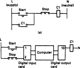
Figure 16.2 Comparison of hardwire and computer based systems: (a) hardwire motor starter; (b) computer based motor starter
If we assume a program function bitread (N) exists which gives the state (on/off) of address N, and a function bitwrite (M, var) which sends the state of program variable var to address M, we could give the actions of Figure 16.2 by where start, stop and run are one bit variables. The program is not very clear, however, and we have just three connections.
An industrial control program rarely stays the same for the whole of its life. There are always modifications to cover changes in the operations of the plant. These changes will be made by plant maintenance staff, and must be made with minimal (preferably none) interruptions to the plant production. Adding a second stop button and a second start button into Figure 16.2 would not be a simple task.
In general, computer control is done in real time, i.e. the computer has to respond to random events as they occur. An operator expects a motor to start (and more important to stop!) within a fraction of a second of a button being pressed. Although commercial computing needs fast computers, it is unlikely that the difference between a one second and two second computation time for a spreadsheet would be noticed by the user. Such a difference would be unacceptable for industrial control.
Time itself is often part of the control strategy (e.g. start air fan, wait 10 secs for air purge, open pilot gas valve, wait 0.5 s, start ignition spark, wait 2.5 s, if flame present open main gas valve). Such sequences are difficult to write with conventional languages.
Most control faults are caused by external items (limit switches, solenoids and similar devices) and not by failures within the central control itself. The permission to start a plant, for example, could rely on signals involving cooling water flows, lubrication pressure and temperatures all being within allowable ranges. For quick fault finding the maintenance staff must be able to monitor the action of the computer program whilst it is running. If, as is quite common, there are ten interlock signals which allow a motor to start, the maintenance staff will need to be able to check these quickly in the event of a fault. With a conventional computer, this could only be achieved with yet more complex programming.
The power supply in an industrial site is shared with many antisocial loads; large motors stopping and starting, thyristor drives which put spikes and harmonic frequencies onto the mains supply. To a human these are perceived as light flicker; to a computer they can result in storage corruption or even machine failure.
An industrial computer must therefore be able to live with a ‘dirty’ mains supply, and should also be capable of responding sensibly following a total supply interruption. Some outputs must go back to the state they were in before the loss of supply, others will need to turn off or on until an operator takes corrective action. The designer must have the facility to define what happens when the system powers up from cold.
The final considerations are environmental. A large mainframe computer generally sits in an air conditioned room at a steady 20°C with carefully controlled humidity. A desk top PC will normally live in a fairly constant office environment because human beings do not work well at extremes. An industrial computer, however, will probably have to operate away from people in a normal electrical substation with temperatures as low as −10°C after a winter shutdown, and possibly over 40°C in the height of summer. Even worse, these temperature variations lead to a constant expansion and contraction of components which can lead to early failure if the design has not taken this factor into account.
To these temperature changes must be added dust and dirt. Very few industrial processes are clean, and the dust gets everywhere. The dust will work itself into connectors, and if these are not of a highest quality, intermittent faults will occur which can be very difficult to find.
In most computer applications, a programming error or a machine fault can often be humorous (bills and reminders for Op) or at worse expensive and embarrassing. When a computer controlling a plant fails, or a programmer misunderstands the plants operation, the result could be injuries or fatalities. It behoves everyone to take extreme care with the design.
Our requirements for industrial control computers are very demanding, and it is worth summarising them:
• They should be designed to survive in an industrial environment with all that this implies for temperature, dirt and poor quality mains supply.
• They should be capable of dealing with bit form digital input/output signals at the usual voltages encountered in industry (24 V d.c. to 240 V a.c.) plus analog input/output signals. The expansion of the I/O should be simple and straightforward.
• The programming language should be understandable by maintenance staff (such as electricians) who have no computer training. Programming changes should be easy to perform in a constantly changing plant.
• It must be possible to monitor the plant operation whilst it is running to assist fault finding. It should be appreciated that most faults will be in external equipment such as plant mounted limit switches, actuators and sensors, and it should be possible to observe the action of these from the control computer.
• The system should operate sufficiently fast for real-time control. In practice, ‘sufficiently fast’ means a response time of around 0.1 sec, but this can vary dependent on the application and the controller used.
16.1.3 Enter the PLC
In the late 1960s the American motor car manufacturer General Motors was interested in the application of computers to replace the relay sequencing used in the control of its automated car plants. In 1969 it produced a specification for an industrial computer similar to that outlined at the end of the previous section.
Two independent companies, Bedford Associates (later called Modicon) and Allen Bradley (now owned by Rockwell) responded to General Motors specifications. Each produced a computer system similar to Figure 16.3 which bore little resemblance to the commercial minicomputers of the day.
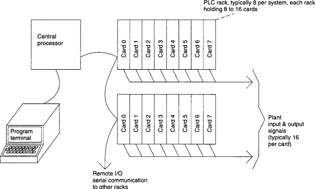
The computer itself, called the central processor, was designed to live in an industrial environment, and was connected to the outside world via racks into which input, or output cards could be plugged.
Each input or output card could connect to 16 signals. A typical rack would contain eight cards and the processor could connect to eight racks, allowing connection to 1024 devices. It is very important to appreciate that the card allocations were the user’s choice, allowing great flexibility.
The most radical idea, however, was a programming language based on a relay schematic diagram, with inputs (from limit switches, pushbuttons, etc.) represented by relay contacts, and outputs (to solenoids, motor starters, lamps, etc.) represented by relay coils. Figure 16.4(a) shows a simple hydraulic cylinder which can be extended or retracted by pushbuttons. Its stroke is set by limit switches which open at the end of travel, and the solenoids can only be operated if the hydraulic pump is running. This would be controlled by the computer program of Figure 16.4(b) which is identical to the relay circuit needed to control the cylinder. These programs look like the rungs on a ladder, and were consequently called ‘Ladder Diagrams’.
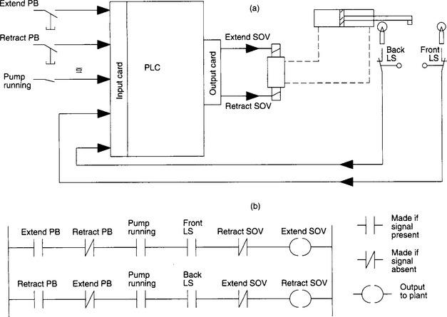
Figure 16.4 A simple PLC application: (a) a hydraulic cylinder controlled by a PLC; (b) the ‘Ladder Diagram’ program used to control the cylinder
The program was entered via a programming terminal with keys showing relay symbols (normally open/normally closed contacts, coils, timers, counters, parallel branches, etc.), with which a maintenance electrician would be familiar. Figure 16.5 shows the programmer’s keyboard for an early PLC. The meaning of the majority of the keys should be obvious to any maintenance electrician. The program, shown exactly on the screen as Figure 16.4(b), would highlight energised contacts and coils allowing the programming terminal to be used for simple faultfinding.

Figure 16.5 A programming keyboard from an early PLC programming terminal. The link between the keys and relay symbols can be clearly seen. Figure courtesy of Allen Bradley
The name given to these machines was Programmable Controllers or PCs. The name Programmable Logic Controller or PLC was also used, but this is, strictly, a registered trade mark of the Allen Bradley Company, now part of Rockwell. Unfortunately in more recent times the letters PC have come to be used for Personal Computer, and confusingly the worlds of programmable controllers and personal computers overlap where portable and lap-top computers are now used as programming terminals. To avoid confusion, we shall use PLC for a programmable controller and PC for a personal computer.
16.1.4 The advantages of PLC control
Any control system goes through several stages from conception to a working plant.
The first stage is Design when the required plant is studied and the control strategies decided. With conventional systems every ‘i’ must be dotted before construction can start. With a PLC system all that is needed is a possibly (usually!) vague idea of the size of the machine and the I/O requirements (so many inputs and outputs). The cost of the input and output cards are cheap at this stage, so a healthy spare capacity can be built in to allow for the inevitable omissions and future developments.
Next comes Construction. With conventional schemes, every job is a ‘one-off’ with inevitable delays and costs. A PLC system is simply bolted together from standard parts.
The next stage is Installation, a tedious and expensive business as sensors, actuators, limit switches and operator controls are cabled. A distributed PLC system (discussed in Section 16.5) using serial links and pre-built and tested desks can simplify installation and bring huge cost benefits. The majority of the PLC program is usually written at this stage.
Finally comes Commissioning, and this is where the real advantages are found. No plant ever works first time. Human nature being what it is, there will be some oversights. (We need a limit switch to only allow feeding when the discharge valve is ‘shut’ or ‘Whoops, didn’t we say the loading valve is energised to UNLOAD on this system’ and so on.) Changes to conventional systems are time consuming and expensive. Provided the designer of the PLC systems has built in spare memory capacity, spare I/O and a few spare cores in multi-core cables, most changes can be made quickly and relatively cheaply. An added bonus is that all changes are inherently recorded in the PLC’s program and commissioning modifications do not go unrecorded.
There is an additional fifth stage called Maintenance which starts once the plant is working and is handed over to production. All plants have faults, and most tend to spend the majority of their time in some form of failure mode. A PLC system provides a very powerful tool for assisting with fault diagnosis.
A plant is also subject to many changes during its life to speed production, ease breakdowns or because of changes in its requirements. A PLC system can be changed so easily that modifications are simple and the PLC program will automatically document the changes that have been made.
16.2 The programmable controller
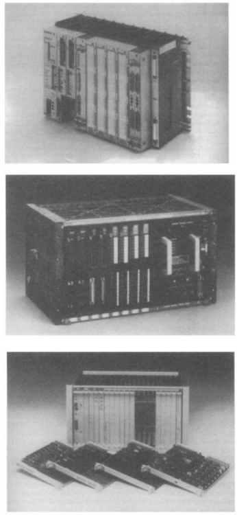
This chapter is written around five manufacturers’ ranges:
• The Allen Bradley PLC-5 series. Allen Bradley, now owned by Rockwell, were one of the original PLC originators (and actually has the US copyright on the name PLC). They have been responsible for much of the development of the ideas used in PLCs and have succeeded in maintaining a fair degree of upward compatibility from their earliest machine without restricting the features of the latest.
• The Siemens Simatic 55 range which is probably the commonest PLC in mainland Europe.
• The British GEM-80, originally designed by GEC from a long association with industrial computers dating back to English Electric. This part of GEC is now known as CEGELEC and is part of a French group in which Alsthom are a major shareholder.
• The ASEA Master System, now manufactured by the ABB company formed by the merger of ASEA and Brown Boveri. The Master system has features more akin to a conventional computer system and its programming language has some interesting and powerful features.
The above four PLCs are shown on Figure 16.6. Many PLC systems are now very small and as an example of this bottom end of the market we shall also consider the Japanese Mitsubishi F2-40.
16.2.2 I/O connections
Internally a computer usually operates at 5 V d.c. The external devices (solenoids, motor starters, limit switches, etc.) operate at voltages up to 110 V a.c. The mixing of these two voltages will cause irreparable damage to the PLC electronics. A less obvious problem can occur from electrical ‘noise’ introduced into the PLC from voltage spikes, caused by interference on signals lines, or from load currents flowing in a.c. neutral or d.c. return lines. Differences in earth potential between the PLC cubicle and outside plant can also cause problems.
There are obviously very good reasons for separating the plant supplies from the PLC supplies with some form of barrier to ensure that the PLC cannot be adversely affected by anything happening on the plant. Even a cable fault putting 415 V a.c. onto a d.c. input would only damage the input card; the PLC itself (and the other cards in the system) would not suffer.
This isolation is achieved by optical isolators consisting of a linked light emitting diode and photoelectric transistor. When current is passed through the diode it emits light causing the transistor to switch on. Because there is no electrical connections between the diode and the transistor, very good electrical isolation (typically 1-4 KV) is achieved.
A d.c. input can be provided as Figure 16.7(a). When the push button is pressed, current will flow through D1 causing TR1 to turn on passing the signal to the PLC internal logic. Diode D2 is a light emitting diode used as a fault finding aid to show when the input signal is present. Such indicators are present on almost all PLC input and output cards. The resistor R sets the voltage range of the input. D.c. input cards are usually available for three voltage ranges; 5 V (TTL), 12–24V, 24–50V.
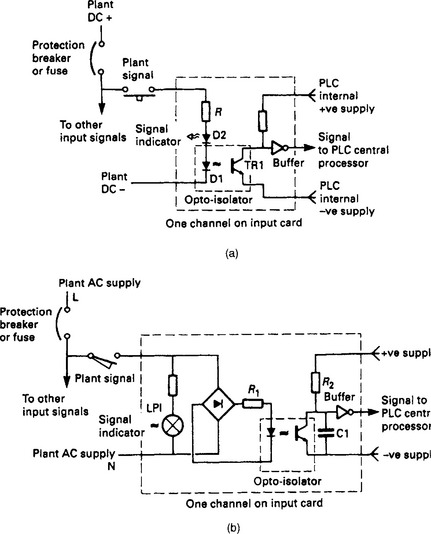
A possible a.c. input circuit is shown on Figure 16.7(b). The bridge rectifier is used to convert the a.c. to full wave rectified d.c. Resistor R2 and capacitor C1 act as a filter (typically 50 ms time constant) to give a clean signal to the PLC logic. As before a neon LP1 acts as an input signal indicator for fault finding, and resistor R1 sets the voltage range.
Output connections also require some form of isolation barrier to limit damage from the inevitable plant faults and to stop electrical ‘noise’ corrupting the processor’s operations. Interference can be more of a problem on outputs because higher currents are being controlled by the cards and the loads (solenoids and relay coils) are often inductive.
In Figure 16.8, eight outputs are fed from a common supply, which originates local to the PLC cubicle (but separate from the supply to the PLC itself). This arrangement is the simplest and the cheapest, to install. Each output has its own individual fuse protection on the card and a common circuit breaker. It is important to design the system so that a fault, say, on load 3 blows the fuse FS3 but does not trip the supply to the whole card shutting down every output. This is known as ‘discrimination’.
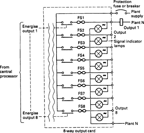
Contacts have been shown on the outputs in Figure 16.8. Relay outputs can be used (and do give the required isolation) but are not particularly common. A relay is an electromagnetic device with moving parts and hence a finite limited life. A purely electronic device will have greater reliability. Less obviously, though, a relay driven inductive load can generate troublesome interference and lead to early contact failure.
A transistor output circuit is shown on Figure 16.9(a). Opto-isolation is again used to give the necessary separation between the plant and the PLC system. Diode D1 acts as a spike suppression diode to reduce the voltage spike encountered with inductive loads as shown on Figure 16.9(b). The output state can be observed on LED1. Figure 16.9(a) is a current sourcing output. If NPN transistors are used, a current sinking card can be made as Figure 16.9(c).
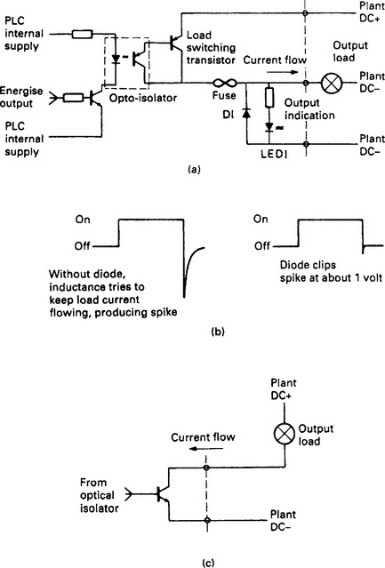
Figure 16.9 D.c. output circuits: (a) isolated output circuit, current sourcing; (b) the effect of an inductive load and the reason for including diode D1; (c) current sinking output
A.c. output cards invariably use triacs. a typical circuit being shown on Figure 16.10. Triacs have the advantage that they can be made to turn on at zero voltage and inherently turn off at zero current in the load. The zero current turn off eliminates the spike interference caused by breaking the current through an inductive load. If possible, all a.c. loads should be driven from triacs rather than relays.
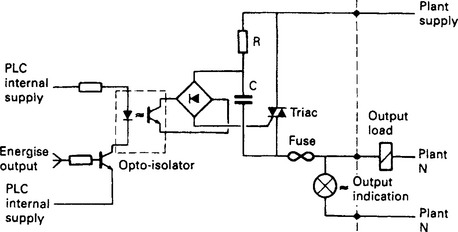
Figure 16.10 A.c. isolated output. The triac switches on at zero voltage and off at zero current which minimises interference
An output card will have a limit to the current it can supply, usually set by the printed circuit board tracks rather than the output devices. An individual output current will be set for each output (typically 2 A) and a total overall output (typically 6 A). Usually the total allowed for the card current is lower than the sum of the allowed individual outputs.
16.2.3 Remote I/O
So far we have assumed that a PLC consists of a processor unit and a collection of I/O cards mounted in local racks. Early PLCs were arranged like this, but in a large and scattered plant, all signals had to be brought back to some central point in expensive multi-core cables. This also makes commissioning and fault finding rather difficult, as signals can only be monitored effectively at a point distant from the plant device being tested.
In all bar the smallest and cheapest systems, PLC manufacturers therefore provide the ability to mount I/O racks remote from the processor, and linked with simple (and cheap) screened single pair or fibre optic cable. Racks can then be mounted up to several kilometres away from the processor.
There are many benefits from this. It obviously reduces cable costs as racks can be laid out local to the plant devices and only short multi-core cable runs are needed. The long runs will only be the communication cables (which are cheap, easy to install and only have a few cores to terminate at each end) and hardwire safety signals.
Less obviously, remote I/O allows complete plant units to be constructed, wired to a built in PLC rack, and tested off site prior to delivery and installation. Typical examples are hydraulic skids, desks and even complete control pulpits. The use of remote I/O in this way can greatly reduce installation and commissioning time and cost.
The use of serial communication for remote I/O means some form of sequential scan must be used to read input and update outputs. This scan, typically 30–50 ms, introduces a small delay in the response to signals discussed further in the following section.
If remote I/O is used, provision should be made for a program terminal to be connected local to each rack. It negates most of the benefits if the designer can only monitor the operation from a central control room several hundred metres from the plant. Fortunately, manufacturers have recognised this and most PLCs have programming terminals which can be remotely connected to the processor.
16.2.4 The program scan
A PLC program can be considered to behave as a permanent running loop similar to Figure 16.11(a). The user’s instructions are obeyed sequentially, and when the last instruction has been obeyed the operation starts again at the first instruction. A PLC does not, therefore, communicate continuously with the outside world, but acts, rather, by taking ‘snapshots’.
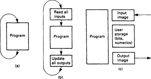
Figure 16.11 The program scan and memory organisation: (a) simple view of PLC operation; (b) more detailed view of PLC operation; (c) memory organisation
The action of Figure 16.11(a) is called a program scan, and the period of the loop is called the program scan time. This depends on the size of the PLC program and the speed of the processor, but is typically 2–5 ms per K of program. Average scan times are usually around 10–50 ms.
Figure 16.11(a) can be expanded to Figure 16.11(b). The PLC does NOT read inputs as needed (as implied by Figure 16.11(a)) as this would be wasteful of time. At the start of the scan it reads the state of ALL the connected inputs and stores their state in the PLC memory. When the PLC program accesses an input, it reads the input state as it was at the start of the current program scan.
As the PLC program is obeyed through the scan, it again does not change outputs instantly. An area of the PLC’s memory corresponding to the outputs is changed by the program, then ALL the outputs are updated simultaneously at the end of the scan. The action is thus:Read Inputs,Scan Program,Update Outputs.
The PLC memory can therefore be considered to consist of four areas as shown on Figure 16.11(c). The inputs are read into an input mimic area at the start of the scan, and the outputs updated from the output mimic area at the end of the scan. There will be an area of memory reserved for internal signals which are used by the program but are not connected directly to the outside world (timers, counters, storage bits (e.g. fault signals) and so on). These three areas are often referred to as the data table (Allen Bradley) or the database (ASEA/ABB).
This data area is smaller than may be at first thought. A medium size PLC system will have around 1000 inputs and outputs. Stored as individual bits in a PLC with a 16 bit word this corresponds to just over 60 storage locations. An analog value read from the plant or written to the plant will take one word. Timers and counters take two words (one for the value, and one for the preset) and sixteen internal storage bits take just one word. The majority of the store therefore, is taken up by the fourth area, the program itself.
The program scan limits the speed of signals to which a PLC can respond. In Figure 16.12(a) a PLC is being used to count a series of fast pulses, with the pulse rate slower than the scan rate. The PLC counts correctly. In Figure 16.12(b) the pulse rate is faster than the scan rate and the PLC starts to miscount and miss pulses. In the extreme case of Figure 16.12(c) whole blocks of pulses are totally ignored.

In general, any input signal a PLC reads must be present for longer than the scan time; shorter pulses may be read if they happen to be present at the right time but this cannot be guaranteed. If pulse trains are being observed, the pulse frequency must be slower than 1/(2 × scan period). A PLC with a scan period of 40 ms can, in theory, just about follow a pulse train of 1/(2 × 0.04) = 12.5 Hz. In practice other factors such as filters on the input cards have a significant effect and it always advisable to be conservative in speed estimates.
Less obviously, the PLC scan can cause a random ‘skew’ between inputs and outputs. In Figure 16.13 an input I is to cause an ‘immediate’ output O. In the best case of Figure 16.13(a), the input occurs just at the start of the scan, resulting in the energisation of the output one scan period later. In Figure 16.13(b) the input has arrived just after the inputs are read, and one whole scan is lost before the PLC ‘sees’ the input, and the rest of the second scan passes before the output is energised. The response can thus vary between one and two scan periods.
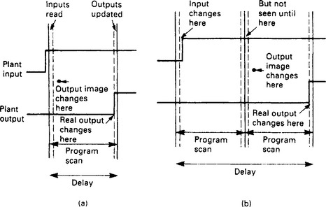
In the majority of applications this skew of a few tens of milliseconds is not important (it cannot be seen, for example, in the response of a plant to pushbuttons). Where fast actions are needed, however it can be crucial. If, for example, material travelling at 15 m/s is be cut to length by a PLC with the cut being triggered by a photocell a 30 ms scan time would result in a 0.03 × 15 000 = 450 mm variation in cut length.
PLC manufacturers provide special cards (which are really small processors in their own right) for dealing with this type of high speed application. We will return to these later in Section 16.4.8
The layout of the PLC program itself can result in undesirable delays if the program logic flows against the PLC program scan. The PLC starts at the first instruction for each scan, and works its way through the instructions in a sequential manner to the end of the program when it does its output update, then goes to read its inputs and run through the program again.
In Figure 16.14(a), an input I again causes an output O, but it goes through five steps first (it could be stepping a counter or seeing if some other required conditions are present). The program logic, however, is flowing against the scan. On the first scan the input I causes event A. On the next scan event A causes event B and so on until after 5 scans event D causes the output to energise. If the program had been arranged as Figure 16.14(b) the whole sequence would have occurred in one single scan.
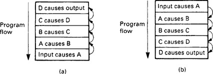
Figure 16.14 Compounding of program scan delays: (a) logic flows against the scan, five scan times from input to output; (b) logic flows with program scan, output occurs in same program scan as input
The failings of Figure 16.14(a) are self-evident, but the effect can often occur when the layout of the program is not carefully planned. The effect can also be used deliberately to ensure sequences operate correctly.
The effect of scan times can become even more complex when remote serially scanned I/O racks are present. These are generally read by an I/O scanner as Figure 16.15 but the remote I/O scan is not usually synchronised to the program scan. In this case with, say, a program scan of 30 ms and a remote I/O scan of 50 ms the fastest response to an input could be 30 ms, but the slowest response (with an input just missing the I/O scan and the I/O scan just missing the program scan and the programming scan just missing the I/O scan to update the output) could be 180 ms.
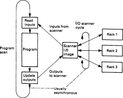
Figure 16.15 The effect of remote input/output scan times. The remote I/O scan usually free-runs and is not synchronised with the program scan
PLC manufacturers offer many facilities to reduce the effect of scan times. Typical are intelligent high speed independent I/O cards and the ability to sectionalise the program into areas with different scan rates.
16.3 Programming methods
The programming language of a PLC will be used by engineers, technicians and maintenance electricians. It should therefore be based on techniques used in industry rather than techniques used in computer programming. In this section we shall look at the various ways of programming PLCs from different manufacturers.
16.3.2 I/O identification
The PLC program is concerned with connections to the outside plant, and these input and output devices need to be identified inside the program. Before we can examine how the program is written we will first discuss how various manufacturers treat the I/O.
The earlier Figure 16.3 showed that a medium sized PLC system consists of several racks each containing cards, with each card interfacing generally with 8, 16 or 32 devices. I/O addressing is usually based on this rack/card/bit idea.
The Allen Bradley PLC-5 family has a range of processors which can address up to 64 racks. Its medium size 5/25 can have up to 8 racks. The rack containing the processor is automatically defined as rack 0, but the designer can allocate addresses of the other racks (in the range 1–7) by set up switches. The racks other than rack 0 connect to the processor via a remote I/O serial communications cable.
Each rack contains 16 card positions which are grouped in pairs called a ‘slot’. A 16 card rack thus contains eight slots, numbered 0–7. A slot can contain one 16 way input card and one 16 way output card OR two 8 way cards usually (but not necessarily) of the same type.
with bit being 2 digits. Allen Bradley use octal addressing for bits, so allowable numbers are 00–07 and 10–17. The address 1: 27/14 is input 14 (octal remember) on slot 7 in rack 2.
Outputs are addressed in a similar manner:
so O : 35/06 is output 6 in slot 5 of rack 2. Note that if 16 way cards are used an input and an output can have the same rack/slot/bit address, being distinguished only by the I: or the O:. With 8 way cards there can be no sharing or rack/slot/bit addressing.
The digital I/O in Siemens 115 PLCs is arranged into groups of 8 bits, called a Byte. A signal is identified by its bit number (0–7) and its byte number (0–127).
I9.4 is thus an input with bit address 4 in byte 9, and Q63.6 is an output with bit address 6 in byte 63.
Like Allen Bradley, Siemens use card slots in one or more racks. The cards are available in 16 bit (2 byte) or 32 bit (4 byte) form. A system can be built with local racks connected via a parallel bus cable or as remote racks with a serial link.
The simplest form of addressing is fixed slot where four bytes are assigned sequentially to each slot; 0–3 to the first slot, 4–7 to the next slot and so on. Input 112.4 is thus input bit 4 on the first byte of the card in slot 3 of the first rack. If 16 bit (2 byte) cards are used with fixed (4 byte) addressing the upper 2 bytes in each slot are lost.
In all bar the simplest system the user has the ability to assign byte addresses. This is known as variable slot addressing. The first byte address and the range (2 byte for 16 bit cards or 4 byte for 32 bit cards) can be set independently for each slot by switches in the adaptor module in each rack. Although any legitimate combination can be set up, it is recommended that a logical order is used.
Siemens use different notations in different countries with multi-lingual programming terminals. A common European standard is German, where E (for Eingang or input) is used for inputs (e.g. E4.7) and A (for Ausgang) used for outputs (e.g. A3.5).
The GEM-80 again configures its I/O in terms of bits and slots within racks. The processor rack can contain 8 card positions, and additional I/O can be connected into 12 position racks local to the processor connected via ribbon cable (called Basic I/O) or remotely via a serial link.
The I/O is addressed in terms of 16 bit words, one word corresponding to one or two card positions, and the prefix A being used for inputs and B for outputs. The bit addressing runs in decimal from 0 to 15.
A3 · 12 is thus input bit 12 in word 3 and B5 · 0 4 is output bit 4 in word 5
A word can only be an input or an output; duplication of word addresses is not allowed. I/O cards are available in 8 bit, 16 bit and 32 bit form, so one slot can be half a word, one word or two words according to the cards being used. Individual slot addresses are set by rotary switches on the back plane of each rack. The user has a more or less free choice in this allocation, but as usual it is best to use a logical sequential progression.
The ABB (originally ASEA) Master system is a more complex system than any we have discussed so far. Its organisation brings the user closer to the computer, and its language is more akin to the ideas used by programmers. If the PLCs discussed so far are taken to be represented by the home computer language BASIC, the ABB Master is analogous to PASCAL or C. This comparison is actually closer than might, at first, be thought. BASIC is quick and easy to use, but can de-generate into a web of spaghetti programming if care is not taken. PASCAL and C are more powerful but everything has to be declared and the language forces organisation and structure on the user.
The I/O cards are NOT identified by position in the rack, but by an address set on the card by a small plug with solder links. The I/O addressing does not, therefore, relate to card position, and a card can, in theory, be moved about without changing its operation.
The processor memory is arranged as Figure 16.16(a). The I/O is connected to a processor database, but unlike PLCs described earlier, the designer can specify different scan rates for different cards.
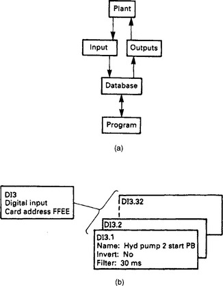
Figure 16.16 The ABB Master system: (a) organisation of the memory; (b) definition of a digital input in the database
The designer also has considerable power over how the PLC program is organised. This is heavily modularised as we shall see later, and the user can also specify different scan rates for different modules of the program.
Figure 16.16(b) indicates the database for one input card. There are two levels of the definition, the top level relating to details of the board itself such as address and scan rate, then lower levels relating to details of each channel on the board such as its name and whether the signal is to be inverted. The database holds details for all the I/O which can then be referenced by the program either by its database identification (e.g. DI3.1) or by its unique name (e.g. HydPump2StartPB).
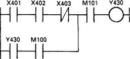
The Mitsubishi F2 range is typical of small PLCs with input/output connection, power supply and processor all contained in one unit. The smallest unit, the F2-40 M has 24 inputs and 16 outputs. (It is a characteristic of process control systems that the ratio input:outputs is generally 3:2.)
The 24 inputs are designated X400–X427 in octal notation and the 16 outputs Y430–Y447. The apparently arbitrary numbers are directly related to the storage locations used to hold the image of the inputs and output. Further addresses are used in larger PLCs in the series.
16.3.3 Ladder logic
Early PLCs, designed for the car industry, replaced relay control schemes. The symbols used in American relay drawings, -] [- for a normally open (NO) contact, -] / [- for a normally closed (NC) contact, and − ( ) − for a plant output, were the basis of the language. The earlier Figure 16.5 showed the keyboard for a programmer for this type of PLC; the relationship to relay symbolism is obvious.
Suppose we have a hydraulic unit, and we wish to give a healthy lamp indication when
The Pump is running (sensed by an auxiliary contact on the pump starter).
There is oil in the tank (sensed by a level switch which makes for good level).
There is oil pressure (sensed by a pressure switch which makes for adequate pressure).
With conventional relays, we would wire up a circuit as Figure 16.17(a).
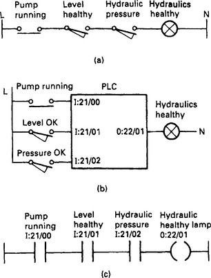
Figure 16.17 From a relay circuit to a PLC program: (a) basic non PLC circuit; (b) wiring of I/O to a PLC; (c) the corresponding PLC program
To use a PLC, we connect the input signals to an input card, and the lamp to an output card as Figure 16.17(b). The I/O notation used is Allen Bradley.
The program to provide the function is shown on Figure 16.17(c). The line on the left can be considered to be a supply, and the line on the right a neutral. The output is represented by a coil − ( ) − and is energised when there is a route from the left-hand rail. Output 0:22/01 will come on when signals I:21/00, I:21/01 and I:21/02 are all present.
The program is entered from a terminal with keys representing the various relay symbols. The terminal can also be used to monitor the state of the inputs and outputs, with ‘energised’ inputs and outputs being shown highlighted on the screen.
In Figure 16.18(a), a hydraulic cylinder can be extended or retracted by operation of two pushbuttons. The notation this time is for a GEM-80. It is undesirable to allow both solenoids to be operated together; this will almost certainly result in blown fuses in the supply to the output card, so some protection is needed. The program to achieve this is shown on Figure 16.18(b).
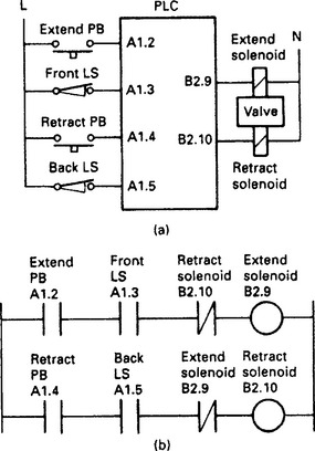
Figure 16.18 Ladder diagram in GEM-80 notation: (a) input/output connections; (b) GEM-80 ladder diagram
Normally closed contacts -] / [- have been used here. Output B2.9, the extend solenoid, will be energised when the extend pushbutton is pressed, providing the retract solenoid is not energised or the retract button pressed, and the extend limit switch has not been struck.
There are two points to note on Figure 16.18. Contacts can be used from outputs as well as inputs, and contacts can be used as many times as needed in the program. Figure 16.18 also shows the origin of the name ‘Ladder Program’. A program in this form looks like a ladder, with each instruction statement forming a ‘rung’ and the power rail and neutral the supports. The term ‘rung’ is invariably applied to the contacts leading to one output.
Let us return to the hydraulics healthy light of Figure 16.17 and add a lamp test pushbutton (a useful feature that should be present on all panels. It not only allows lamps to be tested, but can also be used to check the PLC and the local rack are healthy). To do this we add the lamp test pushbutton to the PLC and modify the program to Figure 16.19.

Here we have added a branch, and the output will energise if our three plant signals are all present OR the lamp test button is pressed. The way in which the branch is programmed need not concern us here as it varies between manufacturers. Some use start branch and end branch keys (the keypad shown earlier on Figure 16.5 uses this method, the corresponding keys can readily be identified). Others use a branch from/to approach. All are simple to use.
A further use of a branch is shown on Figure 16.20. This is probably the commonest control circuit, a motor starter, shown using Siemens notation. The operation is simple, pressing the start pushbutton causes the output Q8.2 to energise, and the contact of the output in the branch keeps the output energised until the stop button is pressed. The program, like its relay equivalent, remembers which button was last pressed.
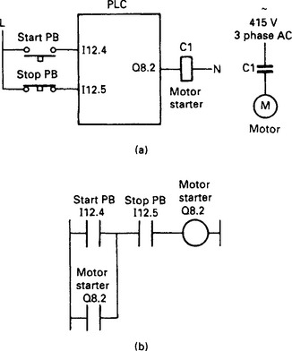
Figure 16.20 A simple motor starter in Siemens notation: (a) input/output connections; (b) the ladder diagram. Note how the stop button appears in the program
There is, however, a very important point to note about the pushbutton wiring and the program. For safety, a normally closed stop button has been used giving an input signal on I12.5 when the stop button is NOT pressed. A loss of supply to the button, or a cable fault, or dirt under the contacts will cause the signal to be lost making the program think the stop PB has been pressed causing the motor to stop. If a normally open stop PB has been used, the PLC program could easily be made to work, but a fault with the stop button or its circuit could leave the motor running with the only way of stopping it being to turn off the PLC or the motor supply.
This topic is discussed further in Section 16.7.4, but note the effect on the program in Figure 16.20. The sense of the stop button input (I12.5) inside the program is the opposite of what would be expected in a relay circuit. The input is really acting as ‘Permit to Run’ rather than ‘Stop’.
16.3.4 Logic symbols
Logic gates are widely used in digital systems (including the boards used inside PLCs). The circuits on these boards are represented by logic symbols, and these symbols can also be used to represent the operations of a PLC program. Logic symbols are used by Siemens and ABB; initially we will use Siemens notation.
The output from an AND gate, shown on Figure 16.21(a), is TRUE if (and only if) all its inputs are TRUE. The operation of the gate of Figure 16.21(a) can be represented by the table of Figure 16.21(b). In Figure 16.21(c) we have the hydraulics healthy lamp of Figure 16.19 programmed using logic symbols for a Siemens PLC. The output block, denoted by equals =, is energised when its input is true, so the lamp Q8.2 is energised (lit) when all the inputs to the AND gate are true.
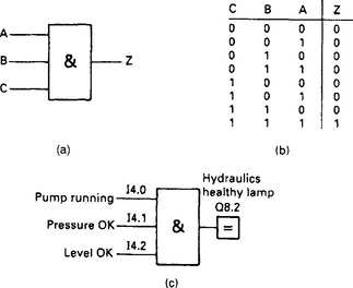
Figure 16.21 PLC programming using logic symbols: (a) an AND gate; (b) truth table for a three input AND gate; (c) the healthy lamp of Figure 16.17 using a logic symbol in Siemens notation
Often a test has to be made to say a signal is NOT true. This is denoted by a small circle ‘o’. In the earlier Figure 16.18 we illustrated the control of a hydraulic cylinder with a program which prevented the extend and retract solenoids from being energised simultaneously. This is shown programmed with logic symbols for a Siemens PLC in Figure 16.22. Note the NOT inputs on each AND gate.
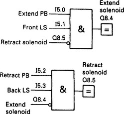
Figure 16.22 The hydraulic cylinder of Figure 16.18 in logic notation and Siemens addressing. Note the use of inverted inputs (denoted by small circles)
The output of an OR gate, Z in Figure 16.23(a), is TRUE if any of its inputs are TRUE. The inverse of a signal can be tested, as before, with a small circle ‘o’. The output Z of the gate in Figure 16.23(b) is TRUE if A is TRUE or B is FALSE or C is TRUE. In Figure 16.23(c) we have used an OR gate to add a lamp test to our hydraulic healthy lamp.

Figure 16.23 The OR Gate: (a) logic symbol; (b) OR gate with inverted input; (c) lamp test added to Figure 16.21(c)
The circuit of Figure 16.23(c) is an AND/OR combination. The ABB Master has logic combination blocks as well as the basic gates. Figure 16.24(a) is the Master block corresponding to Figure 16.23(c) (with a Master program referring to the names in its database). Similarly, for an OR/AND combination the OR/AND block of Figure 16.24(b) can be used in a Master program.
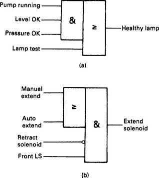
Figure 16.24 ABB Master composite gates: (a) AND/OR gate (equivalent to Figure 16.23(c)); (b) OR/AND gate
16.3.5 Statement list
A statement list is a set of instructions which superficially resemble assembly language instructions for a computer. Statement lists, available on the Siemens and Mitsubishi range, are the most flexible form of programming for the experienced user but are by no means as easy to follow as ladder diagrams or logic symbols.
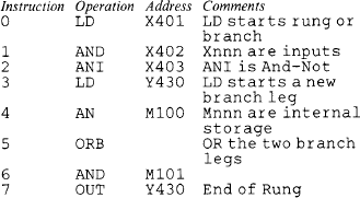
Figure 16.25 shows a simple operation in both ladder and logic formats for a Siemens PLC. The equivalent statement list would be:
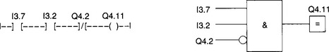
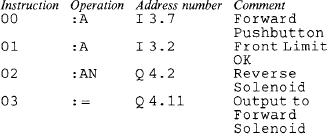
Here :A denotes AND, :AN denotes AND-NOT and : = sends the result to the output address Q4.11.
An OR operation is shown on Figure 16.26. The equivalent statement list is:
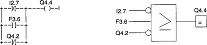

where ON denotes OR-NOT and O denotes OR.
Where a set of statements can be anomalous, brackets can be used to define the operation precisely. This is similar to the use of brackets in conventional programming where the sequence 3 + 5/2 can be written as (3 + 5)/2 = 4 or 3 + (5/2) = 5.5.
Although the latter is the default assumed by a program, the brackets do make the operation clear to the reader.
Figure 16.27 shows a typical operation, as usual in both logic and ladder diagram format. The equivalent statement list is:
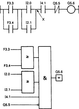
Computer programmers will recognise this as being similar to the operation of a stack with the brackets pushing data down, or lifting data up, the stack.
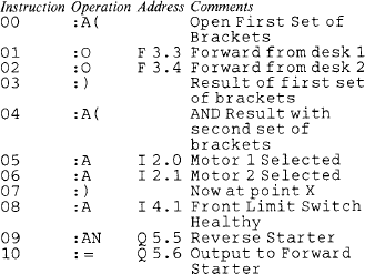
The Mitsubishi PLC also uses statement lists, although the manual recommends the designer to construct a ladder diagram first then translate it into a statement list. The PLC system shown in Figure 16.28 with Mitsubishi notation becomes the statement list:
16.3.6 Bit storage
As well as inputs and outputs, the PLC will need to hold internal signals for data such as ‘Standby Pump Running’, ‘System Healthy’, ‘Lubrication Fault’ and so on. It would be very wasteful to allocate real outputs to these signals, so all PLCs provide some form of internal bit storage. These are known variously as Auxiliary Relays, (Mitsubishi), Flags (Siemens), General Workspace (GEM-80) and Bit Storage (Allen Bradley). The notation used within the programs vary, of course, from manufacturer to manufacturer.
Mitsubishi use Mnnn with nnn representing numbers within the predefined area M100 to M377 octal. Like most small PLCs the memory layout is fixed and cannot be defined by the user. In the other, larger, PLCs we discuss, the user can define how many storage bits are needed.
The Siemens notation is F <Byte>.<Bit> (e.g. F27.06).
The GEM-80 has a variety of general work space. The commonest is called the G table, and appears in programs as G<Word>.<Bit> (e.g. G52.14). The G table is cleared when the PLC goes from a stopped state to a run state. Storage in the R table (e.g. R12.03) retains its state with the processor halted or with power removed.
Bit storage in the PLC-5 is denoted by B3/n where n denotes the signal (e.g. B3/192). The B denotes bit storage and the 3 is mandatory and arises out of the way the PLC-5 holds data in files. Bit storage is file 3; timers are file 4 (T4) and counters file 5 (C5) as we shall see later.
The ABB Master programming language does not really require internal storage bits, the function being provided by elements and connections within its database and the programming language.
Some form of memory circuit is needed in practically every PLC program. Typical examples are catching a fleeting alarm and the motor starter of the earlier Figure 16.20 where the rung remembers which button (start or stop) has been last pressed. These are known, for obvious reasons, as storage circuits.
The commonest form is shown in ladder and logic form in Figure 16.29(a). Here output C is energised when input A is energised, and stays energised until input B is de-energised.
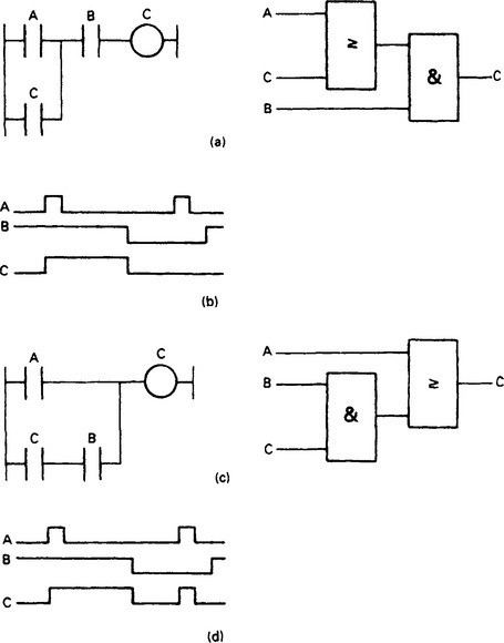
Figure 16.29 Bit storage programs: (a) commonest storage program, stop B overrides start A; (b) operation of (a), (c) Program where start A overrides stop B; (d) operation of (c)
The operation is summarised on Figure 16.29(b). As can be seen input B overrides input A, the action required of a start/stop circuit. In some circuits, however, the start is required to override the stop. We all have a typical example in our motor cars; the windscreen wipers run when we switch them on, but continue to run to the park position when we turn them off. The PLC equivalent is Figure 16.29(c), where A would be the run switch, B the park limit switch and C the wiper motor. B has again been shown energised to allow running. The operation is summarised on Figure 16.29(d).
Storage is provided in digital systems by a device called a flip flop shown on Figure 16.30(a). This has two inputs, S (for Set) and R (for Reset). The device remembers which input was last energised. If both inputs occur together, the top (S) input wins. Such a circuit is called an SR flip flop. If the device is drawn with the R input at the top, as Figure 16.30(b), the reset input will override the set input if both are present together.
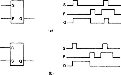
Figure 16.30 The two types of flip flop storage: (a) the SR flip flop, Set overrides R; (b) the RS flip flop, reset overrides set
The flip flop is used in logic symbol PLC programming. A motor starter using a Siemens PLC is shown in Figure 16.31. Note that the RS version has been used to ensure the stop logic overrides the run logic, and the stop signal acts as a permit to run.
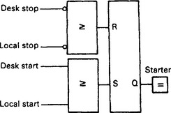
Figure 16.31 Flip flop storage is commonly preceded by logic gates. Here either stop button will reset the flip flop. Note the circles on the stop button inputs denoting inverted inputs. These are necessary because the stop buttons give a signal in the not pressed state
The ABB Master uses an almost identical symbol for the flip flop, with the addition that there are five versions. The first of these is the simple SR type shown earlier in Figure 16.30. The other versions are based on the fact that flip flops are invariably preceded by AND/OR combination of which Figure 16.31 is typical. The additional flip flops are one unit blocks consisting of a flip flop with built in AND/OR gates of user defined size. Figure 16.32 for example, is an ABB SRAO with an AND gate on the set input and an OR gate on the reset inputs. Other units are SRAA (AND/AND), SROA and SROO.

In Allen Bradley ladder diagrams, program clarity can be improved by the use of latch and unlatch outputs shown on Figure 16.33(a). These work on the same bit, setting the bit when the latch – (L) – is energised and resetting the bit when the – (U) – is energised. When both latch and unlatch are de-energised the bit holds its last state.
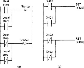
Figure 16.33 Other forms of storage: (a) the Allen Bradley latch/unlatch; (b) the Mitsubishi set/reset
The Mitsubishi F2 uses a similar idea, but calls them S and R outputs as Figure 16.33(b). This would be coded into a statement list:
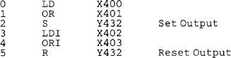
With both the Allen Bradley latch/unlatch, and the Mitsibushi set/reset, the priority goes to which ever is last in the program because of the program scan. Both the examples of Figure 16.33 correctly give priority to the stop signals.
Power failure or halting of the PLC can cause a problem with storage. When the PLC restarts should a memory bit hold the state it was in before the PLC halted, or should the memory be cleared? This is always a question of safety and convenience. A water pump in a pump house by a river 5 km from the main site should probably be allowed to restart itself if it was running before the power fail, an automatic stamping machine should almost certainly not restart.
The PLC manufacturers therefore allow the designer to choose whether a storage bit holds its state after a power fail (called retentive memory) or is cleared when the PLC is first run (called non retentive memory).
In the Allen Bradley PLC-5, this is determined by the circuit; the simple coil of Figure 16.29 is non retentive, the latch/unlatch of Figure 16.33(a) is retentive.
Other PLCs use the bit address. On a Siemens 115, flag addresses F0.0-F127.7 can be made retentive. On the Mitsubishi PLC, auxiliary relays M100-277 are non retentive, and M300-M377 are retentive. In the GEM-80, the general bit storage G Table is non retentive, a similar R Table is retentive, so a circuit similar to Figure 16.29 constructed with R3.4 as the coil and retaining contact would hold its state after a power failure.
The ABB Master uses a very structured PLC language, and forces a disciplined style on the programmer. The nature of sub elements such as memories and their behaviour when the PLC is first run is defined when the program elements are first declared.
Retentive storage can be very hazardous as plants can unexpectedly leap into life after a power fail. The designer should take care that the design does not accidentally introduce retentive features by an inadvertent selection of bit addresses.
16.3.7 Timers
Time is nearly always a part of a control system. A typical example is: ‘Lift Parking Brake, wait 0.5 seconds for brake to lift, drive to forward limit and stop drive, wait 1 second and apply parking brake’. A PLC system must therefore include timers as part of its programming language. There are many types of timer, some of which are shown on Figure 16.34
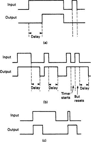
Figure 16.34 Different forms of timer: (a) the on-delay. This is the commonest timer and is often the only type available in many smaller PLCs; (b) the off-delay; (c) the fixed width pulse, often called a monostable
By far the commonest is the on-delay of Figure 16.34(a). All the other timer blocks can be built with this block and a bit of thought. A 0 to 1 transition is delayed for a preset time T, but a 1 to 0 transition is not delayed at all. An input signal shorter then T is ignored. The GEM-80 has only this type of timer, calling it a delay.
The off-delay of Figure 16.34(b) passes a 0 to 1 transition instantly but delays the 1 to 0 transition. A common use of the off-delay is to remove contact bounce or noise from an input signal. An off-delay can be obtained from an on-delay by using the inverse of the input signal and taking the inverse of the timer output signal (although the resulting program lacks some clarity).
Figure 16.34(c) is an edge triggered pulse timer, this gives a fixed width pulse for every 0–1 transition at the timer input. The PLC-5 has a Onescan pulse timer which produces a pulse lasting one (and only one) program scan. Pulses are useful for resetting counters or gating some information from one location to another.
A timer of whatever type has some values that need to be set by the user. The first of these is the basic unit of time (i.e. what units the time is measured in). Common units are 10 ms, 100 ms, 1 s, 10 s, and 100 s. The base unit does not affect the accuracy of the timer; normally the accuracy is similar to the program scan.
Next the timer duration (often called the preset) is defined. This is normally set in terms of the time base; a timer with a preset of 15 and a time base of 100 ms will last 1.5 s for example. In small PLCs this preset can only be set by the programmer, in the larger PLCs the duration can be changed from within the program itself. A delay off timer used to apply a parking brake, for example, could have different preset times dependent on whether the drive concerned is travelling at low speed or high speed.
When a timer is used there are several signals that may be available. Figure 16.35 shows the signals given for a PLC-5 delay on timer (called a TON) and a delay off timer (called a TOF).
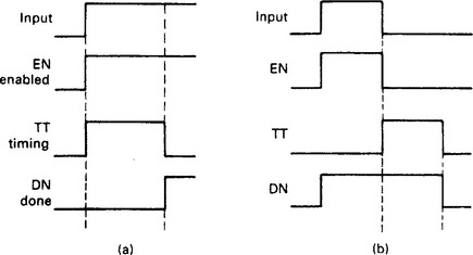
Figure 16.35 Allen Bradley timer notations: (a) EN, TT and DN for an on-delay (TON) timer; (b) EN, TT and DN for an off-delay (TOF) timer
EN (for enable) is a mimic of the timer input.
TT (for timer timing) is energised whilst the time is running.
In larger PLCs the elapsed time (often called the Accumulated Time) may be accessed by the program for use elsewhere (a program may be required to record how long a certain operation takes).
PLC manufacturers differ on how a timer is programmed. Some, such as the GEM-80, treat the timer as a delay block similar to the earlier Figure 16.34(a) with the preset being stored in a VALUE block.
Siemens use a similar idea, but have different types of timer. The PLC-5, however, uses the timer as a terminator for a rung, with the timer signals being available as contacts for use elsewhere.
Figure 16.36 shows a typical application programmed for a PLC-5 and a GEM-80 in ladder logic and a Siemens 115-U using logic symbols. The program controls a motor starter which is started and stopped via push buttons. The motor starter has an auxiliary contact which makes when the starter is energised, effectively saying the motor is running. If the drive trips because of an overload, or because an emergency stop is pressed, or there is a supply fault, the auxiliary contact signal will be lost. The contact cannot, however, be checked until 0.5 s after the starter has been energised to allow time for the contact to pull in. The program in each case checks the auxiliary contact and signals a drive fault if there is a problem. Note the difference in the way the timer is used and the fault signal is stored.
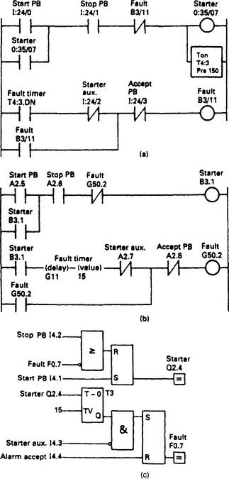
Figure 16.36 The same timer based application programmed on three different machines: (a) Allen Bradley PLC-5 TON Timer; (b) GEM-80 delay block; (c) Siemens S5 in logic notation
The accumulated time in the timers discussed so far goes back to zero each time the input goes to a zero. This is known as a non retentive timer. Most PLC timers are of this form. Occasionally it is useful to have a timer which holds its current value even though the input signal has gone. When the input occurs again the timer continues from where it stopped. This, not surprisingly, is known as a retentive timer. A separate signal must be used to reset the timer to zero. If a retentive timer is not available on a particular PLC, the same function can be provided with a counter, a topic discussed in the next section.
A typical timer can count up to 32 767 base time units (corresponding to 15 binary bits). Some older PLCs working in BCD can only count to 999. With a one second time base the maximum time will be just over 546 minutes or about 9 hours. Where longer times are needed, (or times with a resolution better than one second) timers and counters can be used together as described in the next section.
16.3.8 Counters
Counting is a fundamental part of many PLC programs. The PLC may be required to count the number of items in a batch, or record the number of times some event occurs. With large motors, for example, the number of starts have to be logged. Not surprisingly all PLCs include some form of counting element.
A counter can be represented by Figure 16.37(a), although not all PLCs will have all the facilities we will describe. There will be two numbers associated with the counter. The first is the count itself (often called the accumulated value) which will be incremented when a 0 –>1 transition is applied to the count up input, or decremented when a 0–>1 transition is applied to the count down input. The accumulated value (i.e. the count) can be reset to zero by applying a 1 to the reset input. Like the elapsed time in a timer, the value of the count can be read and used by other parts of the program.
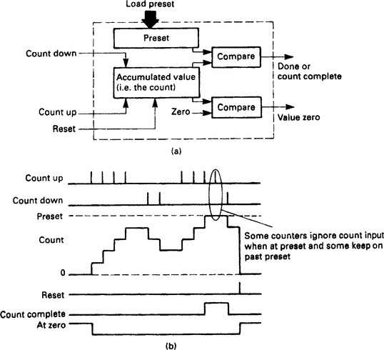
The second number is the preset which can be considered as the target for the counter. If the count value reaches the preset value, a count complete or count done signal is given. The preset can be changed by the program, a batching sequence, for example, may require the operator to change the number of items in a batch by a keypad or VDU entry. Similarly a signal zero count is sometimes available. The operation can be summarised as Figure 16.37(b).
PLC manufacturers handle counters, like timers in slightly different ways. The PLC-5 and the Mitsubishi use count up (CTU) count down (CTD) and reset (RES) as rung terminators with the count done signal (e.g. C5:4.DN) available for use as a contact.
The Siemens S5, ABB Master and the GEM-80 treat a counter as an intermediate block in a logic diagram or rung from which the required output signals can be used.
Figure 16.38 shows a simple count application performed by a PLC-5, a Siemens S5 and a GEM-80. Items passing along a conveyor are detected by a photocell and counted. When a batch is complete, the conveyor is stopped and a batch complete light is lit for the operator to remove the batch. When he does this, a restart button sets the sequence running again.
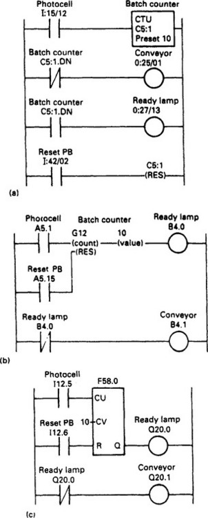
Figure 16.38 A simple batch counter programmed on three different machines: (a) Allen Bradley PLC-5; (b) GEM-80; (c) Siemens S5 in logic notation
As we saw with timers, most PLCs allow a counter to count up to 32 767. Where larger counts are needed, counters can be cascaded with the complete (or done) signal from the first counter being used to step the second counter and reset the first. Figure 16.39 is a variation on the same idea used to give a very long timer. It is shown for a PLC-5, but the same idea could be used on any PLC.
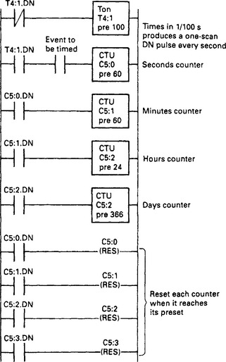
The first rung generates a free running one scan pulse with inter pulse period set by the timer period. (When the timer has not timed out, the DN signal is not present and the timer is running. When it reaches the preset, the DN signal occurs, resetting and restarting the timer.) The resulting one second pulse is counted by successive counters to give accumulated seconds/minutes/hours/days. As each counter reaches its preset it steps the next counter and resets itself.
Long duration timers built from counters are normally retentive (i.e. they hold their value when the controlling event is not present). They can be made non retentive by resetting the counters when the controlling event is not present, but this is rarely required.
16.3.9 Combinational logic
Any control system based on digital signals can be represented by Figure 16.40(a), where a system has a set of outputs Z, Y, X, W, etc. whose state is determined by inputs A, B, C, D, etc. The control scheme can operate in a combination of two basic manners.
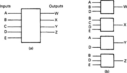
Figure 16.40 Combinational Logic: (a) top level view; (b) broken down into smaller blocks, each with one output, for programming
The simplest of these is combinational logic where the scheme can be broken down into smaller blocks as Figure 16.40(b) with one output per block, with each output state being determined solely by the corresponding input states. The loading valve for a hydraulic pump, for example, is to be energised when
The pump is running AND (Raise is selected AND top limit SW is not struck) OR (Lower is selected AND bottom limit SW is not struck)
The operation of this loading valve can be implemented with the simple ladder or logic program of Figure 16.41, but it is worth developing a standard way of producing a combinational logic program.

The first stage is to break the control system down into a series of small blocks, each with one output and several inputs. For each output we now draw up a so called truth table in which we record all the possible input states and the required output state. In Figure 16.42(a) we have an output Z controlled by four inputs A, B, C, D. There are sixteen possible input states, and Z is energised for four of these. This can be translated directly into the ladder diagram of Figure 16.42(b) or the logic circuit of Figure 16.42(c), with each rung branch and or gate corresponding to one row in the truth table. The use of a truth table method for the design of combinational logic circuits leads directly to an AND/OR arrangement called, technically, a Sum of Products (S of P) circuit.
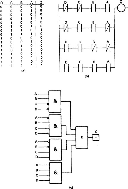
Figure 16.42 Building combinational logic from a truth table: (a) truth table; (b) Direct conversion to a ladder program. Each row in the truth table which makes Z = 1 is represented by one level on the branch; (c) Direct conversion to a logic diagram. Each row in the truth table which makes Z = 1 is represented by an AND gate. The AND gate outputs are then OR’d together
16.3.10 Event driven logic and SFCs
The states of outputs in combinational logic are determined solely by the input signals. In event driven logic (also known as a sequencer) the state of an output depends not only on the state of the inputs, but also on what was occurring previously. It is not therefore possible to draw a truth table from which the required logic can be deduced.
Consider, for example, the simple motor starter circuit of Figure 16.43(a). With neither button pressed, the motor could be running or stopped depending on what occurred last. The operation can be described by Figure 16.43(b) which is known as a state transistion diagram, (often shortened to state diagram).

Figure 16.43 A simple state transition diagram; (a) A motor starter; (b) State transition diagram. Note that with no buttons pressed the system can be in either state
The square boxes are the states the system can be in; the motor can be running or stopped, and the arrows are the transitions that cause the system to change states. If the motor is running, pressing the stop button will cause the motor to stop. A bar above a signal (e.g. above stop PB OK) means signal not present; note the wiring of the stop PB and the signal sense. It is a useful convention to label states with numbers and transitions with letters.
State transition diagrams can be constructed from storage elements, with one less storage element than there are states, and the one default state being inferred by the absence of others. It therefore requires just one storage element (latch, SR flip flop or whatever) to implement the motor starter of Figure 16.43.
Figure 16.44 is a more complex example (based on a real silo). A preset weight of material is fed into a weigh hopper ready for the next discharge, which is initiated by a Discharge pushbutton. A hood then lowers (to reduce dust emissions) and the material discharges. After the discharge, the hood retracts and the weighhopper re-fills. An abort pushbutton stops a discharge, and a feed permit switch stops the feed.

Figure 16.44 A more complex state transition diagram for a real plant: (a) physical layout; (b) state transition diagram; (c) output table
There are two fault conditions; failure to get the batch weight in a given time (probably caused by material jamming in the feeder) and failure to get zero weight from the discharge (again in a given time and again probably caused by a material jam). Both of these trip the system from automatic to manual operation to allow the cause of the fault to be determined.
We can now draw the state diagram of Figure 16.44(b). The default state is the state that the system will enter from manual, and care needs to be taken in its selection. Here feed is the sensible choice; if the hopper if already full the system will immediately pass to state 1 (ready), if not, the hopper will be filled. The choice of any other state as default could lead to a wasted cycle through all the states with no material in the weigh hopper.
We can now construct a table linking the outputs to the states. This is straightforward and is given on Figure 16.44(c).
The next stage is to translate this state diagram into a PLC program. The programming method relies very much on the idea of the program scan, described earlier in Section 16.2.4. By breaking down the program for our state diagram into four areas as Figure 16.45 we can control the order in which each stage operates. The actual layout is not critical, but it is essential for transitions and states to be kept separate and not mixed.

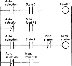
Automatic/manual selection comes first, this is achieved with the simple rung of Figure 16.46. Automatic mode is only allowed if there are no faults and the hood is raised.

Next come the transitions, some of which are shown on Figure 16.47. These are straightforward and need little comment. Note that the first contact in each rung is a state, so inputs are only examined at the correct point in a sequence.
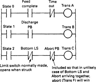
Some of the states themselves are given in Figure 16.48. With the exception of state 0, simple latches have been used throughout for the states and the auto/man selection so that after a power failure the system will resume in manual mode. Note that these are set and reset by the transitions.
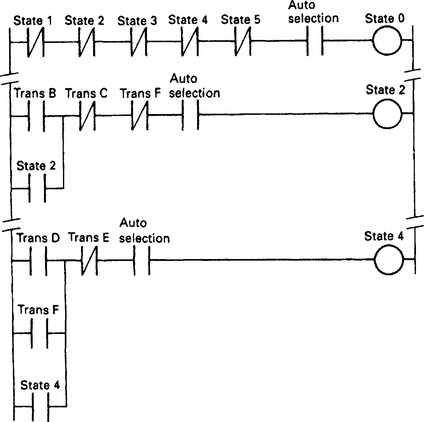
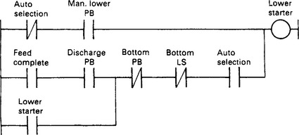
Finally we have the outputs themselves on Figure 16.49. An output is energised during the corresponding state(s) in automatic or from the manual maintenance push button in manual.
The state diagram technique is very powerful, but it can lead to confusion if the basic philosophy is not understood. The often quoted argument is it takes more rungs or logic elements than a direct approach programmed around the outputs.
This is true, but programming around the outputs can lead to very twisted and difficult to understand programs. Figure 16.50 is one rung roughly corresponding to state 2 of our state diagram. It mixes manual and automatic operation and its action is by no means clear (known colloquially as Spaghetti programming). Problems can arise where transitions go against the program scan as transition E on the earlier Figure 16.44(b). If care is not taken, a sequence based purely on outputs can easily end up doing two things at once, or nothing at all because of the way the program scan operates. Modifications are also tricky with a direct approach, but simple with a state diagram.
State diagrams are being formalised by the International Electrotechnical Commission and the British Standards Institute, and already exist with the French Standard Grafset. These are basically identical to the approach outlined above, but introduce the idea of parallel routes which can be operated at the same time. Figure 16.51(a) is called a divergence, state 0 can lead to state 1 for condition s OR to state 2 for condition t with transitions s and t mutually exclusive. This is the form of the state diagrams described so far.
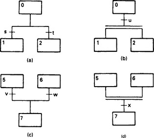
Figure 16.51 Grafset symbols: (a) divergence; (b) simultaneous divergence; (c) convergence (d) simultaneous convergence
Figure 16.51(b) is a simultaneous divergence, where state 0 will lead to state 1 AND state 2 simultaneously for transition u. States 1 and 2 can now run further sequences in parallel.
Figure 16.51(c) again corresponds to the state diagrams described earlier, and is known as a convergence. The sequence can go from state 5 to state 7 if transition v is true OR from state 6 to state 7 if transition w is true.
Figure 16.51(d) is called a simultaneous convergence (note again the double horizontal line) state 7 will be entered if the left-hand branch is in state 5 AND the right-hand branch is in state 6 AND transition x is true.
The state diagram is so powerful that most medium size PLCs include it in their programming language in one form or another. Telemecanique give it the name Grafcet (with a ‘c’), others use the name Sequential Function Chart (SFC) (Allen Bradley) or Function Block (Siemens). We will return to these in the next chapter.
Even the simple Mitsubishi F2 supports state diagrams with its STL (Stepladder) instruction. These have the prefix S and can range from S600 to S647. They have the characteristic that when one or more are set, any others energised are automatically reset. A RET instruction ends the sequence. The state diagram of Figure 16.52(a) thus becomes the ladder diagram of Figure 16.52(b).

Figure 16.52 State diagrams on the Mitsubishi F2: (a) state diagram; (b) part of the ladder diagram corresponding to (a)
Where there are no branches and the sequence is a simple ring (operating rather like a uniselector) a sequence can be driven by a counter which selects the required step. The counter is stepped when the transitions for the current step are met. The GEM-80 has a SEQR (sequence) instruction which acts as a sixteen step uniselector.
16.3.11 IEC 1131
We have seen that PLCs can be programmed in several different ways. In recent years the International Electrotechnical Commission (IEC) have been working towards defining standard architectures and programming methods for PLCs. The result is IEC 1131, a standardised approach which will help at the specification stage and assist the final user who will not have to undergo a mind-shift when moving between different machines.
The earliest, and probably still the commonest, programming method described is the Ladder Diagram (or LD in IEC 1131).
Function Block Diagrams (FBDs) use logic gates (AND/OR etc.) for digital signals and numeric function blocks (arithmetic, filters, controllers, etc.) for numeric signals. FBDs are similar to PLC programs for the ABB Master and Siemens SIMATIC families. There is a slight tendency for digital programming to be done in LD, and analog programming in FBD.
Many control systems are built around state transition diagrams, and IEC 1131-3 calls these Sequential Function Charts (SFCs). The standard is based on the French Grafcet standard shown earlier on Figure 16.51.
Finally are text based languages. Structured Text (ST) is a structured high level language with similarities to Pascal and C. Instruction List (IL) contains simple mnemonics such as LD, AND, ADD etc. IL is very close to the programming method used on small PLCs where the user draws a program up in ladder form on paper, then enters it as a series of simple instructions.
Figure 16.53 illustrates all of these programming methods.

A given project does not have to stick with one method, they can be intermixed. A top level, for example, could be an SFC, with the states and transitions written in ladder rungs or function blocks as appropriate.
It will be interesting to see the effect of IEC 1131-3. Most attempts at standardisation fail for reasons of national and commercial pride. MAP, and latterly fieldbus, have all had problems in gaining wide acceptance. A standard will be useful at the design stage, and could be accepted by the end user if programming terminals presented a common face regardless of the connected machine.
16.4 Numerics
So far we have been primarily discussing single bit operations. Numbers are also often part of a control scheme; a PLC might need to calculate a production rate in units per hour averaged over a day, or give the amount of liquid in a storage tank. Such operations require the ability to handle numeric data.
16.4.2 Numeric representations
Most PLCs work with a 16 bit word, allowing a positive number in the range 0 to +65 535 to be represented, or a signed (positive or negative) number in the range −32 768 to +32767. In the latter case, known as two’s complement, the most significant bit represents the sign, being 1 for negative numbers and 0 for positive numbers.
Numbers such as these are known as integers, and can only represent whole numbers in the above range. Where larger whole numbers are required, two sixteen words can be used allowing a range −2147483 648 to +2147483 647. This type of integer is available in the ABB Master (where it is known as a long integer) and the 135-U and 155-U in the Siemens family (where the term double word integer is used).
Where decimal fractions are needed (to deal with a temperature of 45.6°C for example) a number form similar to that found on a calculator may be used. These are known as real or floating point numbers, and generally consist of two sixteen bit words which contain the mantissa (the numerical portion) and the exponent. In base ten, for example, the number 74057 would have a mantissa of 7.4057 and an exponent of 4 representing 104. PLCs, of course, work in binary and represent mantissa and exponent in two’s complement form.
Real numbers are very useful but their limitations should be clearly understood. There are two common problems. The first occurs when large numbers and small numbers are used together. Suppose we had a system operating to base ten with four significant figures, and we wish to add 857 800 (stored as 8.578E5) and 96 (stored as 9.600E1). Because the smaller number is outside the range (four significant figures) of the larger, it will be ignored giving the result 857 800 + 96 = 857 800.
The second problem occurs when tests for equality are made on real numbers. The conversion of decimal numbers to binary numbers can only be made to the resolution of the floating point format. If real numbers must be used for comparison, a simple equates (=) is very risky. The composites > =, (greater than or equals), and < =, (less than or equals), are safer, but it is generally better practise to use integers for tests if at all possible.
The final representation, BCD for Binary Coded Decimal, is used for connection to outside world devices such as digital displays or thumbwheel switches. Such devices are arranged in a decimal format, with 4 binary bits per decade, for example1 0 0 1 0 1 0 1
can be interpreted in BCD as 95.
This representation is wasteful, as six ‘numbers’ are not used per four bits (10 to 15 inclusive). It is, however, a convenient form to use with external wiring. Most PLCs therefore have instructions which convert BCD to the internal binary format of the PLC, and binary back to BCD.
The types of numbers available in each PLC range vary considerably according to the model (and obviously the price). The Mitsubishi F2, for example, purely allows movement, comparison and output of numerical data from counters or timers, making it essentially a bit operation machine.
In the Siemens range, the popular 115-U uses only 16 bit integer numbers but the next model in the range, the 135-U, can handle 16 bit and 32 bit integers and floating point numbers. A similar spread of capabilities will be found amongst the Allen Bradley, GEM-80 and ABB families.
16.4.3 Data movement
Numbers are often moved from one location to another; a timer preset may be required to be changed according to plant conditions, a counter value may need to be sent to an output card for indication on a digital display or the result of some calculations may be used in another part of a program.
The Allen Bradley PLC-5 uses one rung per move operation, and is possibly the simplest to explain first. Its simplicity of one rung per operation is continued in all the arithmetic functions we shall consider, but it can lead to more rungs being used for a given operation than in other machines.
Figure 16.54(a) shows the form of the rung. It starts with some binary conditions; if these are all made the output MOV (for MOVE) is obeyed, transferring data from the source to the destination. The source and destination can be any location where numerical data can occur, for example
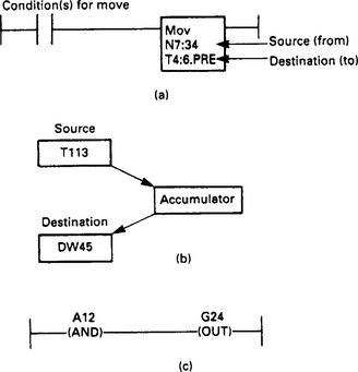
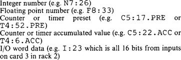
If data is transferred between integer and floating point forms, the conversion is performed automatically however care must be taken transferring floating point numbers to integers as an error can occur if the floating point number is outside the integer range. Finally, as a source only, a constant (such as 3, 17 or 4057) can be used.
The example of Figure 16.54(a) thus moves the number held in N7:34 to the preset of timer T4:6 when the rung conditions are met.
Siemens and GEC use a slightly different approach which leads to more compact programs. Both treat a data movement as two separate instructions via a separate accumulator (a single word storage location). Siemens use the instructions load to move data from a source to the accumulator, and transfer to move data from the accumulator to the destination as Figure 16.54(b). The data can come from (or go to) any data storage area, some of which are
| IW | a 16 bit input word |
| QW | a 16 bit output word |
| T | a timer word |
| C | a counter word |
| DW | a 16 bit data storage word |
Figure 16.54(b) would thus be programmed as
![]()
The use of the accumulator is not obvious in the GEM-80. The −<AND>- instruction puts the binary number from the specified location (again internal storage or I/O) into the rung, and the −<OUT>− instruction puts the value from the rung to the specified address. In Figure 16.54(c) the (binary) value from 16 bit input word A12 is placed into 16 bit storage word G24.
BCD/binary conversion is available with −<BCDIN>− and −<BCDOUT>− instructions, the direction of the conversion being obvious.
In the ABB Master, the points between which data is to be transferred are simply linked on the logic diagram.
16.4.4 Data comparison
Numerical values often need to be compared in PLC programs; typical examples are a batch counter saying the required number of items have been delivered, or alarm circuits indicating, say, a temperature has gone above some safety level.
These comparisons are performed by elements which have the generalised form of Figure 16.55, with two numerical inputs corresponding to the values to be compared, and a binary (on/off) output which is true if the specified condition is met.
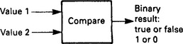
Many comparisons are possible; most PLCs provide
| A Greater Than B | (A>B) |
| A Greater Than or Equal to B | (A>=B) |
| A Equals B | (A=B) |
| A Less Than or Equal to B | (A<=B) |
| A Less Than B | (A<B) |
where A and B are numerical data. With real (floating point) numbers the equal test should be avoided for the reasons given in the previous section. There are many other possible comparisons; a PLC-5, for example has a limit instruction which tests for A lying between B and C and the GEM and Siemens have a not equal test.
Figure 16.56 shows the setting and resetting of an alarm flag B3/21 (for a PLC-5 ladder diagram) and F21/02 (for Siemens logic symbols). The alarm bit is set if temperature (read from an analog input card in format NN.N°C and held in N7:15 in the PLC-5 or DW42 in the Siemens 115-U) goes above 50.0 °C. Once set, the alarm is stored until the temperature goes below 40.0 °C.
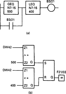
16.4.5 Arithmetical operations
Numerical data implies the ability to do arithmetical operations, and all PLCs we are considering (apart from the simple F2) provide the ability to do at least four function maths (add, subtract, multiply and divide).
In Section 16.4.2 we discussed integer and floating point numbers. Care needs to be taken with integer operations. The range of a 16 bit two’s complement number is −32 768 to +32 767. If an arithmetical operation goes outside this range, the number will overspill, for example

which is not quite the expected result. The PLCs have an overspill flag which can be examined and used to flag an alarm, or set the result to, say, zero with a move instruction. Similar precautions need to be taken with subtraction and multiplication (the latter being particularly vulnerable to giving an overspill; for example 200 × 200 = 40 000, well over-range.)
Even greater care needs to be taken with division. A fault condition on external plant or a PLC input card or a programming error can lead to a divide by zero error. This will stop many PLCs dead in their tracks with a ‘Program Fault’. It is therefore good practice to proceed any vulnerable divide instruction with a limit check to ensure it will only be obeyed when a sensible result is obtained.
Each PLC manufacturer handles arithmetic in a slightly different way with varying degrees of ease and readability. None are as simple as a high level language such as BASIC or Pascal, and the facilities are generally limited to four function maths plus square root in all bar the most expensive machines.
A PLC-5 uses maths blocks such as ADD, SUB, MULT, DIV, giving a simple, if somewhat lengthy, program. Figure 16.57 shows how a simple calculation could be performed for a self correcting length cutting program. More powerful PLC-5s (such as the 5–40) have a block compute instruction (CPT) which allows a mathematical expression to be evaluated in a single instruction.
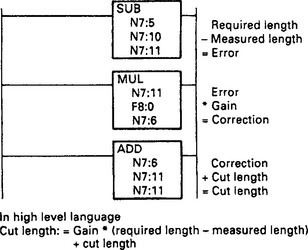
The 115-U only evaluates arithmetic instruction in STL (statement list) format. It will be remembered from our discussion of the accumulator that the load, (L) and transfer (T) instructions use an internal accumulator. There are, in fact, two accumulators, and a load instruction moves the contents of accumulator 1 to accumulator 2 then moves the contents of the source to accumulator 1, shown in Figure 16.58(a). An arithmetic instruction (add, subtract, etc.) works on the contents of both accumulators. Figure 16.58(b), thus adds two numbers and transfers the result to storage.
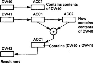
The Siemens equivalent of Figure 16.57 would be
| L DW30 | (required length) |
| L DW31 | (measured length) |
| SUB | (leaving error in Acc 1) |
| L DW32 | (gain) |
| MULT | (leaving correction) |
| L DW40 | (the old cut length) |
| ADD | (add change to give new length) |
| T DW40 | (put back to store) |
The most understandable form of representation is possibly the GEM-80 ladder and the ABB Master formats shown in Figure 16.59(a) and (b) respectively.
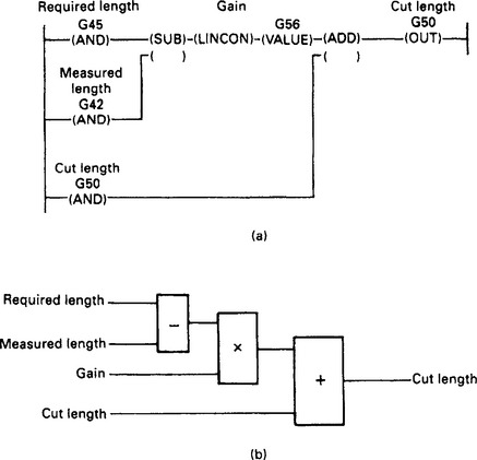
Figure 16.59 The same mathematical function in a GEM-80 and ABB Master: (a) GEM-80 program. LINCON is an arithmetic function used to avoid truncation errors with integer arithmetic; (b) ABB master program using function blocks. Variables are accessed by database names
All maths operations, particularly those involving floating point numbers, are time consuming, and it is good programming practice to only obey instructions when they are needed, and not waste time repetitively obeying them on every PLC scan.
16.4.6 Analog signals
So far we have considered signals that are essentially digital (on/off) in nature plus simple numerical data from timers and counters. Often, though, a PLC will be required to measure, or control, plant signals which can assume any value in some predetermined range. Typical signals of this type are temperatures, flows, pressure, speeds etc. These are known as analog signals. In a similar way a PLC may have to produce analog output signal to drive meters and proportional valves or provide a speed reference for a motor drive controller.
To meet these requirements a PLC needs analog input and output cards. These have somewhat different characteristics to the simple digital cards we have discussed so far. This section considers analog signals and the way they are handled.
An analog input card converts a continuously varying analog signal to a digital form that can be used inside a PLC program. The analog signal is generally represented initially, at least, as an integer number.
This analog to digital conversion (usually known by the initials ADC) is inherently accompanied by a loss of resolution which depends on the number of bits used. An 8 bit byte for example, can represent an integer in the range 0–255. If this was used to represent an analog signal measuring a flow with a span (range) from 0–1800 1/min, one bit will represent approximately 71/min (given by 1800/255). Any control strategy in the program based on finer resolution is meaningless (and particular care should be taken with comparisons, as some values can never be obtained; a flow of 138 1/min, for example, would never be given by our 8 bit system, it would jump from 134 1/min to 141 1/min. Comparisons should therefore always be based on (greater than or equal to) or (less than or equal to)).
A commoner resolution is 12 bits. This gives a representation as an integer from 0–4095. With our flow of 0–1800 1/min, one bit would represent just under 0.5 1/min (1800/4095 = 0.44).
This ‘coarseness’ is not the problem it might at first appear. Although an analog transducer can give any value in its span, it will have inherent errors. Many first line transducers are only 2% accurate. If our flow transducer had 2% accuracy, its measurement could be in error by 36 1/min. Alongside this error, the 7 1/min resolution from an eight bit card is probably quite reasonable.
It is therefore useful to think of the resolution in terms of an error which is to be added to the error from the transducer itself
| No of bits | Range | Error |
| 8 | 0-255 | 0.5% |
| 10 | 0-1023 | 0.1% |
| 12 | 0-4095 | 0.025% |
Few industrial transducers have an accuracy better than 0.1%, and a 12 bit conversion will add little error in most applications.
The conversion from an analog signal to a digital representation is not instantaneous. Typically signals are read ten times per second. An analog input card thus takes regular ‘snapshots’ of each analog signal. In Figure 16.60(a) this causes no problems, in Figure 16.60(b) information is starting to be lost and in Figure 16.60(c) a totally false view of the signal is being given. This latter effect is known as ‘aliasing’.
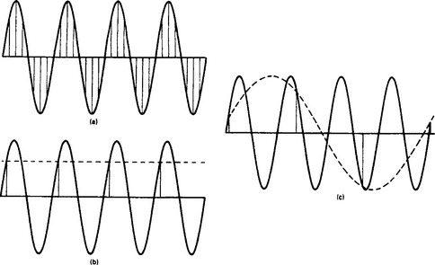
It is therefore very important to have a sufficiently fast conversion time. Every analog signal will have a maximum frequency at which it can change, and can be represented by a gain/frequency plot as Figure 16.61 from which the bandwidth and the critical frequency fc can be observed. To get a true series of ‘snapshots’ we must sample the signal at least twice the rate of fc. If a certain analog signal has a maximum frequency of 2 Hz, we must at least sample it at 4 Hz, or once every 250 ms. This, somewhat simplified, is known as Shannon’s sampling theorem. In real systems, fc is rarely known precisely and a scan rate of 4 fc to 10 fc is normally chosen to give a reasonable safety margin. For our 2 Hz signal, an 8 Hz sampling rate or 12.5 ms conversion time, would be needed. It is good practice to pass the signal through a low pass filter before the ADC to ensure frequencies above fc are removed. This is known as an anti-aliasing filter.
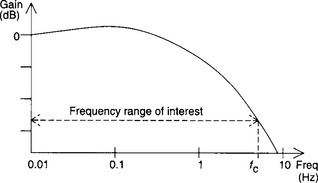
Surprisingly this rarely gives problems. Practical industrial systems, dealing with real plant signals concerned with materials with significant mass, rarely have bandwidths greater than 0.5 Hz, and any frequency higher than this can be considered to be extraneous noise and filtered out. Temperature loops, for example, can often be sampled as slowly as once every few minutes without introducing any errors.
A typical analog input card can read eight 12 bit signals, each ranging from 0–4095 in their ‘raw’ form. Generally these will need to be accessed via the PLC program and converted to engineering units such as °C, or psi, or 1/min.
A common method of handling these signals, is shown in Figure 16.62. A block of storage locations in the PLC store is directly associated with the analog input card. The card ‘free runs’, writing digitised values into the store from where they can be read by the rest of the program. In Siemens PLCs with fixed slot addressing, for example, the store addresses are determined directly by the analog card position in the rack; a card in slot 2 of the first rack will write its values to a block of stores starting at location 192.
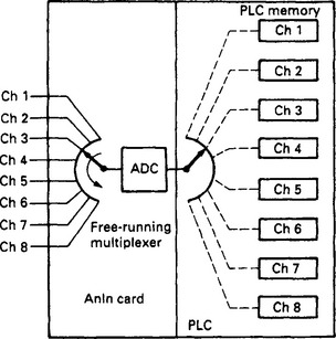
Conversion from a raw 12 bit signal to engineering units can have subtle traps for the unwary. In theory the conversion is simple. If N is the raw signal, HR the high range signal (corresponding to 4095) and LR the low range (corresponding to zero) then the measured value, Mv is simply
If the calculation is done with real (floating point) numbers there should be no problem, and Equation 16.1 can be used directly.
If, however, integer numbers have to be used, great care must be taken. If the multiplication N × (HR − LR) is performed first, arithmetic overspill is likely unless 32 bit results can be accommodated. If the division N/4095 is performed first, the equation will not work as N is always less than 4095 giving an integer result of zero (and an Mv of LR). Wherever possible real numbers should be used if Equation 16.1 has to be performed.
To avoid this problem, the different manufacturers have devised methods to read analog input signals. In the ABB Master for example, the database for each signal defines HR, LR, the sample rate and a name by which the signal will be referred to in the program. There are, obviously, detail differences, so by way of example we will look at the way analog signals are read by an Allen Bradley PLC-5.
The Allen Bradley PLC-5 reads analog signals with an analog input card (1771-IFE) which can in its simplest form, read 8 analog inputs. The PLC communicates with the card via instructions called block transfers which transfer data to (or from) a block of store locations. Data transfers from the PLC to a card are called block transfer writes (BTW) and, not surprisingly, transfers from a card to the store are block transfer reads (BTR). For each type of instruction, somewhat simplified, the programmer states:
(a) The direction of transfer (BTW or BTR).
(b) The card address (rack, slot and slot half, left or right).
(c) The store location start address where the data is to be received.
The analog input card uses both BTW and BTR instructions, the BTW being used once, after power up, to configure the module and the BTRs subsequently to read the data as summarised in Figure 16.63.
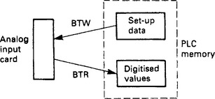
The post power up BTW sets how the module is to behave; whether it gives data in binary or BCD and the minimum and maximum values for the input range (HR and LR in Equation 16.1) on each channel. The card uses these to return readings in engineering units (in 12 bit binary integer or two’s complement format or 12 bit BCD).
Once set up, values can be read at the required time intervals with a BTR. This gives signal values in the specified store locations along with over-range and similar alarms. The values can then be used elsewhere in the program.
PLCs are often required to provide analog output signals. Like analog inputs, these signals have standard voltage ranges of 1–5 V or 0–10 V or the current range of 4–20 mA.
A typical analog output card, for example, is the Allen Bradley 1771-OFE which has four output channels, each turning a 12 bit (0–4095) digital signal into an analog output. Isolation amplifiers are used on the outputs to reduce the effects of noise and allow the signals to connect into external devices fed from different electrical supplies. The digital signals come from storage locations inside the PLC as shown on Figure 16.64. This conversion is known as Digital to Analog conversion, or DAC.
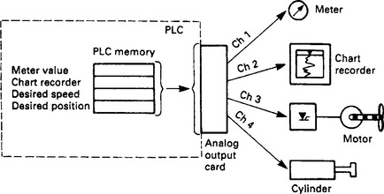
For best resolution the PLC should use the full 0–4095 range, but this is frequently impossible. If the PLC, for example, is setting the speed range of a motor from 0–1350 rpm, it will need to convert 0–1350 into the range 4–20 mA. Equation 16.1 can be re-arranged as
where X is the value passed to the DAC (in the range 0–4095). N is the output number from the PLC in engineering units, and HR/LR are the high and low range values. As before, great care must be taken with Equation 16.2 to avoid overspill or loss of resolution.
The PLC-5 communicates with the 1771-OFE with the BTW instruction described previously. The programmer sets up a block of twelve words, the first four of which contain the values, and the balance the set up data such as HR and LR. The block of data is then written to the card with a BTW. Figure 16.65 shows a typical example where an analog speed reference can be raised or lowered by operator controlled pushbuttons. Note the use of greater than (GTR) and less than (LES) instructions to confine the counter value within the allowed range of 0–1350 rpm.
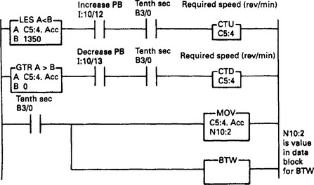
Ranging as above allows engineering units to be used inside the program, the counter in Figure 16.65, for example, holds the required speed directly in rpm, but this is accompanied by a loss of resolution as explained earlier. For the range 0–1350 rpm, we have a resolution of about 0.1%, compared with the theoretical 0.025% resolution available from the card.
There are other operations that can be performed on analog signals. A typical list, for the GEM-80, is
| SQRT | Square root, mainly used with signals from orifice plates. |
| LINCON | Performs X*(A/B) + C with limiting. |
| FGEN | Multipoint straight-line function generator used for linearisation as Figure 16.66(a). |
| LIMIT | Performs limiting of signals as shown on Figure 16.66(b). |
| RAMP | Rate limiting (with different rise and fall rates). |
| DEDBAND | Deadband functions as Figure 16.66(c). |
| Useful for preventing ‘dither’ in closed loop control when PV and SP are close. | |
| ANALAG | First Order lag. Used for filtering. |
A simple first order filter can be produced by any PLC which supports floating point numbers using the procedure shown on Figure 16.67(d). This procedure uses just three rungs or three function blocks and is obeyed for one program scan at regular time intervals Δt. Vi is the raw input signal and Vf is the filtered output signal, Vf(n-1) is the filtered value obtained on the previous execution Δt seconds ago. The error between Vi and Vf(n-1) is calculated (Ve) then multiplied by a gain K to give a change Vc. This is added to Vf(n-1) to give the new filtered value Vf. Figure 16.67(b) shows the response for a step change in V, with K set at 0.25. At each execution of the routine Vf moves 25% of the difference between V, and Vf(n-1). The gain, K, determines the apparent time constant and must be in the range 0 < K < 1. The gain K should be set to Δt/T where T is the required time constant.
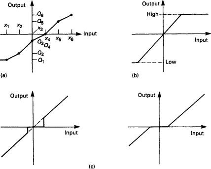
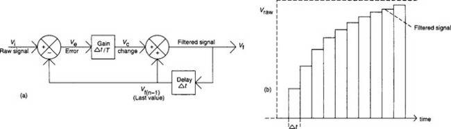
16.4.7 Closed loop control
A closed loop system based on PLCs will be similar to Figure 16.68. The plant variable, Pv, is read by an analog input card, and the output OP provided by analog output cards. The setpoint, SP, is provided by the operator or by some program sequence. The PID algorithm is then provided by the program. Chapter 13 gives more detail on the theory of closed loop control and an explanation of the PID algorithm.

It is possible to write PID algorithms with four function (+ − */) mathematics, but it needs great care. The program scan time must be known for the integral and derivative routines, and protection against output actuator saturation must be built in to overcome an effect called integral wind-up.
PLCs, are becoming increasingly powerful, and most medium range PLCs now provide a three term PID function in their instruction set. Figure 16.69 shows a ratio temperature control program written for an Allen Bradley PLC-5 processor.
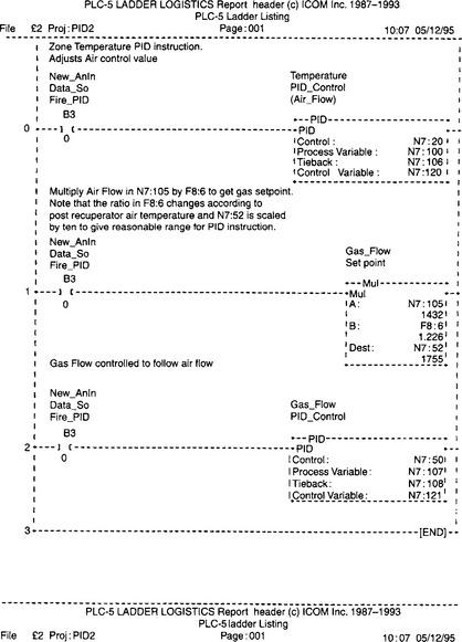
These three rungs are controlling the temperature in a furnace, with the temperature PID block controlling the air valve. The air flow is measured, multiplied by the required ratio and used as the setpoint for the gas PID block.
The control blocks in each PID instruction hold the data and working areas for the PID function; things like auto/man status and the sum for the integral action. The setpoint is written directly into the third word of the control block. The process variable is the feedback signal from the variable being controlled, usually obtained from an analog input card. Settings for gain, Ti and Td are also contained in the control block data.
A three term control algorithm can suffer from integral wind-up in saturation or manual operation. The tieback variable is used to give the current value corresponding to the driven actuator output (possibly after auto/manual changeover) and is used to prevent wind-up and to give bumpless transfer. The control variable is the signal from the PID algorithm, usually sent to an analog output card via auto/manual changeover logic.
The three rungs of Figure 16.69 mask, to some extent, the work that must be done elsewhere in the program. Data from the outside world must be obtained with analog input cards, and the controller output(s) must be written to the actuators with analog output cards. The timing of these reads and writes must be regular and linked to the PID instructions.
Auto/manual changeover logic will also be required, linked into the PID instructions with the tieback variable and the auto/man status flag (which makes the integral term track the tieback in manual).
The operator will also require a link to the control, so pushbuttons, displays and alarms must be provided. All of this is in addition to the basic PID control.
16.4.8 Intelligent modules
We have so far considered analog input and output modules, which are semi-intelligent (compared to ‘dumb’ digital input and output cards). These are examples of a more general range of intelligent modules which most manufacturers offer to simplify the designers task.
A typical example is a high speed counter. We saw earlier in Section 16.2.4 that the scan time limits the maximum count rate of a PLC to about 10 Hz. High speed counter cards are available for use where higher count speeds are needed, or the program scan time introduces an unacceptable random error.
In these, the card contains a bi-directional counter which can be directly driven by a pulse encoder. The counter value can be loaded from the PLC, and read back when needed. The PLC can also download a preset value, allowing the counter card to directly drive outputs according to the relationship between the count and the preset.
Other common intelligent modules are bar code readers (for stock tracking), stepper motor controllers (for position control systems) and vision modules (for quality control applications).
16.5 Distributed systems and fieldbus
For a true distributed control system we need a method where several PLCs or computers can be linked together to allow communication to freely take place between any member of the system.
To achieve this we need to establish a connection topology, some way of sharing the common network that prevents time wasting contention and an address system that allows messages to be sent from one member to another. Such systems are known as Local Area Networks (LAN) or Wide Area Networks (WAN) dependent on the size of the area and the number of stations.
16.5.2 Transmission lines
Any network will be based, to some extent, on cable, and at the high speeds used there are aspects of transmission line theory that need to be considered. Consider the simple circuit of Figure 16.70(a). At the instance that the switch closes, the source voltage does not know the value of the load at the far end of the line. The initial current step, i, is therefore determined not by the load, but by the characteristics of the cable (dependent on the inductance and capacitance per unit length). A line therefore has a characteristic impedance, typically 75 Ω or 50 Ω for coax, and 120 to 150 Ω for biaxial or screened twisted pair. The initial current step will therefore be V/Z where Z is the characteristic impedance.
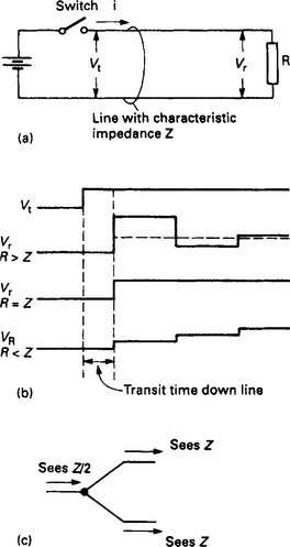
Figure 16.70 Transmission lines and the characteristic impedance: (a) a transmission line; (b) the effect of the terminating resistor; (c) The effect of a ‘T’ in the line
After a finite time, this current step reaches the load R, and produces a voltage step i × R. If R is not the same as Z, this voltage step will not be the same as V, and a reflection will result. Typical results are shown on Figure 16.70(b).
This effect occurs on all cables and is normally of no concern as the reflections only persist for a short time. If, however, the propagation delay down the line is similar to the maximum frequency rate of the signal, the reflections can cause problems. It follows that a transmission line should be terminated by a resistance equal to the characteristic impedance of the line. Normally, devices for connecting onto a transmission line have a high input impedance to allow them to tap in anywhere, with terminating resistors being used at the ends of the line.
A side effect of this is that T connections, or spurs, are not allowed (unless the length of the spur is short). In Figure 16.70(c) a T has been formed. To the signal, coming from the left, the two legs appear in parallel giving an apparent impedance of Z/2 and a reflection.
16.5.3 Network topologies
From the previous section it should be apparent that any network can sensibly only be based on a ring (which needs no terminating resistors) or a line (with a terminating resistor at each end). Figure 16.71 is a master/slave system where a common master wishes to receive or send data from/to slave devices, but the slaves never wish to talk to each other. All the slaves have addresses, which allows the master to issue commands such as ‘Station 3; give me the value of analogue input 4’ or ‘Station 14; your setpoint is 751.2’. Such systems are often based on RS422 to provide improved noise immunity and allow longer lengths of line.

The Star network of Figure 16.72 is again based on a master with a point to point link to individual stations. This arrangement is commonly used for high level computer systems. Communication control is performed by the master station. Station to station communication is possible via, and with the co-operation of, the master.
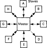
In Figure 16.73 all the stations have been connected in a ring. There is no master, and all stations can talk to any other station and all have equal right of access. The term peer to peer link is often used for this arrangement. With Figures 16.71 and 16.72 control was firmly in the hands of the master. With the ring, some technique is needed to avoid clashes when two stations wish to use the line at the same time. We will discuss this in the following section.
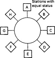
Figure 16.74 is probably the commonest type of network used by PLCs. It is a single line with terminating resistors and, like the ring, is a peer to peer link where all stations have equal standing.
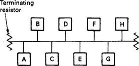
16.5.4 Network sharing
A peer to peer link allows many stations to use the same network. Inevitably two stations will want to communicate at the same time. If no precautions are taken, the result will be chaos. Various methods are used to govern access to the network.
One idea is to allocate time slots into which each station can put its messages. This is known as Time Division Multiplexing, or TDM. Whilst it prevents clashes, it can be inefficient as a station will have to wait for its time slot even if no other station has a message to send. To some extent a mismatch between the frequency of messages from different stations can be overcome by giving more slots to hardworking stations. This is sometimes known as Statistical TDM.
The empty time slot of Figure 16.75 uses a packet which continuously circulates around the ring. When a station wishes to send a message it waits for the empty slot to come round, when it adds its message. In Figure 16.75, station A wishes to send a message to station D. It waits until the empty packet comes round. Then it puts its message onto the network along with the destination address D. Stations B and C pass the message but ignore it because it is not for their address. Station D matches the address, reads the contents (and appends that it has received the message). Stations E-H ignore it, but pass it on. Station A receives the message back again, sees the acknowledgement and removes its message leaving the empty packet circulating the ring again. A similar idea is a token passing, where a ‘Permit to Send’ token circulates round the network. A station can only transmit when it is in possession of the token, which is released when the acknowledgement that the message arrived is received.
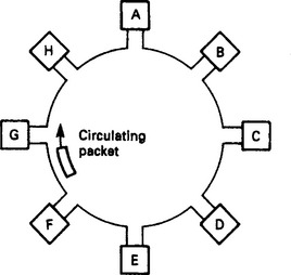
Bus systems usually employ a method where a station wishing to send a message listens to the network to see if it is in use. If it is, the station waits. If the network is free, the station sends its message (thereby locking out any other station until the message ends). This is known as Carrier Sense Multiple Access (CSMA).
Situations can still arise, however, where two stations simultaneously start to send a message, and a collision (and garbage) results. This situation can easily be detected, and both stations then stop and wait for a random time before trying again. A random time is used to stop the two stations clashing again. This is known as Carrier Sense Multiple Access with Collision Detection (or much more simply as CSMA/CD).
There is a fundamental difference between TDM, empty slot, and token passing as one group and CSMA. With the former there is a certain amount of time wasting, but every station is guaranteed access within a specified time. With CSMA there is little time wasting, but a station can, in theory, suffer repeated collisions and never get access at all.
A useful analogy is to consider motor car traffic control. TDM/token passing approximates to traffic lights, CSMA to roundabouts. In heavy traffic the best solution is traffic lights; everyone gets through and the waiting is shared evenly. Roundabouts can ‘lock out’ one road when the traffic flow is heavy and uneven from one direction. In light traffic, however, roundabouts keep the traffic flowing smoothly.
16.5.5 A communication hierarchy
Early process control systems tended to be based on a single large computer or PLC. The advent of cheap PLCs with good communications has led to the development of a hierarchy of machines which split the tasks between them. Such an arrangment is called a Distributed Control System or DCS.
Such a system is generally arranged as Figure 16.76 with a hierarchy split into four levels.
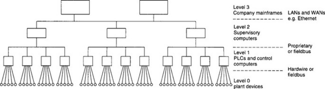
Level 0 is the actual plant, with devices linking to the next level by direct wiring or simple RS232/422 serial links.
Level 1 is the level the majority of this chapter is concerned with, consisting of PLCs and small computers directly controlling the plant.
Usually the layout is not as clear cut as this implies. There are also differences between different companies, some number the layers from top to bottom and some ignore level 0.
There are many advantages to distributed systems. The resulting tree is conceptually simple, and as such is easy to design, commission, maintain and modify. A correctly designed system will be, for short periods, fault tolerant and can cope in a limited mode with the failure of individual stations. A distributed system can also bring about an increase in performance as lower level machines take the work off higher level machines.
16.5.6 Proprietary systems
In this section we will look at a typical proprietary system used to link PLCs from the same manufacturer. Typical examples are the GEM-80s Coronet and ESP, Siemen’s Sinec and Modicon’s Modbus. For reasons of space we shall consider how machine to machine links are achieved with Allen Bradley PLC-5s which communicate with each other on a peer to peer (no master) token passing highway based on twinaxial cable and operating at 57.6Kbaud. Their trade name is Data Highway Plus. The PLC stations’ addresses are set on switches in each PLC, and up to 64 stations can exist on one line with octal addresses 0–77.
Communication is established with a single message (MSG) instruction. This can be set up to read or write a block of data, the programmer specifying:
(1) The start address at the local end;
(2) The start address at the target end;
(3) The length of the block to be transferred (in words); and
The MSG instruction appears in a program as Figure 16.77(a), the transfer being initiated every time the rung goes true. The ENable bit goes true when the transfer is started, and the DoNe bit goes true when it has been successfully completed. The ERR or flag goes true when an error occurs. Common errors are a line fault, a non existent address at the far end or the PLC at the far end shutdown. The cause of the fault is given in flags set in the message control word. Link statistics (e.g. number of retries) are kept in the processor for diagnostic purposes.
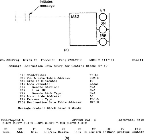
Figure 16.77 The PLC-5 Message (MSG) Instruction: (a) as written in the ladder diagram; (b) as seen in detail on the programming terminal
The details of the MSG instruction are set up by the programmer via the screen of Figure 16.77(b). These are mostly self explanatory, with the possible exception of the remote link which is concerned with sending data via a gateway module to a different highway, possibly of a different type.
The data highway is also used by the programming terminal, so a programmer can connect anywhere onto the data highway and link into any machine on the network.
16.5.7 Ethernet
Ethernet is a very popular bus based LAN originated by DEC, Xerox and Intel and is commonly used to link the computers at level 2 in Figure 16.76. It uses 50 Ω coaxial cable, with a maximum cable length of 500 m (although this can be extended with repeaters). Up to 1024 stations can be accommodated, although in practical systems the number is far lower. Baseband (i.e. non modulated) signalling is used with CSMA/CD access control. The raw data rate is 10 Mbaud, giving very fast response at loading levels up to about 20–30% of the theoretical maximum. Beyond this, collisions start to occur.
Because Ethernet uses CSMA/CD the successful transmission of a message cannot be guaranteed. It is possible, (but unlikely) for a given message to continually suffer from crashes and never get access to the network. In the jargon ethernet is ‘non determinstic’. In practice, if the network loading is kept below 30% of its theoretical capacity this is not a problem. Many PLCs (such as the PLC-5/40E) now can provide direct connection to an Ethernet network.
16.5.8 Towards standardisation
We have already discussed the difficulties of linking different equipment. There is normally little problem linking PLC networks to higher level computers. PLC manufacturers publish their message format and protocols, and interfacing software (called ‘drivers’) has been written for all common computers and PLCs. The difficulty comes when you want to link two machines from different manufacturers at level 1 in Figure 16.76. In many cases, the only economical solution is to do it through the computers and the higher level link.
General Motors (GM) in the USA were faced with this problem and attempted to specify a LAN for industrial control. This was called MAP (Manufacturing Automation Protocol). A similar office based LAN called TOP (Technical Office Protocol) was conceived at the same time. With GM’s purchasing muscle, it involved several automation equipment manufacturers. A firm commitment to the OSI model was made, and the network based on broadband token bus as specified in IEEE 802.4 was chosen as it is deterministic.
MAP, however, has not been widely adopted. There appears to be several reasons for this distinct lack of enthusiasm. The first is a bureaucratic organisation and a changing specification. The second reason is cost; MAP links often cost more than the PLC to which they are connected. The third reason is speed; by using token passing MAP is slow by comparison with other standards. The final, and perhaps most crucial, fact is that MAP seems to have settled at a level where it is in direct competition with established LANs such as Ethernet rather than the proprietary systems at level 1 of Figure 16.76.
A standardised fieldbus system would allow PLCs, sensors and actuators to be connected and communicate with minimal cost. Unfortunately at the time of writing (early 2002) a standard seems as far away as ever with progress being slowed by commercial and national infighting.
Profibus is one the more common fieldbus contenders, largely because it has been adopted by Siemens and many other German electrical companies. There are three versions of Profibus designed for three different application areas. All use token passing.
The first, called Profibus-DP, for decentralised periphery, is by far the commonest and is designed to link intelligent masters (e.g. a PLC), to slave devices such as sensors, drives or actuators. Profibus only uses levels 1 and 2 of the ISO/OSI model. Twisted pair RS485 or fibre optics are used for transmission.
The second, Profibus-FMS, for field message specification, is designed for the higher level with multiple masters and allowing peer to peer communication. Levels 1, 2 and 7 of the ISO/OSI model are used and RS485 or fibre optics for transmission.
Both DP and FMS share the same transmission standards and can consequently work together on the same network.
The final form, designed for process automation in hazardous areas, is Profibus-PA which permits the construction of an intrinsically safe network. Profibus-PA uses slightly different standards to DP and FMS, but can be linked by a segment coupler device.
All are a linear bus system, i.e. a straight line. Transmission speeds from 9.6 kbit/s (up to 1200 m) to 12 Mbit/s (up to 100 m) can be used. Screened twisted pair is used, with terminating resistors at each end of the bus. Up to 32 stations can be used in each segment, each with a unique station address. Segments can be coupled with segment repeaters, allowing a total of 127 stations to be addressed. Addresses are assigned for global or group data reducing the number of messages and time lag problems when data for several devices are to be changed together.
Connections to masters or slaves are made via standard 9 pin D-type connectors, as shown on Figure 16.78(a). Terminating resistors are either switched in internally at the end stations or connected inside the final plugs. Note that the terminating resistors require power, this normally comes from the end stations themselves.
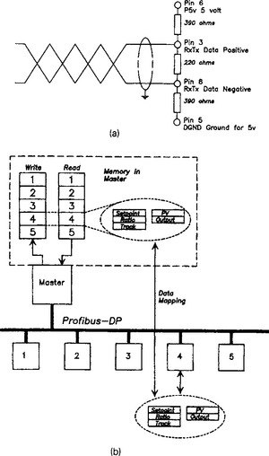
Figure 16.78 Profibus-DP network: (a) connection at a Profibus device. Non terminating devices use only pins 3 and 8; (b) mapping between a Profibus device and memory in the network master
The manufacturer of each device on the network, e.g. a VF drive, provides a disc file, called the GSD, which is a description of the data exchange the device can support (e.g. accepting speed reference and run command and providing load current and drive state etc.) plus operating parameters such as supported transmission speeds. Included in the GSD file is a unique identification number assigned by the Profibus User Organisation. The GSD files for all the devices on the network are used along with the station addresses to build a network description which is held in the master.
Because Profibus-DP only uses levels 1 and 2, the data exchange maps onto pre-determined areas in the master controller (usually a PLC) as shown on Figure 16.78(b). To change the speed of the drive, the user simply writes the new speed into the mapped area, and the data is transferred with no further action. In a similar manner, slave data and status is automatically read from the mapped area. A Profibus-DP network is thus totally transparent to the user.
A typical example of the problems that any attempts to specify a standardised fieldbus system may encounter is the continual introduction of new ideas. All the communications systems described so far are based on what is called the source/destination model. If station A has information for station B, a message is sent with the format:
![]()
If this information is to be sent to several stations, each will need their own message. In applications where multiple setpoints have to be sent to multiple controllers, the delay caused by the time shift between the messages can cause problems, although this can be overcome to some extent by the use of group or global addresses as used by Profibus.
In addition, if station A needs information from station B, (the state of an interlock for example), station A must perform a read on each occasion the data is required.
A recent development, called the producer/consumer model, uses a different approach. Here data is placed onto the network with no indication as to who it is for. The format is now simply:
![]()
All stations using this data accept it at the same time, eliminating the need for multiple messages. This significantly reduces the number of messages and hence increases the network speed.
The placement of data onto the network can be done in two ways. The first, and fastest, is ‘notify on change’. Here a station only places information on the network when a new value is different than the old. Stations with an interest in this data assume that the status or value remains the same until notified otherwise. There are obvious dangers in this, and a regular pre-defined ‘heartbeat’ is included to say a station is active on the network. The second approach updates on a time basis, each data item having its own, or a global, update time.
At the time of writing, Foundation Fieldbus is the only producer/consumer fieldbus network, and Rockwell (Allen Bradley) have also adopted the method for their proprietary ControlNet. The latter is interesting as it combines the ideas of their remote I/O and Data Highway onto one system and allows PLC racks, (and their data), to be shared equally amongst several processors and not dedicated to one as before.
16.6 Graphics
Operator controls are being increasingly provided by computer graphic screens. These can be a display device designed specifically for a particular range of PLCs (for example the Allen Bradley Panelview and the CEGELEC Imagem) and general purpose graphic display devices (such as ABB/ASEA’s excellent Tesselator) or graphics software running on conventional personal computers. Figure 16.79 shows some typical examples.
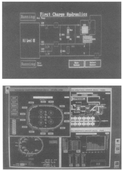
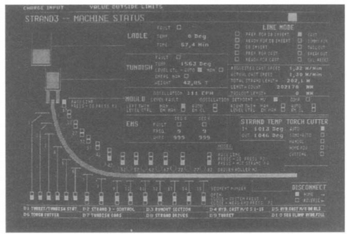
Figure 16.79 Various graphic displays: (a) Allen Bradley touchscreen Panelview using block graphics; (b) high resolution Scada system; (c) the ABB Tesselator. Photos courtesy of Co-Steel Sheerness, Scomagg and ABB
The major advantages are simplicity of installation and flexibility. A graphics terminal has just two connections to the outside world, a serial link connection and a power supply. If it is used to replace a desk full of switches and indicators there are obvious cost savings.
The designer of desks or control stations often has to deal with changes and modifications. Constructing a desk is always a fine balance of time, choosing between waiting until all the requirements are clear, and the minimum time needed to make it. Modifications at the commissioning stage rarely look neat. The displays on a graphical terminal can be modified relatively easily, and, more importantly, the modifications leave no scars. If the design of a normal desk can only start when the desk contents are 95% finalised (which is about right) a graphic screen can be started at 75% finalised. This flexibility is of great assistance as no job is ever right first time.
There are disadvantages, though. The most important of these is the limited amount of information that can be displayed on a single screen. It is very easy to overcrowd a screen (giving a screen similar to a page full of text on a word processor) making it difficult for the operator to identify critical items. A useful rule of thumb is not to use more than 25–30% of the screen.
The effect of this is often a need to build up a hierachy of screens; the top screen showing an overview, lower screens showing more and more detail. The problem with this is the time delay needed to shift through the screens. Direct screen to screen movement is possible by calling for a page number (which needs a good human operator memory, or a directory piece of paper, or wasted screen space) or by making all screen changes via an intermediate directory page (with additional delay). These time delays are small (less than a second typically) but the cumulative annoyance is large.
The time taken to update screen data can also be problematical, particularly where a machine to machine link is involved. Again a response time of around one second is typical, but several seconds is by no means uncommon. The use of a graphic terminal for fault finding on a fast moving plant is not really feasible.
There are generally two types of graphic terminal. The simplest, known as block graphics, has one store location for each character position on the screen and approximates to the old CGA standard on a personal computer.
The second type of display deals not with individual characters, but with individual points on the screen called ‘pixels’. A typical medium resolution screen will have 640 (horizontal) by 480 (vertical) pixels, a total of 307 200 points. Each of these can be accessed individually, allowing lines to be drawn at any angle, fill patterns of any type to be used and trend graphs of plant variables to be displayed. Each individual pixel can have its own colour (from over 256 possible colours in some displays) and intensity. The result is an almost photographic resolution. There are additional costs, the most obvious of which is a large store requirement. The system hardware and software is more complex (and hence more expensive) but, perhaps surprisingly, this is not apparent to the designer. Programming for these screens is surprisingly simple with instructions using keywords like
![]()
or pick and place functions similar to a good commercial graphics package.
Supervisory Control and Data Acquisition (SCADA) systems are based around graphical objects which are linked to variables in the control systems. The state of the objects on the screen (e.g. size, colour, rotation, etc.) can be changed according to the the values of the variables in the control systems giving a very visual image of the operation.
The environment around a display needs to be carefully considered. Most screens are mounted angled up, and are prone to annoying reflections from overhead lights and windows. Bright lighting (and above all direct sunlight) can make a display impossible to read. Displays are also adversely affected by magnetic fields. Close proximity to electric motors, transformers or high current cables will cause a picture to wobble and the colours to change. The effect can be overcome by screening the monitor with a mu-metal cage). Flat screen TFT or LCD displays do not suffer from this effect.
The size and weight of the monitors are often overlooked making them difficult to mount neatly, and even more difficult to change. Access should be made as easy as possible; trying to hold a 25 kg display in place with one hand whilst undoing interminably long mounting screws is not much fun.
Displays fail, and the implication of this needs to be considered in the design. If all the plant control is performed by screens, what will happen during the ten or so minutes it will take to locate a spare and change the faulty unit? Often dual displays are used to overcome this problem.
The operator will obviously need to input data and initiate actions. Keyboards are one approach, but many people are nervous of them and the cable connecting the keyboard always seems prone to damage. In dirty environments keys can become blocked with dirt and membrane keypads with tactile (feel) feedback should be used.
If the operator has to access points anywhere on the screen, a tracker ball is a useful device. Rather like an upside down mouse it controls the movement of a cursor on the screen. All normal actions can be performed with three buttons on the trackerball and a numerical keypad. Trackerballs work surprisingly well in dirty environments as they are open underneath and dirt seems to fall straight through. Mice perform a similar function but are vulnerable to damage and dirt and seem more suited to an office environment.
A final consideration is security. Most modern graphics systems are based on good quality personal computers. These have value outside of industry and are vulnerable to theft. Often is it is not the PCs or screens which are stolen, but the internal motherboards and memory cards. Suitable security methods should be used if a PC based system is to be left unattended for a period of time (e.g. during a Christmas shutdown). Needless to say backups should not be stored on the same PC as the original system.
16.7 Software engineering
Any project goes through six stages during its life. The first of these, analysis, is studying the application to understand what is required. This is by far the most difficult stage as the project requirements are usually unclear. Most projects that come unstuck do so because this first stage has been cut short or overlooked.
Next comes specification, which is documenting the analysis so everyone concerned can agree what is to be done and what the end result should be. If you can’t produce a specification, how can you sensibly design it? Never say ‘we’ll sort that out later’ because later becomes 3 a.m. as the plant starts up. The final testing procedures must also be defined at the specification stage; again if you don’t know how you will test it, how will you know if it’s working properly? Defining testing procedures in the cold light of day several months before the final frantic rush to meet a deadline also helps the poor commissioning engineer to resist the pleas for a premature start up.
The importance of these two first stages cannot be over-emphasised, too often the users do not know, or do not say, what they want, but once the project is complete they are sure it wasn’t that. With these first two difficult stages over, the rest of the project becomes much easier!
The design stage can now start, (simple with a good specification) followed by installation. Next comes commissioning. These can also be difficult times, as in any project the control engineer ends up collecting everybody’s delays and comes under pressure to ‘get the plant away’. It is here that the advantage of the test schedule from the specification stage will be invaluable.
It is not generally understood that commissioning involves both positive and negative testing. Positive testing is obvious; it is ensuring that when the firkling button is pressed the plant firkles. Practically everyone sees the need for this. Negative testing is less obvious; it is ensuring that the control system deals correctly with all the unlikely circumstances and fault conditions. Negative testing takes far far longer, because there are many more fault modes than healthy modes. It is very common for people to say ‘it works, let’s go’ when only the positive testing has been done. Try to resist this pressure, at best it can lead to damaged plant a few years hence, at worse some safety features could be overlooked.
Finally the plant is handed over to the maintenance department. In commercial software it is generally thought that over 50% of the effort goes into maintenance as changes are made to meet new requirements or correct the inevitable bugs. For easy maintenance all the documentation must be complete and up to date.
16.8 Safety
Most industrial processes are hazardous, and the safety of all personnel must be of prime importance. This section is a personal view and can only give a simple discussion of safety considerations. The topic of safety is covered by both criminal and civil law. The designer and user of any system must therefore consult the relevant legislation and codes of practice to ensure compliance.
Every single person has a safety responsibility. Employers have a ‘duty of care’ for their employees and the public and must ensure the plant is kept in a safe condition, safe working procedures are devised for all conceivable activities, and training in these procedures provided for all relevant employees. Suppliers must ensure their equipment meets safety criteria, and draw the attention of purchasers to unavoidable hazards (protection and labelling of parts which are live during normal operation for example). Employees must follow safety procedures and not expose themselves (or others) to danger. These responsibilities are covered by the Health and Safety at Work Act 1974 (HASWA) which makes the universal responsibility for safety absolutely clear.
More recently in 1992 a block of EEC Health & Safety Regulations (commonly known as the ‘six pack’) introduced the idea of risk assessment. This recognises the need to balance the cost and complexity of the safety system against both the likelihood and severity of injury. The procedures outlined use common terms with specific definitions:
| Hazard | The potential to cause harm. |
| Risk | A function of the likelihood of the hazard occurring and the severity. |
| Danger | The risk of injury. |
and outlines procedures to achieve acceptable safety standards. Risk assessment is a legal requirement under most modern legislation, and is covered in detail in standard prEN1050 ‘Principles of Risk Assessment’.
A Health & Safety Executive study of safety in control systems (‘Out of Control’ HSE books 1995 ISBN 0717608476) makes worrying reading. It suggests that more than 60% of safety related failures are introduced into a system before it is taken into service for the first time. Approximately 44% of safety incidents come from specification errors, 15% from design errors and 6% from poorly thought out changes during commissioning.
The inclusion of a programmable controller brings additional hazards (and solutions) which must be recognised. A PLC can introduce potentially dangerous situations in different ways. The first (and probably commonest) route is via logical errors in the program. These can be the result of oversight, or misunderstanding, on behalf of the original designer who did not appreciate that this set of actions could be dangerous, or by later modifications by people who deliberately (or accidentally) removed some protection to overcome a failure in the middle of the night. ‘Midnight programming’ is particularly worrying as usually the only person who knows it has been done is the offending person, and the danger may not be apparent until a considerable time passes and the hazardous condition occurs.
The second possible cause is failure of the input and output modules; in particular the components connected directly to the plant which will be exposed to high voltage interference (and possibly direct connected high voltages in the not unlikely event of cable damage). Output modules can also suffer high currents in the (again not unlikely) event of a short circuit. Typical output devices are triacs, thyristors or transistors. The failure mode of these cannot be predicted; all can fail short circuit or open circuit. In these failure conditions the PLC would be unable to control the outputs. Similarly an input signal card can fail in either the ‘on’ or ‘off’ state, leaving the PLC misinterpreting a possibly important signal.
The next failure mode is the PLC itself. This can be further divided into hardware, software and environmental failures. A hardware failure is concerned with the machine itself; its power supply, its processor, the memory (which contains the ‘personality’ of the PLC, the user’s program, and the data storage). Some of these failures will have predictable effects; a power supply failure will cause all outputs to de-energise, and the PLC supplier will have included memory checks in the design. Environmental effects arise from peculiarities in the installation such as dust, humidity, temperature (and rapid temperature changes) possible water ingress and vibration, and these can result in unexpected operation of output devices.
The final cause is electrical interference (usually called noise). Internally almost all PLCs work with 5 V signals, but are surrounded by high voltage high current devices. Noise can cause input signals to be misread by the PLC, and in extreme cases can corrupt the PLC’s internal memory. PLCs generally have internal protection against memory corruption and noise on remote I/O serial lines, so the usual effect of noise is to cause a PLC to stop (and outputs to de-energise). This cannot, however, be relied upon.
Figure 16.80 shows a normal motor starter circuit built without a PLC. Safety precautions here are:
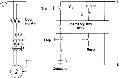
Figure 16.80 A standard hardwired motor starter for a low risk application. This would normally be considered to be sate. In higher risk applications there would probably be dual connections on the emergency stop button, dual contactors and the state of the contactors would be monitored by the emergency stop relay
• Isolation switch at the MCC removes the supply for maintenance work.
• Normally closed contacts on the stop and emergency stop buttons. A broken wire will look like a stop button being pressed, as will loss of the control supply.
• If the emergency stop is pressed and released, the motor does not restart.
It is still possible to identify dangerous failure modes in this system. The button head of the emergency stop button could unscrew and fall off, or the contacts of the contactor could weld made, or a short could occur between the cores to the stop button but these failure modes are exceedingly rare, and Figure 16.80 would be generally accepted as safe for use in normal circumstances.
In Figure 16.81(a) the same functions have been provided by an unsafe PLC system. To save costs the MCC door isolator has been replaced by a simple switch which makes to say ‘Isolate’. Similarly normally open contacts have been used for stop and emergency stop. This is controlled by the unsafe program of Figure 16.81(b).
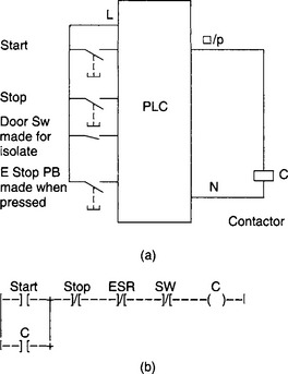
Figure 16.81 An unsafe PLC based system totally reliant on software. The dangers of this system only become apparent when failures occur
It is important to realise that to the casual user, Figures 16.80 and 16.81 behave in an identical manner. The differences (and dangers) come in fault, or unusual, conditions. In particular:
• A person using a programming terminal can force inputs or outputs and over-ride the isolation. Although it is unlikely that anyone would do this deliberately, it is easy to confuse similar addresses and swop digits by mistake (forcing 0:23/01 instead of 0:32/01 for example).
• A loss of the input control supply during running will mean the motor cannot be stopped by any means other than totally removing the supply to the system.
• The system is very vulnerable to input and output card faults.
None of these are apparent to the user until an emergency occurs.
A prime rule, therefore, for using PLCs is:
‘The system should be at least as safe as a conventional system’
Figure 16.82(a) is a revised PLC version of Figure 16.80. The isolator has been re-instated with an auxiliary contact as PLC inputs, and normally closed contacts used for the stop and emergency stop buttons. An auxiliary contact has been added to the starter, and this is used to latch the PLC program of Figure 16.82(b). The emergency stop is hardwired into the output and is independent of the PLC, and on release the motor will not restart (because the latching auxiliary contact in the program will have been lost). On loss of control supply the program will think the stop button has been pressed, and the motor will stop. Figure 16.82 thus behaves in failure as Figure 16.80.
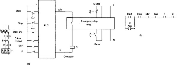
Figure 16.82 A safe PLC system for low risk applications. As for Figure 16.80 more features could be added if the risk was higher
Although this example is simple, it illustrates the necessary analysis and considerations that must be applied in more complex systems.
Complex electronic systems can bring increased safety. Consider a thyristor drive controlling the speed of a large d.c. motor. In a typical arrangement there will be an upstream a.c. contactor to enable the drive. Hardwire connection of an emergency stop button into the a.c. contactor will obviously stop the drive, but the inertia of the motor and the load will keep it rotating for several seconds. A thyristor drive, however, can stop the load in less than one second by regeneratively braking the motor, but this requires the drive to be alive and functional. The operation of the emergency stop implies a dangerous condition in which the fastest possible stop is required. It is almost certain that at this time the drive controls are functional and there are no ‘latent’ faults.
Here the emergency stop can operate in two ways. First it initiates an electronic regenerative crash stop via the control system which should stop the drive in less than one second. The emergency stop also releases a delay drop out hardwire relay set for 1.5 s which releases the a.c. contactor. This gives the safest possible reaction to the pressing of the emergency stop button. Safety considerations do not therefore, explicitly require relay based, non electronic hardware, but the designer must be prepared to justify the design decisions and the methods used.
Where complex control systems are to be used, a common method of improving safety is to duplicate sensors, control systems and actuators. This is known as redundancy. A typical application occurs in boilers where feed water is held in a drum. Deviations in water level are dangerous; too low and the boiler will overheat, possibly to the point of melting the boiler tubes; too high and water can be carried over to the downstream turbine with risk of catastrophic blade failure. High and low level sensors are therefore usually provided with each being duplicated. The safety system reacts to any fault signal, so two sensors have to fail for a dangerous condition to arise. If the probability of a sensor failure in time T is p (where 0 < p < 1) the probability of both failing is p2. In a typical case, p will be of the order of 10−4 failure per year giving p2 of 10−8.
There are two disadvantages. The first is that a sensor can fail into a permanently safe signal state, and this failure will be ‘latent’, i.e. hidden from the user with the plant running on one sensor. The second problem is that the plant reliability will go down, since the number of sensors goes up and any sensor failure can result in a shutdown. Both of these effects can be reduced by using ‘majority voting’ circuits, taking the vote of two out of three or three out of five signals.
Redundancy can be defeated by ‘common mode’ failures. These are failures which affect all the parallel paths simultaneously. Power supplies, electrical interference on cables following the same route and identical components from the same batch from the same supplier are all prone to common mode failure. For true protection, diverse redundancy must be used, with differences in components, routes and implementation to reduce the possibility of simultaneous failure.
To give true redundancy it is sensible to provide duplication in the control system as well to protect against hardware and software failures in the system itself. Duplicate control schemes, though, are vulnerable to a form of common mode failure called a ‘systematic failure’. Suppose duplicated temperature sensors are compared, inside a PLC program, with an alarm temperature. Suppose both are identical devices, running the same program containing a bug which inadvertently (but rarely so it does not show up during simple testing) changes the setting for the alarm temperature (from 60°C say, to 32053°C). Such an effect could easily occur by a mistype in a MOVE instruction in a totally unrelated part of the program. This error will affect both control systems, and totally remove the redundancy.
If reliance is being made on redundant control systems, therefore, they should be totally different; different machines with different I/O and different programs written by different people with the machines installed running on different power supplies with different types of sensors connected by different cable routes.
The Health and Safety Executive (HSE) became concerned about the safety of direct plant control with computers, and produced an occasional paper OP2 ‘Microprocessors in Industry’ in 1981. This was followed in 1987 by two booklets ‘Programmable Electronics Systems in Safety Related Applications’. Book 1 (an Introductory Guide) is a general discussion of the topic, and Book 2 (General Technical Guidelines) goes through the necessary design stages. They suggest a five stage process:
(i) Perform a hazard analysis of the plant or process;
(ii) From this, identify which parts of the control system are concerned with safety and which are concerned purely with efficient production. The latter can be ignored for the rest of the analysis;
(iii) Determine the required safety level (based on accepted attainable standards or published material);
(iv) Design safety systems to meet or exceed these standards; and
(v) Assess the achieved level (by using predicted probability of failure for individual parts of the design). Revise the design if the required level has not been achieved.
The books stress the importance of ‘Quality’ in the design; quality of components, quality of the suppliers and so on.
The IEC standard IEC 61508 Functional Safety of Electrical/Electronic/Programmable electronic safety related systems covers similar grounds to the HSE books. This is based on the ideas of safety functionality (what it is designed to protect against and how the protection is achieved e.g. ‘open quench valve if temperature rises above 250°C’) and the Safety Integrity Level (or SIL) which, somewhat simplified, is the probability, p, that the safety system will fail to operate on demand. The SIL covers the entire safety system including sensors, control system, and actuators. Four SILs are defined from a basic SIL-1 (10−1 > p > 10−2) to SIL-4 (10−4 > p > 10−5). The required SIL is determined from a risk assessment of the system. For continuous protection on a hazardous plant the normal requirement is SIL-3 or SIL-4. Guidelines for architectural constraints (such as keeping the safety system separate from the control system, and using redundancy) are also given. It is probable that IEC 61508 will become a European standard in the near future, and the two HSE books are being re-written to incorporate ideas from IEC 61508.
Surprisingly some fieldbus systems (e.g. specialist versions of Profibus and Safety Bus from Pilz) can achieve SIL-3 which makes a fieldbus safety system attractive in hazardous applications. Extreme care must, of course, be taken.
In America, the Instrument Society of America (ISA) standard S84 follows broadly similar lines to the HSE guidelines and IEC 61508.
Because the HSE books, IEC 61508 and S84 are standards they have the legal status of guidance notes and there is no formal requirement to follow them. In the event of an incident, however, the designers and users must be prepared to justify the actions they have taken and conformance with good practice is a legal defence.
Very high safety levels can be achieved with some PLCs. Siemens market the 115F PLC which has been approved by the German TUV Bayern (Technical Inspectorate of Bavaria) for use in safety critical applications such as transport systems, underground railways, road traffic control and public elevators. The system is based on two 115 PLCs and is a model of diverse redundancy. The two machines run diverse system software and check each other’s actions. There is still a responsibility on the user to ensure that no systematic faults exist in the application software.
Inputs are handled as Figure 16.83. Diverse (separate) sensors are fed from a pulsed output. A signal is dealt with only if the two processors agree. Obviously the choice of sense of the signal for safety is important. For an overtravel limit, for example, the sensors should be made for healthy and open for a fault.

Actuators use two outputs (of opposite sense) and two inputs to check the operation as Figure 16.84. Each sub-unit checks the operation of the other by brief pulsing of the outputs allowing the circuit to detect cable damage, faulty output modules and open circuit actuators. If, for example, output B fails on, both inputs A and B will go high in the Off state (but the actuator will safely de-energise.)
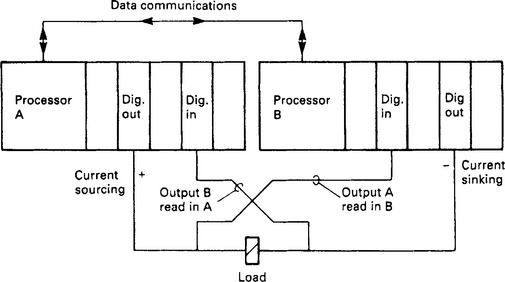
The operation of Figures 16.83 and 16.84 is straightforward, but it should not be taken as an immediately acceptable way of providing a fail-safe PLC. The 115F is truly diverse redundant, even the internal integrated circuits are selected from different batches and different manufacturer, and it contains well tested diverse self checking internal software. A DIY system would not have these features, and could be prone to common mode or systematic failures.
A PLC system is an electrical system, and is subject to the same legislation as conventional electrical schemes. Apart from the Health and Safety at Work Act, the designer should also observe the Institute of Electrical Engineers Wiring Regulations, and the Electricity at Work Regulations 1990.