Units, Mathematics and Physical Quantities
MA Laughton, BASc, PhD, DSc(Eng), FREng, CEng, FIEE, Formerly of Queen Mary & Westfield College, University of London (Section 1.2.10)
This reference section provides (a) a statement of the International System (SI) of Units, with conversion factors; (b) basic mathematical functions, series and tables; and (c) some physical properties of materials.
1.1 International unit system
The International System of Units (SI) is a metric system giving a fully coherent set of units for science, technology and engineering, involving no conversion factors. The starting point is the selection and definition of a minimum set of independent ‘base’ units. From these, ‘derived’ units are obtained by forming products or quotients in various combinations, again without numerical factors. For convenience, certain combinations are given shortened names. A single SI unit of energy (joule = kilogram metre-squared per second-squared) is, for example, applied to energy of any kind, whether it be kinetic, potential, electrical, thermal, chemical …, thus unifying usage throughout science and technology.
The SI system has seven base units, and two supplementary units of angle. Combinations of these are derived for all other units. Each physical quantity has a quantity symbol (e.g. m for mass, P for power) that represents it in physical equations, and a unit symbol (e.g. kg for kilogram, W for watt) to indicate its SI unit of measure.
1.1.1 Base units
Definitions of the seven base units have been laid down in the following terms. The quantity symbol is given in italic, the unit symbol (with its standard abbreviation) in roman type. As measurements become more precise, changes are occasionally made in the definitions.
Length: l, metre (m) The metre was defined in 1983 as the length of the path travelled by light in a vacuum during a time interval of 1/299 792458 of a second.
Mass: m, kilogram (kg) The mass of the international prototype (a block of platinum preserved at the International Bureau of Weights and Measures, Sevres).
Time: t, second (s) The duration of 9 192 631 770 periods of the radiation corresponding to the transition between the two hyperfine levels of the ground state of the caesium-133 atom.
Electric current: i, ampere (A) The current which, maintained in two straight parallel conductors of infinite length, of negligible circular cross-section and 1 m apart in vacuum, produces a force equal to 2 × 10⁻⁷ newton per metre of length.
Thermodynamic temperature: T, kelvin (K) The fraction 1/273.16 of the thermodynamic (absolute) temperature of the triple point of water.
Luminous intensity: I, candela (cd) The luminous intensity in the perpendicular direction of a surface of 1/600000 m2 of a black body at the temperature of freezing platinum under a pressure of 101 325 newton per square metre.
Amount of substance: Q, mole (mol) The amount of substance of a system which contains as many elementary entities as there are atoms in 0.012kg of carbon-12. The elementary entity must be specified and may be an atom, a molecule, an ion, an electron …, or a specified group of such entities.
1.1.2 Supplementary units
Plane angle: α, β …, radian (rad) The plane angle between two radii of a circle which cut off on the circumference of the circle an arc of length equal to the radius.
Solid angle: Ω, steradian (sr) The solid angle which, having its vertex at the centre of a sphere, cuts off an area of the surface of the sphere equal to a square having sides equal to the radius.
1.1.3 Notes
Temperature At zero K, bodies possess no thermal energy. Specified points (273.16 and 373.16 K) define the Celsius (centigrade) scale (0 and 100°C). In terms of intervals, 1°C = 1K. In terms of levels, a scale Celsius temperature θ corresponds to (θ+273.16) K.
Force The SI unit is the newton (N). A force of 1 N endows a mass of 1 kg with an acceleration of 1 m/s2.
Weight The weight of a mass depends on gravitational effect. The standard weight of a mass of 1 kg at the surface of the earth is 9.807 N.
1.1.4 Derived units
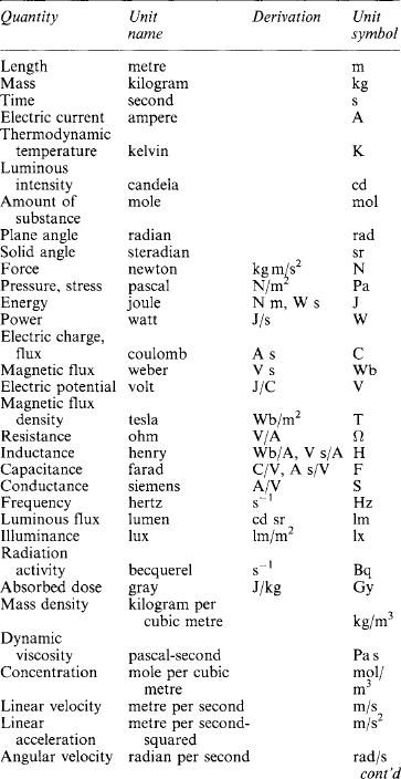
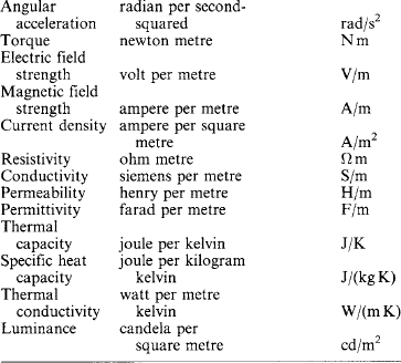
All physical quantities have units derived from the base and supplementary SI units, and some of them have been given names for convenience in use. A tabulation of those of interest in electrical technology is appended to the list in Table 1.1.
Decimal multiples and submultiples of SI units are indicated by prefix letters as listed in Table 1.2. Thus, kA is the unit symbol for kiloampere, and μF that for microfarad. There is a preference in technology for steps of 103. Prefixes for the kilogram are expressed in terms of the gram: thus, 1000 kg = 1 Mg, not 1 kkg.

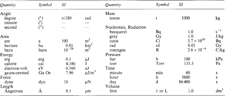
1.1.5 Auxiliary units
Some quantities are still used in special fields (such as vacuum physics, irradiation, etc.) having non-SI units. Some of these are given in Table 1.3 with their SI equivalents.
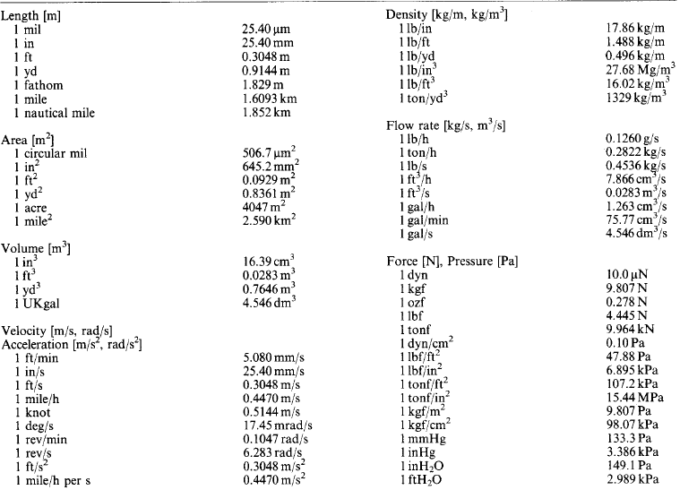
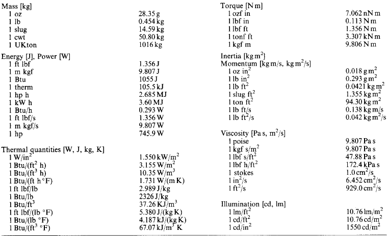
1.1.6 Conversion factors
Imperial and other non-SI units still in use are listed in Table 1.4, expressed in the most convenient multiples or submultiples of the basic SI unit [ ] under classified headings.
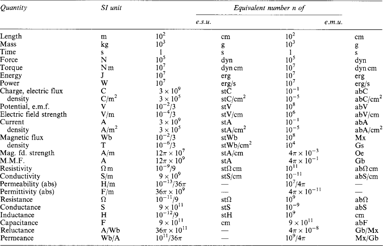
1.1.7 CGS electrostatic and electromagnetic units
Although obsolescent, electrostatic and electromagnetic units (e.s.u., e.m.u.) appear in older works of reference. Neither system is ‘rationalised’, nor are the two mutually compatible. In e.s.u. the electric space constant is μ0 = 1, in e.m.u. the magnetic space constant is μ0 = 1; but the SI units take account of the fact that ![]() is the velocity of electromagnetic wave propagation in free space. Table 1.5 lists SI units with the equivalent number n of e.s.u. and e.m.u. Where these lack names, they are expressed as SI unit names with the prefix ‘st’ (‘electrostatic’) for e.s.u. and ‘ab’ (‘absolute’) for e.m.u. Thus, 1 V corresponds to 10−2/3 stV and to 108 abV, so that 1 stV = 300 V and 1 abV = 10−8 V.
is the velocity of electromagnetic wave propagation in free space. Table 1.5 lists SI units with the equivalent number n of e.s.u. and e.m.u. Where these lack names, they are expressed as SI unit names with the prefix ‘st’ (‘electrostatic’) for e.s.u. and ‘ab’ (‘absolute’) for e.m.u. Thus, 1 V corresponds to 10−2/3 stV and to 108 abV, so that 1 stV = 300 V and 1 abV = 10−8 V.
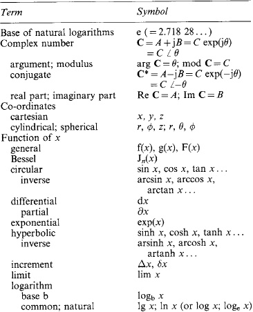
1.2 Mathematics
Mathematical symbolism is set out in Table 1.6. This subsection gives trigonometric and hyperbolic relations, series (including Fourier series for a number of common wave forms), binary enumeration and a list of common derivatives and integrals.
1.2.1 Trigonometric relations
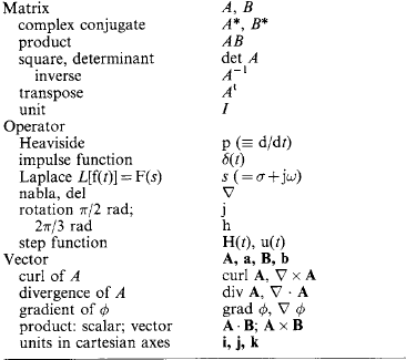
The trigonometric functions (sine, cosine, tangent, cosecant, secant, cotangent) of an angle θ are based on the circle, given by x2+y2 = h2. Let two radii of the circle enclose an angle θ and form the sector area Sc = (πh2)(θ/2π) shown shaded in Figure 1.1 (left): then θ can be defined as 2Sc/h2. The right-angled triangle with sides h (hypotenuse), a (adjacent side) and p (opposite side) give ratios defining the trigonometric functions
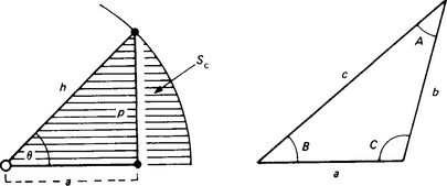
In any triangle (Figure 1.1, right) with angles, A, B and C at the corners opposite, respectively, to sides a, b and c, then A+B+C = π rad (180°) and the following relations hold:
Other useful relationships are:
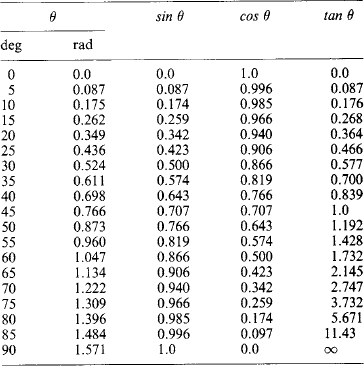
Values of sin θ, cos θ and tan θ for 0° < θ < 90° (or 0 < θ < 1.571 rad) are given in Table 1.7 as a check list, as they can generally be obtained directly from calculators.
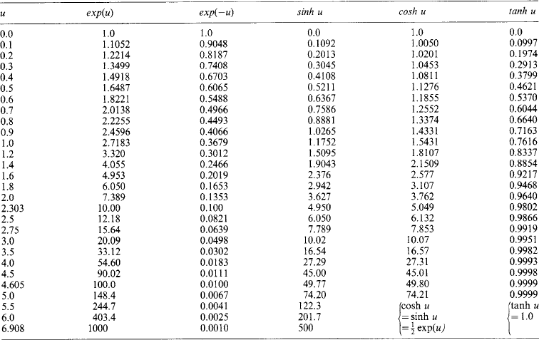
1.2.2 Exponential and hyperbolic relations
Exponential functions For a positive datum (‘real’) number u, the exponential functions exp(u) and exp(−u) are given by the summation to infinity of the series
with exp(+ u) increasing and exp(−u) decreasing at a rate proportional to u.

In the electrical technology of transients, u is most commonly a negative function of time t given by u = −(t/T). It then has the graphical form shown in Figure 1.2 (left) as a time dependent variable. With an initial value k, i.e. y = k exp(−t/T), the rate of reduction with time is dy/dt = −(k/T)exp(−t/T). The initial rate at t = 0 is −k/T. If this rate were maintained, y would reach zero at t = T, defining the time constant T. Actually, after time T the value of y is k exp(−t/T) = k exp(−1) = 0.368k. Each successive interval T decreases y by the factor 0.368. At a time t = 4.6T the value of y is 0.01k, and at t = 6.9T it is 0.001k.
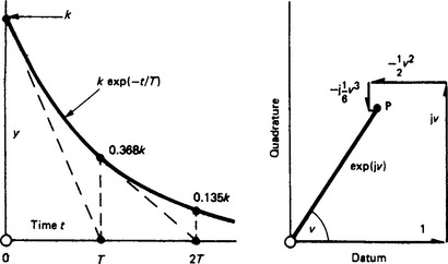
If u is a quadrature (‘imaginary’) number ±jv, then
because j2 = −1, j3 = − j1, j4 =+1, etc. Figure 1.2 (right) shows the summation of the first five terms for exp(j1), i.e.
a complex or expression converging to a point P. The length OP is unity and the angle of OP to the datum axis is, in fact, 1 rad. In general, exp(jv) is equivalent to a shift by ∠v rad. It follows that exp(±jv) = cos v ± j sin v, and that
For a complex number (u+jv), then
Hyperbolic functions A point P on a rectangular hyperbola (x/a)2 − (y/a)2 = 1 defines the hyperbolic ‘sector’ area Sh = ½a2 ln[(x/a − (y/a)] shown shaded in Figure 1.3 (left). By analogy with θ = 2Sc/h2 for the trigonometrical angle θ, the hyperbolic entity (not an angle in the ordinary sense) is u = 2Sh/a2, where a is the major semi-axis. Then the hyperbolic functions of u for point P are:
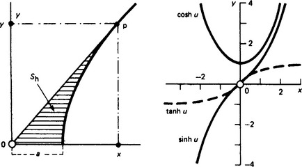
The principal relations yield the curves shown in the diagram (right) for values of u between 0 and 3. For higher values sinh u approaches ±cosh u, and tanh u becomes asymptotic to ±1. Inspection shows that cosh(−u) = cosh u, sinh(-u) = −sinh u and cosh2 u- sinh2 u = 1.
The hyperbolic functions can also be expressed in the exponential form through the series
Exponential and hyperbolic functions of u between zero and 6.908 are listed in Table 1.8. Many calculators can give such values directly.
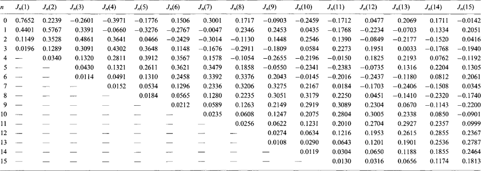
1.2.3 Bessel functions
Problems in a wide range of technology (e.g. in eddy currents, frequency modulation, etc.) can be set in the form of the Bessel equation
and its solutions are called Bessel functions of order n. For n = 0 the solution is
Table 1.9 gives values of Jn(x) for various values of n and x.
1.2.4 Series
Factorials In several of the following the factorial (n!) of integral numbers appears. For n between 2 and 10 these are
| 2!= 2 | 1/2! = 0.5 |
| 3!= 6 | 1/3! = 0.1667 |
| 4!= 24 | 1/4! = 0.417 × 10⁻¹ |
| 5!= 120 | 1/5! = 0.833 × 10⁻² |
| 6!= 720 | 1/6! = 0.139 × 10⁻² |
| 7!= 5040 | 1/7!=0.198 × 10−3 |
| 8!= 40320 | 1/8! = 0.248 × 10⁻⁴ |
| 9!= 362880 | 1/9! = 0.276 × 10⁻⁵ |
| 10! = 3628800 | 1/10! = 0.276 × 10⁻⁶ |
Arithmetic a+(a+d)+(a+2d)+ … +[a+(n − 1)d] = ½ n (sum of 1st and n th terms)
Geometric a+ar+ar2+…+arn−1 = a(1 − rn)/(1−r)
Trigonometric See Section 1.2.1.
Exponential and hyperbolic See Section 1.2.2.
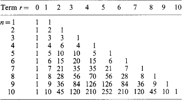
Binomial coefficients n!/[r! (n-r)!] are tabulated:
Power If there is a power series for a function f(h), it is given by

Bessel See Section 1.2.3.
Fourier See Section 1.2.5.
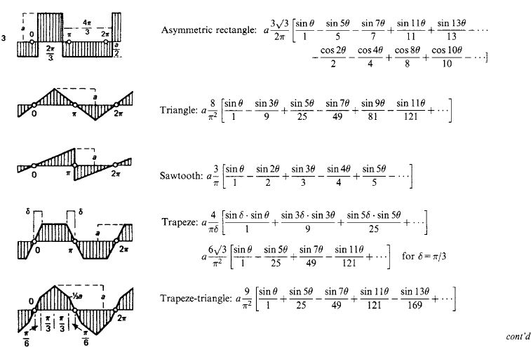
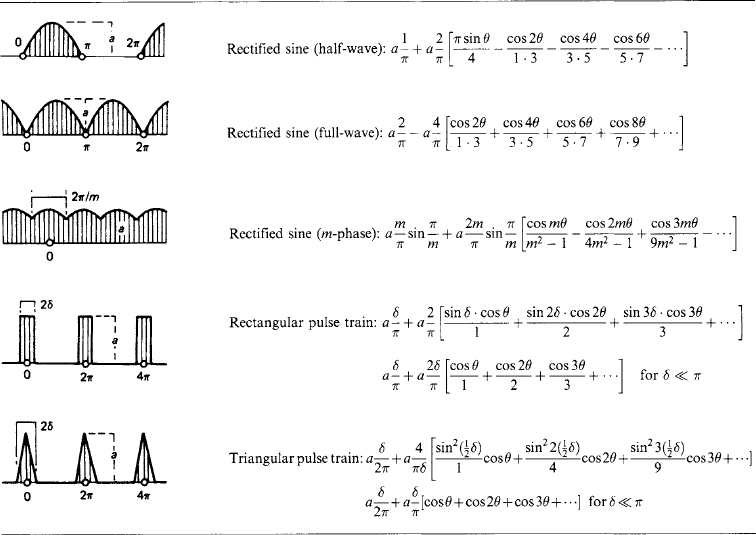
1.2.5 Fourier series
A univalued periodic wave form f(θ) of period 2π is represented by a summation in general of sine and cosine waves of fundamental period 2π and of integral harmonic orders n (= 2, 3, 4, …) as
The mean value of f(θ) over a full period 2π is
and the harmonic-component amplitudes a and b are
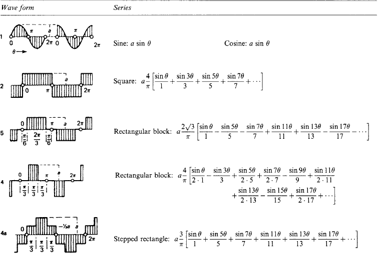
Table 1.10 gives for a number of typical wave forms the harmonic series in square brackets, preceded by the mean value c0 where it is not zero.
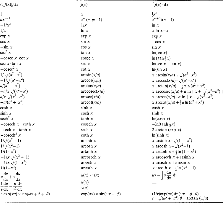
1.2.6 Derivatives and integrals
Some basic forms are listed in Table 1.11. Entries in a given column are the integrals of those in the column to its left and the derivatives of those to its right. Constants of integration are omitted.
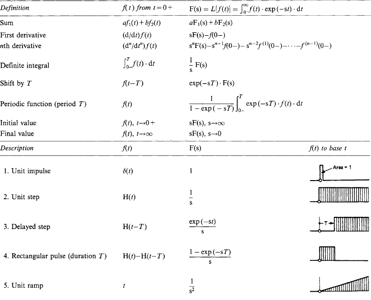
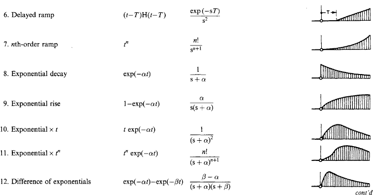
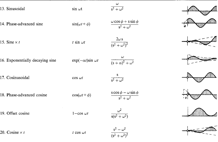
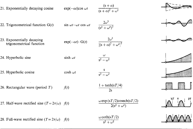
1.2.7 Laplace transforms
Laplace transformation is a method of deriving the response of a system to any stimulus. The system has a basic equation of behaviour, and the stimulus is a pulse, step, sine wave or other variable with time. Such a response involves integration: the Laplace transform method removes integration difficulties, as tables are available for the direct solution of a great variety of problems. The process is analogous to evaluation (for example) of y = 2.13.6 by transformation into a logarithmic form log y = 3.6 × log(2.1), and a subsequent inverse transformation back into arithmetic by use of a table of antilogarithms.
The Laplace transform (L.t.) of a time-varying function f(t) is
and the inverse transformation of F(s) to give f(t) is
The process, illustrated by the response of a current i(t) in an electrical network of impedance z to a voltage v(t) applied at t = 0, is to write down the transform equation
where I(s) is the L.t. of the current i(t), V(s) is the L.t. of the voltage v(t), and Z(s) is the operational impedance. Z(s) is obtained from the network resistance R, inductance L and capacitance C by leaving R unchanged but replacing L by L s and C by 1/C s. The process is equivalent to writing the network impedance for a steady state frequency ω and then replacing jω by s. V(s) and Z(s) are polynomials in s: the quotient V(s)/Z(s) is reduced algebraically to a form recognisable in the transform table. The resulting current/time relation i(t) is read out: it contains the complete solution. However, if at t = 0 the network has initial energy (i.e. if currents flow in inductors or charges are stored in capacitors), the equation becomes
where U(s) contains such terms as LI0 and (1/s)V0 for the inductors or capacitors at t = 0.
A number of useful transform pairs is listed in Table 1.12.
1.2.8 Binary numeration
A number N in decimal notation can be represented by an ordered set of binary digits an, an−2, …, a2, a1, a0 such that
![]()
where the as have the values either 1 or 0. Thus, if N = 19, 19 = 16+2+1 = (24)1+(23)0+(22)0+(21)1+(20)1 = 10011 in binary notation. The rules of addition and multiplication are
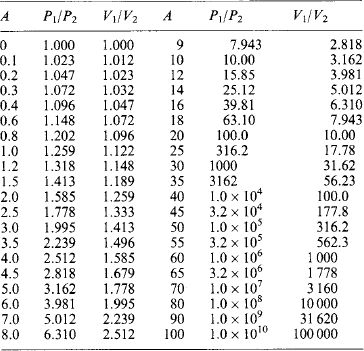
1.2.9 Power ratio
In communication networks the powers P1 and P2 at two specified points may differ widely as the result of amplification or attenuation. The power ratio P1/P2 is more convenient in logarithmic terms.
Neper [Np] This is the natural logarithm of a voltage or current ratio, given by
If the voltages are applied to, or the currents flow in, identical impedances, then the power ratio is
Decibel [dB] The power gain is given by the common logarithm lg(P1/P2) in bel [B], or most commonly by A = 10 log(P1/P2) decibel [dB]. With again the proviso that the powers are developed in identical impedances, the power gain is
Table 1.13 gives the power ratio corresponding to a gain A (in dB) and the related identical-impedance voltage (or current) ratios. Approximately, 3 dB corresponds to a power ratio of 2, and 6 dB to a power ratio of 4. The decibel equivalent of 1 Np is 8.69 dB.
1.2.10 Matrices and vectors
If a11, a12, a13, a14 … is a set of elements, then the rectangular array
arranged in m rows and n columns is called an (m × n) matrix. If m = n then A is n-square.
An ordered set of elements x = [x1, x2, x3 … xn] is called an n-vector.
An (n × 1) matrix is called a column vector and a (1 × n) matrix a row vector.
1.2.10.2 Basic operations
(i) Sum C = A+B is defined by crs = ars+brs, for r = 1 … m; s = 1 … n.
(ii) Product If A is an (m × q) matrix and B is a (q × n) matrix, then the product C = AB is an (m × n) matrix defined by (crs) = Σparpbps, p = 1 … q; r = 1 … m; s = 1 … n. If AB = BA then A and B are said to commute.
(iii) Matrix-vector product If x = [x1 … xn], then b = Ax is defined by (br) = Σparpxp,p = 1 … n; r = 1 … m.
(iv) Multiplication of a matrix by a (scalar) element If k: is an element then C = kA = Ak is defined by (crs) = k(ars).
(v) Equality If A = B, then (aij) = (bij), for i = 1 … n; j = 1 … m.
1.2.10.3 Rules of operation
(i) Associativity A+(B+C) = (A+B)+C, A(BC) = (AB)C = ABC.
(ii) Distributivity A(B+C) = AB+AC, (B+C)A = BA+CA.
(iii) Identity If U is the (n × n) matrix (δij), i, j = 1 … n, where δij = 1 if i = j and 0 otherwise, then U is the diagonal unit matrix and A U = A.
(iv) Inverse If the product U = AB exists, then B = A−1 the inverse matrix of A. If both inverses A−1 and B−1 exist, then (A B)−1 = B−1 A−1.
(v) Transposition The transpose of A is written as AT and is the matrix whose rows are the columns of A. If the product C = AB exists then CT = (AB)T = BTAT
(vi) Conjugate For A = (ars), the congugate of A is denoted by A* = (ars*).
1.2.10.4 Determinant and trace
(i) The determinant of a square matrix A denoted by |A|, also det(A), is defined by the recursive formula |A|=a11 M11 − a12 M12+a13 M13 … (-1)na1n M1n where M11 is the determinant of the matrix with row 1 and column 1 missing, M12 is the determinant of the matrix with row 1 and column 2 missing etc.
(ii) The Trace of A is denoted by tr(A) = Σi aii, i = 1, 2 … n.
(iii) Singularity The square matrix A is singular if det (A) = 0.
1.2.10.5 Eigensystems
(i) Eigenvalues The eigenvalues of a matrix λ(A) are the n complex roots λ1(A), λ2(A) … λn(A) of the characteristic polynomial det(A − λU) = 0. Normally in most engineering systems there are no equal roots so the eigenvalues are distinct.
(ii) Eigenvectors For any distinct eigenvalue λi (A), there is an associated non-zero right eigenvector Xi satisfying the homogeneous equations (A − λiU) Xi = 0, i = 1, 2 … n. The matrix (A − λiU) is singular, however, because the det (A − λiU) = 0; hence Xi is not unique. In each set of equations (A − λiU) Xi = 0 one equation is redundant and only the relative values of the elements of Xi can be determined. Thus the eigenvectors can be scaled arbitrarily, one element being assigned a value and the other elements determined accordingly from the remaining non-homogeneous equations.
The equations can be written also as AXi = λiXi, or combining all eigenvalues and right eigenvectors, AX = ΛX, where Λ is a diagonal matrix of the eigenvalues and X is a square matrix containing all the right eigenvectors in corresponding order.
Since the eigenvalues of A and AT are identical, for every eigenvalue λi associated with an eigenvector Xi of A there is also an eigenvector Pi of AT such that ATPi = λiPi. Alternatively the eigenvector Pi can be considered to be the left eigenvector of A by transposing the equation to give ![]() , or combining into one matrix equation, PTA = PTΛ.
, or combining into one matrix equation, PTA = PTΛ.
Reciprocal eigenvectors Post-multiplying this last equation by the right eigenvector matrix X gives PTA X = PTΛX, which summarises the n sets of equations ![]() , where ki is a scalar formed from the (1 × n) by (n × 1) vector product
, where ki is a scalar formed from the (1 × n) by (n × 1) vector product ![]() . With both Pi and Xi being scaled arbitrarily, re-scaling the left eigenvectors such that Wi = (1/ki) Pi, gives
. With both Pi and Xi being scaled arbitrarily, re-scaling the left eigenvectors such that Wi = (1/ki) Pi, gives ![]() , if i = j, and = 0 otherwise. In matrix form WT X = U, the unit matrix. The re-scaled left eigenvectors
, if i = j, and = 0 otherwise. In matrix form WT X = U, the unit matrix. The re-scaled left eigenvectors ![]() are said to be the reciprocal eigenvectors corresponding to the right eigenvectors Xi.
are said to be the reciprocal eigenvectors corresponding to the right eigenvectors Xi.
(iii) Eigenvalue sensitivity analysis The change in the numerical value of λi with a change in any matrix A element δars is to a first approximation given by δλi = (wr)i (xs)i δars where (wr)i is the r-th element of the reciprocal eignvector Wi corresponding to λi and (xs)i is the s-th element of the associated right eigenvector Xi. In more compact form the sensitivity coefficients δλi/δars or condition numbers of all n eigenvalues with respect to all elements of matrix A are expressible by the 1-term dyads ![]() .
.

The matrix Si is known as i-th eigenvalue sensitivity matrix.
(iv) Matrix functions Transposed eigenvalue sensitivity matrices appear also in the dyadic expansion of a matrix and in matrix functions, thus ![]() . Likewise
. Likewise ![]() or in general
or in general ![]() ; thus, for example,
; thus, for example, ![]() .
.
1.2.10.6 Norms
(i) Vector norms A scalar measure of the magnitude of a vector X with elements x1, x2 … xn, is provided by a norm, the general family of norms being defined by ||X|| = [Σi |xi|p]1/p. The usual norms are found from the values of p. If p = 1, ||X|| is the sum of the magnitudes of the elements, p = 2, ||X|| is Euclidean norm or square root of the sum of the squares of the magnitudes of the elements,
p = infinity, ||X|| is the infinity norm or magnitude of the largest element.
(ii) Matrix norms Several norms for matrices have also been defined, for matrix A two being the Euclidean norm, ||A||E = [ΣrΣs|ars|2]1/2, r = 1, 2 … m; s = 1, 2 … n, and the absolute norm, ||A|| = maxr, s |ars|.
1.3 Physical quantities
Engineering processes involve energy associated with physical materials to convert, transport or radiate energy. As energy has several natural forms, and as materials differ profoundly in their physical characteristics, separate technologies have been devised around specific processes; and materials may have to be considered macroscopically in bulk, or in microstructure (molecular, atomic and subatomic) in accordance with the applications or processes concerned.
1.3.1 Energy
Like ‘force’ and ‘time’, energy is a unifying concept invented to systematise physical phenomena. It almost defies precise definition, but may be described, as an aid to an intuitive appreciation.
Energy is the capacity for ‘action’ or work.
Work is the measure of the change in energy state.
State is the measure of the energy condition of a system.
System is the ordered arrangement of related physical entities or processes, represented by a model.
Mode is a description or mathematical formulation of the system to determine its behaviour.
Behaviour describes (verbally or mathematically) the energy processes involved in changes of state. Energy storage occurs if the work done on a system is recoverable in its original form. Energy conversion takes place when related changes of state concern energy in a different form, the process sometimes being reversible. Energy dissipation is an irreversible conversion into heat. Energy transmission and radiation are forms of energy transport in which there is a finite propagation time.
In a physical system there is an identifiable energy input Wi and output Wo. The system itself may store energy Ws and dissipate energy W. The energy conservation principle states that
Comparable statements can be made for energy changes Δw and for energy rates (i.e. powers), giving
1.3.1.1 Analogues
In some cases the mathematical formulation of a system model resembles that of a model in a completely different physical system: the two systems are then analogues. Consider linear and rotary displacements in a simple mechanical system with the conditions in an electric circuit, with the following nomenclature:
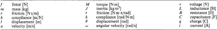
The force necessary to maintain a uniform linear velocity u against a viscous frictional resistance r is f = ur; the power is p = fu = u2r and the energy expended over a distance l is W = fut = u2rt, since l = ut. These are, respectively, the analogues of v = iR, p = vi = i2R and W = vit = i2Rt for the corresponding electrical system. For a constant angular velocity in a rotary mechanical system, M = ωr, p = Mω = ω2r and W = ω2rt, since θ = ωt.
If a mass is given an acceleration du/dt, the force required is f = m(du/dt) and the stored kinetic energy at velocity u1 is ![]() . For rotary acceleration, M = J(dω/dt) and
. For rotary acceleration, M = J(dω/dt) and ![]() . Analogously the application of a voltage v to a pure inductor L produces an increase of current at the rate di/dt such that v = L(di/dt) and the magnetic energy stored at current i1 is
. Analogously the application of a voltage v to a pure inductor L produces an increase of current at the rate di/dt such that v = L(di/dt) and the magnetic energy stored at current i1 is ![]() .
.
A mechanical element (such as a spring) of compliance k (which describes the displacement per unit force and is the inverse of the stiffness) has a displacement l = kf when a force f is applied. At a final force f1 the potential energy stored is ![]() . For the rotary case, θ = kM and
. For the rotary case, θ = kM and ![]() . In the electric circuit with a pure capacitance C, to which a p.d. v is applied, the charge is q = Cv and the electric energy stored at v1 is
. In the electric circuit with a pure capacitance C, to which a p.d. v is applied, the charge is q = Cv and the electric energy stored at v1 is ![]() .
.
Use is made of these correspondences in mechanical problems (e.g. of vibration) when the parameters can be considered to be ‘lumped’. An ideal transformer, in which the primary m.m.f. in ampere-turns i1N1 is equal to the secondary m.m.f. i2N2 has as analogue the simple lever, in which a force f1 at a point distant l1 from the fulcrum corresponds to f2 at l2 such that f1l1 = f2l2.
A simple series circuit is described by the equation v = L(di/dt)+Ri+q/C or, with i written as dq/dt,
A corresponding mechanical system of mass, compliance and viscous friction (proportional to velocity) in which for a displacement l the inertial force is m(du/dt), the compliance force is l/k and the friction force is ru, has a total force
Thus the two systems are expressed in identical mathematical form.
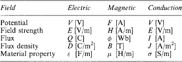
1.3.1.2 Fields
Several physical problems are concerned with ‘fields’ having stream-line properties. The eddyless flow of a liquid, the current in a conducting medium, the flow of heat from a high- to a low-temperature region, are fields in which representative lines can be drawn to indicate at any point the direction of the flow there. Other lines, orthogonal to the flow lines, connect points in the field having equal potential. Along these equipotential lines there is no tendency for flow to take place.
Static electric fields between charged conductors (having equipotential surfaces) are of interest in problems of insulation stressing. Magnetic fields, which in air-gaps may be assumed to cross between high-permeability ferromagnetic surfaces that are substantially equipotentials, may be studied in the course of investigations into flux distribution in machines. All the fields mentioned above satisfy Laplacian equations of the form
The solution for a physical field of given geometry will apply to other Laplacian fields of similar geometry, e.g.
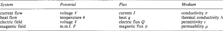
The ratio I/V for the first system would give the effective conductance G; correspondingly for the other systems, q/θ gives the thermal conductance, Q/V gives the capacitance and Φ/F gives the permeance, so that if measurements are made in one system the results are applicable to all the others.
It is usual to treat problems as two-dimensional where possible. Several field-mapping techniques have been devised, generally electrical because of the greater convenience and precision of electrical measurements. For two-dimensional problems, conductive methods include high-resistivity paper sheers, square-mesh ‘nets’ of resistors and electrolytic tanks. The tank is especially adaptable to three-dimensional cases of axial symmetry.
In the electrolytic tank a weak electrolyte, such as ordinary tap-water, provides the conducting medium. A scale model of the electrode system is set into the liquid. A low-voltage supply at some frequency between 50 Hz and 1 kHz is connected to the electrodes so that current flows through the electrolyte between them. A probe, adjustable in the horizontal plane and with its tip dipping vertically into the electrolyte, enables the potential field to be plotted. Electrode models are constructed from some suitable insulant (wood, paraffin wax, Bakelite, etc.), the electrode outlines being defined by a highly conductive material such as brass or copper. The metal is silver-plated to improve conductivity and reduce polarisation. Three-dimensional cases with axial symmetry are simulated by tilting the tank and using the surface of the electrolyte as a radial plane of the system.
The conducting-sheet analogue substitutes a sheet of resistive material (usually ‘teledeltos’ paper with silver-painted electrodes) for the electrolyte. The method is not readily adaptable to three-dimensional plots, but is quick and inexpensive in time and material.
The mesh or resistor-net analogue replaces a conductive continuum by a square mesh of equal resistors, the potential measurements being made at the nodes. Where the boundaries are simple, and where the ‘grain size’ is sufficiently small, good results are obtained. As there are no polarisation troubles, direct voltage supply can be used. If the resistors are made adjustable, the net can be adapted to cases of inhomogeneity, as when plotting a magnetic field in which permeability is dependent on flux density. Three-dimensional plots are made by arranging plane meshes in layers; the nodes are now the junctions of six instead of four resistors.
A stretched elastic membrane, depressed or elevated in appropriate regions, will accommodate itself smoothly to the differences in level: the height of the membrane everywhere can be shown to be in conformity with a two-dimensional Laplace equation. Using a rubber sheet as a membrane, the path of electrons in an electric field between electrodes in a vacuum can be investigated by the analogous paths of rolling bearing-balls. Many other useful analogues have been devised, some for the rapid solution of mathematical processes.
Recently considerable development has been made in point-by-point computer solutions for the more complicated field patterns in three-dimensional space.
1.3.2 Structure of matter
Material substances, whether solid, liquid or gaseous, are conceived as composed of very large numbers of molecules. A molecule is the smallest portion of any substance which cannot be further subdivided without losing its characteristic material properties. In all states of matter molecules are in a state of rapid continuous motion. In a solid the molecules are relatively closely ‘packed’ and the molecules, although rapidly moving, maintain a fixed mean position. Attractive forces between molecules account for the tendency of the solid to retain its shape. In a liquid the molecules are less closely packed and there is a weaker cohesion between them, so that they can wander about with some freedom within the liquid, which consequently takes up the shape of the vessel in which it is contained. The molecules in a gas are still more mobile, and are relatively far apart. The cohesive force is very small, and the gas is enabled freely to contract and expand. The usual effect of heat is to increase the intensity and speed of molecular activity so that ‘collisions’ between molecules occur more often; the average spaces between the molecules increase, so that the substance attempts to expand, producing internal pressure if the expansion is resisted.
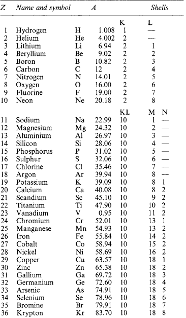
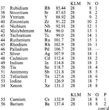
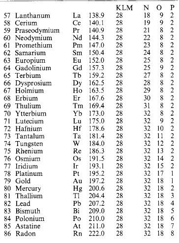
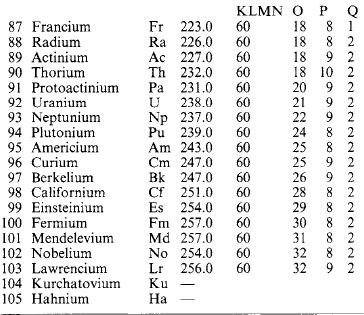
Molecules are capable of further subdivision, but the resulting particles, called atoms, no longer have the same properties as the molecules from which they came. An atom is the smallest portion of matter than can enter into chemical combination or be chemically separated, but it cannot generally maintain a separate existence except in the few special cases where a single atom forms a molecule. A molecule may consist of one, two or more (sometimes many more) atoms of various kinds. A substance whose molecules are composed entirely of atoms of the same kind is called an element. Where atoms of two or more kinds are present, the molecule is that of a chemical compound. At present over 100 elements are recognised (Table 1.14: the atomic mass number A is relative to 1/12 of the mass of an element of carbon-12).
If the element symbols are arranged in a table in ascending order of atomic number, and in columns (‘groups’) and rows (‘periods’) with due regard to associated similarities, Table 1.15: is obtained. Metallic elements are found on the left, non-metals on the right. Some of the correspondences that emerge are:
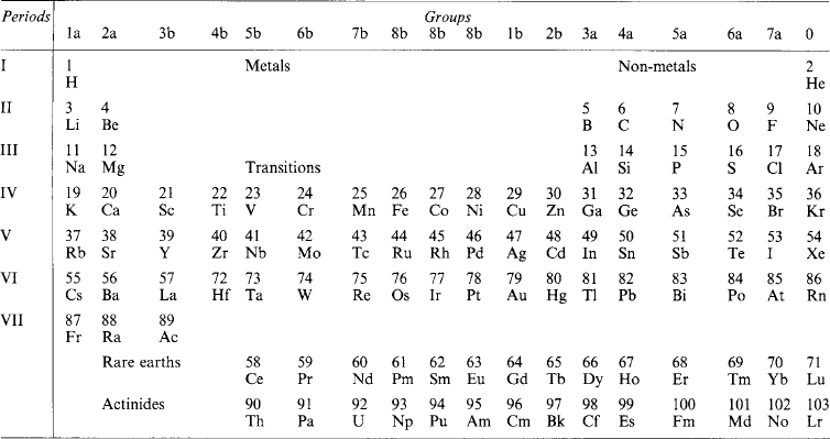
1a: Alkali metals (Li 3, Na 11, K 19, Rb 37, Cs 55, Fr 87)
2a: Alkaline earths (Be 4, Mg 12, Ca 20, Sr 38, Ba 56, Ra 88)
1b: Copper group (Cu 29, Ag 47, Au 79)
6b: Chromium group (Cr 24, Mo 42, W 74)
7a: Halogens (F 9, Cl 17, Br 35, I 53, At 85)
0: Rare gases (He 2, Ne 10, Ar 18, Kr 36, Xe 54, Rn 86)
3a–6a: Semiconductors (B 5, Si 16, Ge 32, As 33, Sb 51, Te 52)
In some cases a horizontal relation obtains as in the transition series (Sc 21 … Ni 28) and the heavy-atom rare earth and actinide series. The explanation lies in the structure of the atom.
1.3.2.1 Atomic structure
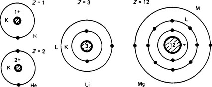
The original Bohr model of the hydrogen atom was a central nucleus containing almost the whole mass of the atom, and a single electron orbiting around it. Electrons, as small particles of negative electric charge, were discovered at the end of the nineteenth century, bringing to light the complex structure of atoms. The hydrogen nucleus is a proton, a mass having a charge equal to that of an electron, but positive. Extended to all elements, each has a nucleus comprising mass particles, some (protons) with a positive charge, others (neutrons) with no charge. The atomic mass number A is the total number of protons and neutrons in the nucleus; the atomic number Z is the number of positive charges, and the normal number of orbital electrons. The nuclear structure is not known, and the forces that bind the protons against their mutual attraction are conjectural.
The hydrogen atom (Figure 1.4) has one proton (Z = 1) and one electron in an orbit formerly called the K shell. Helium (Z = 2) has two protons, the two electrons occupying the K shell which, by the Pauli exclusion principle, cannot have more than two. The next element in order is lithium (Z = 3), the third electron in an outer L shell. With elements of increasing atomic number, the electrons are added to the L shell until it holds a maximum of 8, the surplus then occupying the M shell to a maximum of 18. The number of ‘valence’ electrons (those in the outermost shell) determines the physical and chemical properties of the element. Those with completed outer shells are ‘stable’.
Isotopes An element is often found to be a mixture of atoms with the same chemical property but different atomic masses: these are isotopes. The isotopes of an element must have the same number of electrons and protons, but differ in the number of neutrons, accounting for the non-integral average mass numbers. For example, neon comprises 90.4% of mass number 20, with 0.6% of 21 and 9.0% of mass number 22, giving a resultant mass number of 20.18.
Energy states Atoms may be in various energy states. Thus, the filament of an incadescent lamp may emit light when excited by an electric current but not when the current is switched off. Heat energy is the kinetic energy of the atoms of a heated body. The more vigorous impact of atoms may not always shift the atom as a whole, but may shift an electron from one orbit to another of higher energy level within the atom. This position is not normally stable, and the electron gives up its momentarily acquired potential energy by falling back to its original level, releasing the energy as a light quantum or photon.
Ionisation Among the electrons of an atom, those of the outermost shell are unique in that, on account of all the electron charges on the shells between them and the nucleus, they are the most loosely bound and most easily removable. In a variety of ways it is possible so to excite an atom that one of the outer electrons is torn away, leaving the atom ionised or converted for the time into an ion with an effective positive charge due to the unbalanced electrical state it has acquired. Ionisation may occur due to impact by other fast-moving particles, by irradiation with rays of suitable wavelength and by the application of intense electric fields.
1.3.2.2 Wave mechanics
The fundamental laws of optics can be explained without regard to the nature of light as an electromagnetic wave phenomenon, and photoelectricity emphasises its nature as a stream or ray of corpuscles. The phenomena of diffraction or interference can only be explained on the wave concept. Wave mechanics correlates the two apparently conflicting ideas into a wider concept of ‘waves of matter’. Electrons, atoms and even molecules participate in this duality, in that their effects appear sometimes as corpuscular, sometimes as of a wave nature. Streams of electrons behave in a corpuscular fashion in photoemission, but in certain circumstances show the diffraction effects familiar in wave action. Considerations of particle mechanics led de Broglie to write several theoretic papers (1922–1926) on the parallelism between the dynamics of a particle and geometrical optics, and suggested that it was necessary to admit that classical dynamics could not interpret phenomena involving energy quanta. Wave mechanics was established by Schrödinger in 1926 on de Broglie’s conceptions.
When electrons interact with matter, they exhibit wave properties: in the free state they act like particles. Light has a similar duality, as already noted. The hypothesis of de Broglie is that a particle of mass m and velocity u has wave properties with a wavelength λ = h/mu, where h is the Planck constant, h = 6.626 × 10⁻³⁴Js. The mass m is relativistically affected by the velocity.
When electron waves are associated with an atom, only certain fixed-energy states are possible. The electron can be raised from one state to another if it is provided, by some external stimulus such as a photon, with the necessary energy difference Δw in the form of an electromagnetic wave of wavelength λ = hc/Δw, where c is the velocity of free space radiation (3 × 10⁸m/s). Similarly, if an electron falls from a state of higher to one of lower energy, it emits energy Δw as radiation. When electrons are raised in energy level, the atom is excited, but not ionised.
1.3.2.3 Electrons in atoms
Consider the hydrogen atom. Its single electron is not located at a fixed point, but can be anywhere in a region near the nucleus with some probability. The particular region is a kind of shell or cloud, of radius depending on the electron’s energy state.
With a nucleus of atomic number Z, the Z electrons can have several possible configurations. There is a certain radial pattern of electron probability cloud distribution (or shell pattern). Each electron state gives rise to a cloud pattern, characterised by a definite energy level, and described by the series of quantum numbers n, l, ml and ms. The number n(= 1, 2, 3, …) is a measure of the energy level; l(= 0, 1, 2, …) is concerned with angular momentum; ml is a measure of the component of angular momentum in the direction of an applied magnetic field; and ms arises from the electron spin. It is customary to condense the nomenclature so that electron states corresponding to l = 0, 1, 2 and 3 are described by the letters s, p, d and f and a numerical prefix gives the value of n. Thus boron has 2 electrons at level 1 with l = 0, two at level 2 with l = 0, and one at level 3 with l = 1: this information is conveyed by the description (1s)2(2s)2(2p)1.
The energy of an atom as a whole can vary according to the electron arrangement. The most stable state is that of minimum energy, and states of higher energy content are excited. By Pauli’s exclusion principle the maximum possible number of electrons in states 1, 2, 3, 4, …, n are 2, 8, 18, 32,…, 2n2, respectively. Thus, only 2 electrons can occupy the 1s state (or K shell) and the remainder must, even for the normal minimum-energy condition, occupy other states. Hydrogen and helium, the first two elements, have, respectively, 1 and 2 electrons in the 1-quantum (K) shell; the next, lithium, has its third electron in the 2-quantum (L) shell. The passage from lithium to neon results in the filling up of this shell to its full complement of 8 electrons. During the process, the electrons first enter the 2s subgroup, then fill the 2p subgroup until it has 6 electrons, the maximum allowable by the exclusion principle (see Table 1.14:).
Very briefly, the effect of the electron-shell filling is as follows. Elements in the same chemical family have the same number of electrons in the subshell that is incompletely filled. The rare gases (He, Ne, Ar, Kr, Xe) have no uncompleted shells. Alkali metals (e.g. Na) have shells containing a single electron. The alkaline earths have two electrons in uncompleted shells. The good conductors (Ag, Cu, Au) have a single electron in the uppermost quantum state. An irregularity in the ordered sequence of filling (which holds consistently from H to Ar) begins at potassium (K) and continues to Ni, becoming again regular with Cu, and beginning a new irregularity with Rb.
The electron of a hydrogen atom, normally at level 1, can be raised to level 2 by endowing it with a particular quantity of energy most readily expressed as 10.2eV. (1 eV = 1 electron-volt = 1.6 × 10⁻¹⁹ J is the energy acquired by a free electron falling through a potential difference of 1 V, which accelerates it and gives it kinetic energy.) The 10.2V is the first excitation potential for the hydrogen atom. If the electron is given an energy of 13.6eV, it is freed from the atom, and 13.6V is the ionisation potential. Other atoms have different potentials in accordance with their atomic arrangement.
1.3.2.4 Electrons in metals
An approximation to the behaviour of metals assumes that the atoms lose their valency electrons, which are free to wander in the ionic lattice of the material to form what is called an electron gas. The sharp energy levels of the free atom are broadened into wide bands by the proximity of others. The potential within the metal is assumed to be smoothed out, and there is a sharp rise of potential at the surface which prevents the electrons from escaping: there is a potential-energy step at the surface which the electrons cannot normally overcome: it is of the order of 10 eV. If this is called W, then the energy of an electron wandering within the metals is ![]() .
.
The electrons are regarded as undergoing continual collisions on account of the thermal vibrations of the lattice, and on Fermi-Dirac statistical theory it is justifiable to treat the energy states (which are in accordance with Pauli’s principle) as forming an energy continuum. At very low temperatures the ordinary classical theory would suggest that electron energies spread over an almost zero range, but the exclusion principle makes this impossible and even at absolute zero of temperature the energies form a continuum, and physical properties will depend on how the electrons are distributed over the upper levels of this energy range.
Conductivity The interaction of free electrons with the thermal vibrations of the ionic lattice (called ‘collisions’ for brevity) causes them to ‘rebound’ with a velocity of random direction but small compared with their average velocities as particles of an electron gas. Just as a difference of electric potential causes a drift in the general motion, so a difference of temperature between two parts of a metal carries energy from the hot region to the cold, accounting for thermal conduction and for its association with electrical conductivity. The free electron theory, however, is inadequate to explain the dependence of conductivity on crystal axes in the metal.
At absolute zero of temperature (zero K = −273°C) the atoms cease to vibrate, and free electrons can pass through the lattice with little hindrance. At temperatures over the range 0.3–10 K (and usually round about 5K) the resistance of certain metals, e.g. Zn, Al, Sn, Hg and Cu, becomes substantially zero. This phenomenon, known as superconductivity, has not been satisfactorily explained.
Superconductivity is destroyed by moderate magnetic fields. It can also be destroyed if the current is large enough to produce at the surface the same critical value of magnetic field. It follows that during the superconductivity phase the current must be almost purely superficial, with a depth of penetration of the order of 10 μm.
Table 1.16
Electron emission A metal may be regarded as a potential ‘well’ of depth — V relative to its surface, so that an electron in the lowest energy state has (at absolute zero temperature) the energy W = Ve (of the order 10eV): other electrons occupy levels up to a height ε* (5–8 eV) from the bottom of the ‘well’. Before an electron can escape from the surface it must be endowed with an energy not less than φ = W − ε*, called the work function.
Emission occurs by surface irradiation (e.g. with light) of frequency v if the energy quantum hv of the radiation is at least equal to φ. The threshold of photoelectric emission is therefore with radiation at a frequency not less than v = φ/h.
Emission takes place at high temperatures if, put simply, the kinetic energy of electrons normal to the surface is great enough to jump the potential step W. This leads to an expression for the emission current i in terms of temperature T, a constant A and the thermionic work function φ:
Electron emission is also the result of the application of a high electric field intensity (of the order 1–10 GV/m) to a metal surface; also when the surface is bombarded with electrons or ions of sufficient kinetic energy, giving the effect of secondary emission.
Crystals When atoms are brought together to form a crystal, their individual sharp and well-defined energy levels merge into energy bands. These bands may overlap, or there may be gaps in the energy levels available, depending on the lattice spacing and interatomic bonding. Conduction can take place only by electron migration into an empty or partly filled band; filled bands are not available. If an electron acquires a small amount of energy from the externally applied electric field, and can move into an available empty level, it can then contribute to the conduction process.
1.3.2.5 Insulators
In this case the ‘distance’ (or energy increase Δw in electron-volts) is too large for moderate electric applied fields to endow electrons with sufficient energy, so the material remains an insulator. High temperatures, however, may result in sufficient thermal agitation to permit electrons to ‘jump the gap’.
1.3.2.6 Semiconductors
Intrinsic semiconductors (i.e. materials between the good conductors and the good insulators) have a small spacing of about 1 eV between their permitted bands, which affords a low conductivity, strongly dependent on temperature and of the order of one-millionth that of a conductor.
Impurity semiconductors have their low conductivity raised by the presence of minute quantities of foreign atoms (e.g. 1 in 108) or by deformations in the crystal structure. The impurities ‘donate’ electrons of energy level that can be raised into a conduction band (n-type); or they can attract an electron from a filled band to leave a ‘hole’, or electron deficiency, the movement of which corresponds to the movement of a positive charge (p-type).
1.3.2.7 Magnetism
Modern magnetic theory is very complex, with ramifications in several branches of physics. Magnetic phenomena are associated with moving charges. Electrons, considered as particles, are assumed to possess an axial spin, which gives them the effect of a minute current turn or of a small permanent magnet, called a Bohr magneton. The gyroscopic effect of electron spin develops a precession when a magnetic field is applied. If the precession effect exceeds the spin effect, the external applied magnetic field produces less magnetisation than it would in free space, and the material of which the electron is a constituent part is diamagnetic. If the spin effect exceeds that due to precession, the material is paramagnetic. The spin effect may, in certain cases, be very large, and high magnetisations are produced by an external field: such materials are ferromagnetic.
Table 1.19
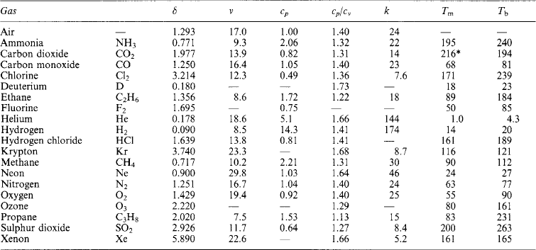
Values at 0°C (273 K) and atmospheric pressure:
cp specific heat capacity [kJ/(kg K)]
cp/cv ratio between specific neat capacity at constant pressure and at constant volume
*At pressure of 5 atm.
An iron atom has, in the n = 4 shell (N), electrons that give it conductive properties. The K, L and N shells have equal numbers of electrons possessing opposite spin directions, so cancelling. But shell M contains 9 electrons spinning in one direction and 5 in the other, leaving 4 net magnetons. Cobalt has 3, and nickel 2. In a solid metal further cancellation occurs and the average number of unbalanced magnetons is: Fe, 2.2; Co, 1.7; Ni, 0.6.
In an iron crystal the magnetic axes of the atoms are aligned, unless upset by excessive thermal agitation. (At 770°C for Fe, the Curie point, the directions become random and ferromagnetism is lost.) A single Fe crystal magnetises most easily along a cube edge of the structure. It does not exhibit spontaneous magnetisation like a permanent magnet, however, because a crystal is divided into a large number of domains in which the various magnetic directions of the atoms form closed paths. But if a crystal is exposed to an external applied magnetic field, (a) the electron spin axes remain initially unchanged, but those domains having axes in the favourable direction grow at the expense of the others (domain wall displacement); and (b) for higher field intensities the spin axes orientate into the direction of the applied field.
If wall movement makes a domain acquire more internal energy, then the movement will relax again when the external field is removed. But if wall movement results in loss of energy, the movement is non-reversible—i.e. it needs external force to reverse it. This accounts for hysteresis and remanence phenomena.
Table 1.20
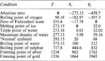
Temperature T[kelvin] corresponds to θc = T − 273.15 [degree Celsius] and to θf = θc (9/5)–32 [degree Fahrenheit].
The closed-circuit self-magnetisation of a domain gives it a mechanical strain. When the magnetisation directions of individual domains are changed by an external field, the strain directions alter too, so that an assembly of domains will tend to lengthen or shorten. Thus, readjustments in the crystal lattice occur, with deformations (e.g. 20 parts in 106) in one direction. This is the phenomenon of magnetostriction.
The practical art of magnetics consists in control of magnetic properties by alloying, heat treatment and mechanical working to produce variants of crystal structure and consequent magnetic characteristics.
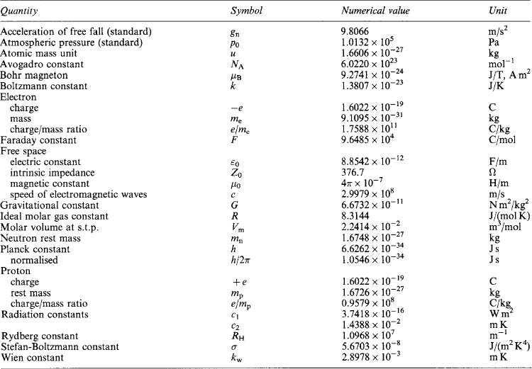
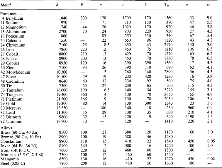
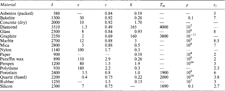
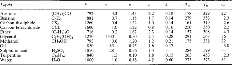
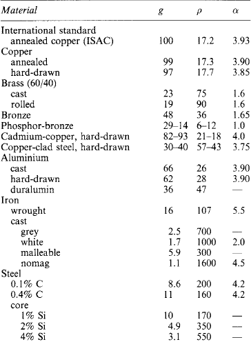
1.4 Physical properties
The nature, characteristics and properties of materials arise from their atomic and molecular structure. Tables of approximate values for the physical properties of metals, non-metals, liquids and gases are appended, together with some characteristic temperatures and the numerical values of general physical constants.
1.5 Electricity
In the following paragraphs electrical phenomena are described in terms of the effects of electric charge, at a level adequate for the purpose of simple explanation.
In general, charges may be at rest, or in motion, or in acceleration. At rest, charges have around them an electric (or electrostatic) field of force. In motion they constitute a current, which is associated with a magnetic (or electrodynamic) field of force additional to the electric field. In acceleration, a third field component is developed which results in energy propagation by electromagnetic waves.
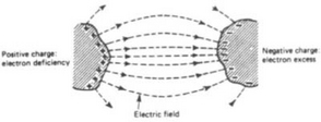
1.5.1 Charges at rest
Figure 1.5 shows two bodies in air, charged by applying between them a potential difference, or (having been in close contact) by forcibly separating them. Work must have been done in a physical sense to produce on one an excess and on the other a deficiency of electrons, so that the system is a repository of potential energy. (The work done in separating charges is measured by the product of the charges separated and the difference of electrical potential that results.) Observation of the system shows certain effects of interest: (1) there is a difference of electric potential between the bodies depending on the amount of charge and the geometry of the system; (2) there is a mechanical force of attraction between the bodies. These effects are deemed to be manifestations of the electric field between the bodies, described as a special state of space and depicted by lines of force which express in a pictorial way the strength and direction of the force effects. The lines stretch between positive and negative elements of charge through the medium (in this case, air) which separates the two charged bodies. The electric field is only a concept—for the lines have no real existence—used to calculate various effects produced when charges are separated by any method which results in excess and deficiency states of atoms by electron transfer. Electrons and protons, or electrons and positively ionised atoms, attract each other, and the stability of the atom may be considered due to the balance of these attractions and dynamic forces such as electron spin. Electrons are repelled by electrons and protons by protons, these forces being summarised in the rules, formulated experimentally long before our present knowledge of atomic structure, that ‘like charges repel and unlike charges attract one another’.
1.5.2 Charges in motion
In substances called conductors, the outer shell electrons can be more or less freely interchanged between atoms.
In copper, for example, the molecules are held together comparatively rigidly in the form of a ‘lattice’—which gives the piece of copper its permanent shape—through the interstices of which outer electrons from the atoms can be interchanged within the confines of the surface of the piece, producing a random movement of free electrons called an ‘electron atmosphere’. Such electrons are responsible for the phenomenon of electrical conductivity.
In other substances called insulators, all the electrons are more or less firmly bound to their parent atoms, so that little or no relative interchange of electron charges is possible. There is no marked line of demarcation between conductors and insulators, but the copper group metals, in the order silver, copper, gold, are outstanding in the series of conductors.
1.5.2.1 Conduction
Conduction is the name given to the movement of electrons, or ions, or both, giving rise to the phenomena described by the term electric current. The effects of a current include a redistribution of charges, heating of conductors, chemical changes in liquid solutions, magnetic effects, and many subsidiary phenomena.
If at a specified point on a conductor (Figure 1.6) n1 carriers of electric charge (they can be water-drops, ions, dust particles, etc.) each with a positive charge e1 arrive per second, and n2 carriers (such as electrons) each with a negative charge e2 arrive in the opposite direction per second, the total rate of passing of charge is n1e1+n2e2, which is the charge per second or current. A study of conduction concerns the kind of carriers and their behaviour under given conditions. Since an electric field exerts mechanical forces on charges, the application of an electric field (i.e. a potential difference) between two points on a conductor will cause the movement of charges to occur, i.e. a current to flow, so long as the electric field is maintained.
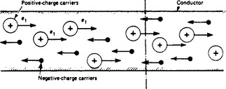
The discontinuous particle nature of current flow is an observable factor. The current carried by a number of electricity carriers will vary slightly from instant to instant with the number of carriers passing a given point in a conductor. Since the electron charge is 1.6 × 10⁻¹⁹ C, and the passage of one coulomb per second (a rate of flow of one ampere) corresponds to 1019/1.6 = 6.3 × 10¹⁸ electron charges per second, it follows that the discontinuity will be observed only when the flow comprises the very rapid movement of a few electrons. This may happen in gaseous conductors, but in metallic conductors the flow is the very slow drift (measurable in mm/s) of an immense number of electrons.
A current may be the result of a two-way movement of positive and negative particles. Conventionally the direction of current flow is taken as the same as that of the positive charges and against that of the negative ones.
1.5.2.2 Metals
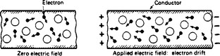
Reference has been made above to the ‘electron atmosphere’ of electrons in random motion within a lattice of comparatively rigid molecular structure in the case of copper, which is typical of the class of good metallic conductors. The random electronic motion, which intensifies with rise in temperature, merges into an average shift of charge of almost (but not quite) zero continuously (Figure 1.7). When an electric field is applied along the length of a conductor (as by maintaining a potential difference across its ends), the electrons have a drift towards the positive end superimposed upon their random digressions. The drift is slow, but such great numbers of electrons may be involved that very large currents, entirely due to electron drift, can be produced by this means. In their passage the electrons are impeded by the molecular lattice, the collisions producing heat and the opposition called resistance. The conventional direction of current flow is actually opposite to that of the drift of charge, which is exclusively electronic.
1.5.2.3 Liquids
Liquids are classified according to whether they are non-electrolytes (non-conducting) or electrolytes (conducting). In the former the substances in solution break up into electrically balanced groups, whereas in the latter the substances form ions, each a part of a single molecule with either a positive or a negative charge. Thus, common salt, NaCl, in a weak aqueous solution breaks up into sodium and chlorine ions. The sodium ion Na+ is a sodium atom less one electron; the chlorine ion Cl− is a chlorine atom with one electron more than normal. The ions attach themselves to groups of water molecules. When an electric field is applied, the sets of ions move in opposite directions, and since they are much more massive than electrons, the conductivity produced is markedly inferior to that in metals. Chemical actions take place in the liquid and at the electrodes when current passes. Faraday’s Electrolysis Law states that the mass of an ion deposited at an electrode by electrolyte action is proportional to the quantity of electricity which passes and to the chemical equivalent of the ion.
1.5.2.4 Gases
Gaseous conduction is strongly affected by the pressure of the gas. At pressures corresponding to a few centimetres of mercury gauge, conduction takes place by the movement of positive and negative ions. Some degree of ionisation is always present due to stray radiations (light, etc.). The electrons produced attach themselves to gas atoms and the sets of positive and negative ions drift in opposite directions. At very low gas pressures the electrons produced by ionisation have a much longer free path before they collide with a molecule, and so have scope to attain high velocities. Their motional energy may be enough to shockionise neutral atoms, resulting in a great enrichment of the electron stream and an increased current flow. The current may build up to high values if the effect becomes cumulative, and eventually conduction may be effected through a spark or arc.
In a vacuum conduction can be considered as purely electronic, in that any electrons present (there can be no molecular matter present in a perfect vacuum) are moved in accordance with the force exerted on them by an applied electric field. The number of electrons is small, and although high speeds may be reached, the conduction is generally measurable only in milli- or microamperes.
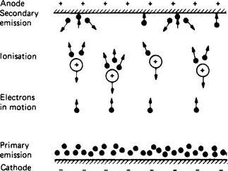
Some of the effects are illustrated in Figure 1.8, representing part of a vessel containing a gas or vapour at low pressure. At the bottom is an electrode, the cathode, from the surface of which electrons are emitted, generally by heating the cathode material. At the top is a second electrode, the anode, and an electric field is established between the electrodes. The field causes electrons emitted from the cathode to move upward. In their passage to the anode these electrons will encounter gas molecules. If conditions are suitable, the gas atoms are ionised, becoming in effect positive charges associated with the nuclear mass. Thereafter the current is increased by the detached electrons moving upwards and by the positive ions moving more slowly downwards. In certain devices (such as the mercury arc rectifier) the impact of ions on the cathode surface maintains its emission. The impact of electrons on the anode may be energetic enough to cause the secondary emission of electrons from the anode surface. If the gas molecules are excluded and a vacuum is established, the conduction becomes purely electronic.
1.5.2.5 Insulators
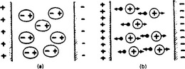
If an electric field is applied to a perfect insulator, whether solid, liquid or gaseous, the electric field affects the atoms by producing a kind of ‘stretching’ or ‘rotation’ which displaces the electrical centres of negative and positive in opposite directions. This polarisation of the dielectric insulating material may be considered as taking place in the manner indicated in Figure 1.9. Before the electric field is applied, the atoms of the insulator are neutral and unstrained; as the potential difference is raised the electric field exerts opposite mechanical forces on the negative and positive charges and the atoms become more and more highly strained (Figure 1.9(a)). On the left face the atoms will all present their negative charges at the surface: on the right face, their positive charges. These surface polarisations are such as to account for the effect known as permittivity. The small displacement of the atomic electric charges constitutes a polarisation current. Figure 1.9(b) shows that, for excessive electric field strength, conduction can take place, resulting in insulation breakdown.
The electrical properties of metallic conductors and of insulating materials are listed in Tables 1.22 and 1.23.
1.5.3 Charges in acceleration
Reference has been made to the emission of energy (photons) when an electron falls from an energy level to a lower one. Radiation has both a particle and a wave nature, the latter associated with energy propagation through empty space and through transparent media.
1.5.3.1 Maxwell equations
Faraday postulated the concept of the field to account for ‘action at a distance’ between charges and between magnets. Maxwell (1873) systematised this concept in the form of electromagnetic field equations. These refer to media in bulk. They naturally have no direct relation to the electronic nature of conduction, but deal with the fluxes of electric, magnetic and conduction fields, their flux densities, and the bulk material properties (permittivity ε, permeability μ and conductivity σ) of the media in which the fields exist. To the work of Faraday. Ampère and Gauss, Maxwell added the concept of displacement current.
Displacement current Around an electric field that changes with time there is evidence of a magnetic field. By analogy with the magnetic field around a conduction current, the rate of change of an electric field may be represented by the presence of a displacement current. The concept is applicable to an electric circuit containing a capacitor: there is a conduction current ic. in the external circuit but not between the electrodes of the capacitor. The capacitor, however, must be acquiring or losing charge and its electric field must be changing. If the rate of change is represented by a displacement current id = ic, not only is the magnetic field accounted for, but also there now exists a ‘continuity’ of current around the circuit.
Displacement current is present in any material medium, conducting or insulating, whenever there is present an electric field that changes with time. There is a displacement current along a copper conductor carrying an alternating current, but the conduction current is vastly greater even at very high frequencies. In poor conductors and in insulating materials the displacement current is comparable to (or greater than) the conduction current if the frequency is high enough. In free space and in a perfect insulator only displacement current is concerned.
Table 1.22
Electrical properties of conductors
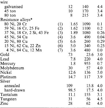
Typical approximate values at 293 K (20 °C):
*Resistance alloys: (1) furnaces, radiant elements; (2) electric irons, tubular heaters; (3) furnace elements; (4) control resistors; (5) cupro; (6) German silver, platinoid; (7) Manganin.
Equations The following symbols are used, the SI unit of each appended. The permeability and permittivity are absolute values (μ = μrμ0, ε = εrε0). Potentials and fluxes are scalar quantities: field strength and flux density, also surface and path-length elements, are vectorial.
The total electric flux emerging from a charge+Q or entering a charge −Q is equal to Q. The integral of the electric flux density D over a closed surface s enveloping the charge is
If the surface has no enclosed charge, the integral is zero. This is the Gauss law.
The magnetomotive force F, or the line integral of the magnetic field strength H around a closed path l, is equal to the current enclosed, i.e.
This is the Ampère law with the addition of displacement current.
The Faraday law states that, around any closed path l encircling a magnetic flux φ that changes with time, there is an electric field, and the line integral of the electric field strength E around the path is
Magnetic flux is a solenoidal quantity, i.e. it comprises a structure of closed loops; over any closed surface s in a magnetic field as much flux leaves the surface as enters it. The surface integral of the flux density B is therefore always zero, i.e.
To these four laws are added the constitutive equations, which relate the flux densities to the properties of the media in which the fields are established. The first two are, respectively, electric and magnetic field relations; the third relates conduction current density to the voltage gradient in a conducting medium; the fourth is a statement of the displacement current density resulting from a time rate of change of the electric flux density. The relations are
Table 1.23
Electrical properties of insulating materials Typical approximate values (see also Section 1.4):
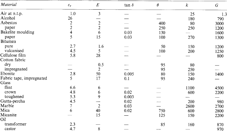
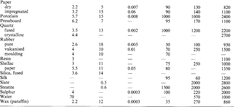
Typical approximate (see also Section 1.4):
In electrotechnology concerned with direct or low-frequency currents, the Maxwell equations are rarely used in the form given above. Equation (1.2), for example, appears as the number of amperes (or ampere-turns) required to produce in an area a the specified magnetic flux φ = Ba = μHa. Equation (1.3) in the form e = −(dφ/dt) gives the e.m.f. in a transformer primary or secondary turn. The concept of the ‘magnetic circuit’ embodies Equation (1.4). But when dealing with such field phenomena as the eddy currents in massive conductors, radio propagation or the transfer of energy along a transmission line, the Maxwell equations are the basis of analysis.
1.5.3.2 Electromagnetic wave
The local ‘induction’ field of a charge at rest surrounds it in a predictable pattern. Let the position of the charge be suddenly displaced. The field pattern also moves, but because of the finite rate of propagation there will be a region in which the original field has not yet been supplanted by the new. At the instantaneous boundary the electric field pattern may be pictured as ‘kinked’, giving a transverse electric field component that travels away from the charge. Energy is propagated, because the transverse electric field is accompanied by an associated transverse magnetic field in accordance with the Ampère law.
Consider a unit cube of free space (Figure 1.10) approached by a transverse electric field of strength E at a velocity u in the specified direction. As E enters the cube, it produces therein an electric flux, of density D = ε0E increasing at the rate Du. This is a displacement current which produces a magnetic field of strength H and flux density B = μ0H increasing at the rate Bu. Then the E and H waves are mutually dependent:
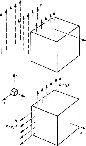
Multiplication and division of (1.5) and (1.6) give
The velocity of propagation in free space is thus fixed; the ratio E/H is also fixed, and is called the intrinsic impedance. Further, ![]() , showing that the electric and magnetic energy densities are equal.
, showing that the electric and magnetic energy densities are equal.
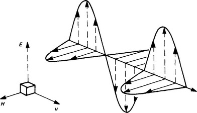
Propagation is normally maintained by charge acceleration which results from a high-frequency alternating current (e.g. in an aerial), so that waves of E and H of sinusoidal distribution are propagated with a wavelength dependent on the frequency (Figure 1.11). There is a fixed relation between the directions of E, H and the energy flow. The rate at which energy passes a fixed point is EH[W/m2], and the direction of E is taken as that of the wave polarisation.
Plane wave transmission in a perfect homogeneous loss-free insulator takes place as in free space, except that ε0 is replaced by ε = εrε0, where εr is the relative permittivity of the medium: the result is that both the propagation velocity and the intrinsic impedance are reduced.
When a plane wave from free space enters a material with conducting properties, it is subject to attenuation by reason of the I2R loss. In the limit, a perfect conductor presents to the incident wave a complete barrier, reflecting the wave as a perfect mirror. A wave incident upon a general medium is partly reflected, and partly transmitted with attenuation and phase-change.
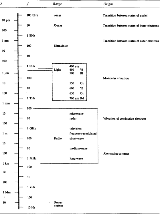
Table 1.24: gives the wavelength and frequency of free space electromagnetic waves with an indication of their technological range and of the physical origin concerned.