Chapter 8
Evaluating Environmental Performance During Process Synthesis
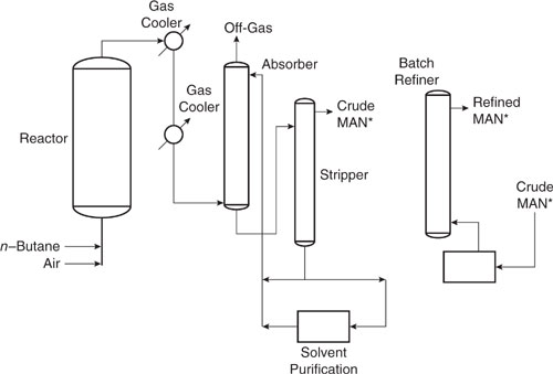
The design of chemical processes proceeds through a series of steps, beginning with the specification of the input-output structure of the process and concluding with a fully specified flowsheet. Traditionally, environmental performance has only been evaluated at the final design stages, when the process is fully specified. This chapter presents methodologies that can be employed at a variety of stages in the design process, allowing the process engineer more flexibility in choosing design options that improve environmental performance.
8.1 Introduction
The search for “greener chemistry,” described in the previous chapter, can lead to many exciting developments. New, simpler synthesis pathways could be discovered for complex chemical products, resulting in a process that generates less toxic byproducts and lowers the overall risk associated with the process. Toxic intermediates used in the synthesis of commodity chemicals might be eliminated. Benign solvents might replace more environmentally hazardous materials. However, these developments will involve new chemical processes as well as Green Chemistry.
The art and craft of creating chemical processes is the topic of a number of excellent textbooks (see, for example, Douglas, 1988). A fundamental theme that arises in each of these texts is that the design process proceeds through a series of steps, each involving an evaluation of the process performance. At the earliest stages of a design, only the most basic features of a process are proposed. These include the raw materials and chemical pathway to be used, as well as the overall material balances for the major products, byproducts, and raw materials. Large numbers of design alternatives are screened at this early design stage, and the screening tools used to evaluate the alternatives must be able to handle efficiently large numbers of alternative design concepts. As design concepts are screened, a select few might merit further study. Preliminary designs for the major pieces of equipment to be used in the process need to be specified for the design options that merit further study. Material flows for both major and minor byproducts are estimated. Rough emission estimates, based on analogous processes, might be considered. At this development stage, where fewer design alternatives are considered, more effort can be expended in evaluating each design alternative, and more information is available to perform the evaluation. If a design alternative appears attractive at this stage, a small-scale pilot plant of the process might be constructed and a detailed process flow sheet for a full-scale process might be constructed. Very few new design ideas reach this stage, and the investments made in evaluating design alternatives at this level are substantial. Therefore, process evaluation and screening tools can be quite sophisticated.
Traditionally, evaluations of environmental performance have been restricted to the last stages of this engineering design process, when most of the critical design decisions have already been made. A better approach would be to evaluate environmental performance at each step in the design process. This would require, however, a hierarchy of tools for evaluating environmental performance. Tools that can be efficiently applied to large numbers of alternatives, using limited information, are necessary for evaluating environmental performance at the earliest design stages. More detailed tools could be employed at the development stages, where potential emissions and wastes have been identified. Finally, detailed environmental impact assessments would be performed as a process nears implementation.
This chapter and Chapter 11 present a hierarchy of tools for evaluating the environmental performance of chemical processes. Three tiers of environmental performance tools will be presented. The first tier of tools, presented in Section 8.2, is appropriate for situations where only chemical structures and the input-output structure of a process is known. Section 8.3 describes a second tier of tools which is appropriate for evaluating the environmental performance of preliminary process designs. This tier includes tools for estimating wastes and emissions. Finally, Section 8.4 introduces methods for the detailed evaluation of flowsheet alternatives, which will be discussed in Chapter 11.
8.2 Tier 1 Environmental Performance Tools
At the earliest stages of a process design, only the most elementary data on raw materials, products, and byproducts of a chemical process may be available and large numbers of design alternatives may need to be considered. Evaluation methods, including environmental performance evaluations, must be rapid, relatively simple, and must rely on the simplest of process material flows. This section describes methods for performing environmental evaluations at this level.
8.2.1 Economic Criteria
As a simple example, consider two alternative processes for the manufacture of methyl methacrylate. Billions of pounds of methyl methacrylate are manufactured annually. Methyl methacrylate can be manufactured through an acetone-cyanohydrin pathway:
(CH3)2C=O + HCN → HO – C(CH3)2–CN
(Acetone + hydrogen cyanide → acetone cyanohydrin)
HO–C(CH3)2–CN + H2SO4 → CH3–(C=CH2)–(C=O)–NH2(H2SO4)
(acetone cyanohydrin → methacrylamide sulfate)
The methacrylamide sulfate is then cracked, forming methacrylic acid and methylmethacrylate:
CH3–(C=CH2)–(C=O) – NH2(H2SO4) + CH3OH → CH3–(C=CH2)–(C=O)–OH → CH3–(C=CH2)–(C=O)–O–CH3
Alternatively, methyl methacrylate can be manufactured with isobutylene and oxygen as raw materials.
CH3–(C=CH2)–CH3 + O2 → CH3–(C=CH2)–(C=O)H + H2O
isobutylene + oxygen → methacrolein
CH3–(C=CH2)–(C=O)H + 0.5 O2 → CH3–(C=CH2)–(C=O)–OH
methacrolein → methacrylic acid
CH3→(C=CH2)→(C=O)→OH + CH3CH3OH → CH3→(C=CH2)→(C=O)→O→CH3 + H2O
methacrylic acid + methanol (in sulfuric acid) → methylmethacrylate
What would be an appropriate method for evaluating these alternatives for synthesizing methyl methacrylate? The first step in answering this question is to select a set of criteria to be used in the evaluation. In traditional methods of process synthesis, cost is the most common screening criterion. To evaluate alternative processes, such as the two processes used in the synthesis of methyl methacrylate, the value of the product could be compared to the cost of the raw materials. Such an evaluation would require data on the raw material input requirements, product and byproduct output, and market values of all of the materials. Approximate stoichiometric and cost data for the methyl methacrylate processes (Chang, 1996; Rudd, et al., 1981) are provided in Table 8.2-1.
Table 8.2-1 Stoichiometric and Cost Data for Two Methyl Methacrylate Synthesis Routes.
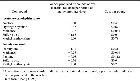
The raw material costs per pound of methyl methacrylate are simply the stoichiometric coefficients, multiplied by the cost per pound. For the first pathway, the raw material costs per pound of methyl methacrylate are:
0.68 X $0.43 + 0.32 X $0.67 + 0.37 X $0.064 + 1.63 X 0.04 = $0.60 pound of methyl methacrylate
For the isobutylene route, a similar calculation leads to a cost of $0.37 per pound of methyl methacrylate. From this simple evaluation, it is clear that the isobutylene route has lower raw material costs than the acetone-cyanohydrin route, and is probably economically preferable. It is important to note, however, that raw material costs are not the only cost factor. Different reaction pathways may lead to very different processing costs. A reaction run at high temperature or pressure may require more energy or expensive capital equipment than an alternative pathway with more expensive raw materials. Or, raw materials may be available as byproducts from other processes at a lower cost than market rates. So, simple evaluations of raw material costs should only be used in a qualitative fashion. Nevertheless, they provide a simple screening method for chemical pathways and may lead to rapid elimination of alternatives where the raw material inputs are more valuable than the products.
8.2.2 Environmental Criteria
In addition to a simple economic criterion, simple environmental criteria should be available for screening designs, based on input-output data. Selecting a single criterion or a few simple criteria that will characterize a design’s potential environmental impacts is not a simple matter. As noted elsewhere in this text, a varietyof impact categories could be considered, ranging from global warming to human health concerns. Not all of these potential impacts can be estimated effectively. Further, if only input-output data are available, there may not be sufficient information to estimate some environmental impacts. For example, estimates of global warming impacts of a design would require data on energy demands, which are often not available at this design stage.
One set of environmental criteria that can be rapidly estimated, even at the input-output level of design, are the persistence, bioaccumulation, and toxicities of the input and output materials. Chapter 5 described, in some detail, how these parameters can be estimated based on chemical structure. Consider how this might be applied to the problem of evaluating the methyl methacrylate reaction pathways. Persistence and bioaccumulation for each of the compounds listed in Table 8.2-1 are listed in Table 8.2-2.
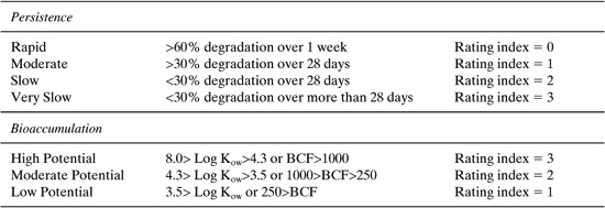
The values for persistence and bioaccumulation reported in Table 8.2-2 were calculated using the EPISUITE software package (see Appendix F), which is based on the methods described in Chapter 5. In Chapter 5, classification schemes, based on the values of persistence and bioaccumulation factors, are presented. These classifications are partially reproduced in Table 8.2-3.
Comparing these classifications to the values presented in Table 8.2-2 leads to the conclusion that none of the reactants or products in either scheme bioaccumulate or are persistent in the environment. This is a qualitative assessment. Later in this section, quantitative evaluations are discussed, and for the purposes of those quantitative assessments, the numerical ratings given in Table 8.2-3 are useful. In this case, all of the compounds would have persistence ratings of 1 and bioaccumulation ratings of 1.
Table 8.2-2 Bioaccumulation and Persistence Data for Two Synthesis Routes.
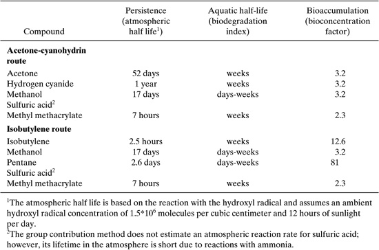
Table 8.2-3 Classification Schemes for Persistence and Bioaccumulation.
While persistence and bioaccumulation can generally be evaluated using the structure-activity methods described in Chapter 5, toxicity is more problematic. Some structure-activity relationships exist for relating chemical structures to specific human health or ecosystem health endpoints, but often the correlations are limited to specific classes of compounds. The ideal toxicity parameter would recognize a variety of potential human and ecosystem health endpoints and would be readily accessible. No such parameter exists. A variety of simple toxicity surrogates have been employed, however, including Threshold Limit Values, Permissible Exposure Limits, Recommended Exposure Limits, inhalation reference concentrations, and oral response factors. Each of these are described below.
8.2.3 Threshold Limit Values (TLVs), Permissible Exposure Limits (PELs), and Recommended Exposure Limits (RELs)
These parameters were developed to address the problem of establishing workplace limits for concentrations of chemicals. TLVs, PELs, and RELs are the estimated concentrations of chemicals that workers can be safely exposed to in occupational settings. Threshold Limit Values (TLVs), Permissible Exposure Limits (PELs), and Recommended Exposure Limits (RELs) reflect the different health impacts of chemicals and variations in exposure pathways. They are defined as follows:
Threshold Limit Value (TLV). The TLV is one type of airborne concentration limit for individual exposures in the workplace environment. The concentration is set at a level for which no adverse effects would be expected over a worker’s life-time. A number of TLVs can be cited for a chemical, depending on the length of the exposure. In this chapter, the TLVs will be time-weighted averages for an 8-hour workday and a 40-hour workweek. The concentration, again, is the level to which nearly all workers can be exposed without adverse effects. TLVs are established by a nongovernmental organization, the American Conference of Governmental Industrial Hygienists (ACGIH) (http://www.acgih.org).
Permissible Exposure Limits (PELs). The United States Occupational Safety and Health Administration (OSHA) has the legal authority to place limits on exposures to chemicals in the workplace. The workplace limits set by OSHA are referred to as PELs, and are set by OSHA in a manner similar to the setting of TLVs by ACGIH.
Recommended Exposure Limits (RELs). The National Institute for Occupational Safety and Health (NIOSH), under the Centers for Disease Control and Prevention (CDC), publishes RELs based on toxicity research. As the research complement to OSHA, NIOSH sets RELs that are intended to assist OSHA in the setting and revising of the legally binding PELs. Because no rule-making process is required for NIOSH to set RELs, these values are frequently more current than the OSHA PELs.
The TLV, PEL and REL values in Table 8.2-4 are generally quite similar, but some of the differences are worthy of comment. TLV values represent a scientific and professional assessment of hazards, while PEL values have legal implications in defining workplace conditions. Because of these legal implications, PELs are directly influenced by political, economic and feasibility issues. NIOSH, as the research complement to OSHA, is not affected by these external issues and can set their limits in a purely research environment. Because RELs do not face the same practicality issues as the PELs, NIOSH has chosen not to set safe levels of exposure for potential carcinogens, but instead recommends minimizing exposures to these substances. It is not unusual for a TLV or REL value to be established before a PEL value. Because of the greater number of chemicals for which there are reported values, there is a tendency to use TLV or REL data in screening method-ologies rather than PEL values.
One method of using TLV and PEL values to define a toxicity index is to use the inverse of the TLV (see, for example, Horvath, et al., 1995).
![]()
The concept is simple. Higher TLVs imply that higher exposures can be tolerated with no observable health effect, implying a lower health impact. A simple way to express this relationship mathematically is with an inverse relationship, as shown in Equation 8-1.
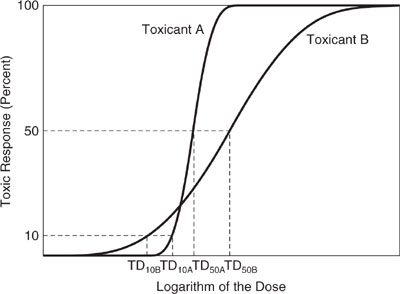
Using the TLV (or PEL, REL) as a surrogate for all toxicity impacts is a gross simplification. The TLV only accounts for direct human health effects via inhalation, and even for this purpose, it is dangerous to use the TLV as a measure of relative health impact. Figure 8.2-1 illustrates one of the pitfalls of using TLV as an indicator of relative human health impact.
Figure 8.2-1 shows the toxic response of two chemicals, A and B, as a function of dose. Chemical A has a higher threshold concentration, at which no toxic effects are observed, than chemical B. Once the threshold dose is exceeded, however, chemical A has a greater response to increasing dose than chemical B. If the TLV were based on the dose at which 10% of the population experienced health effects, then chemical B would have a lower TLV than chemical A. In contrast, if the TLV were based on the dose at which 50% of the population experienced a health impact, chemical A would have the lower TLV. So, which chemical is more toxic? The answer depends on the precise definition of toxicity and the specifics of the dose-response relationship.
Table 8.2-4 Threshold Limit Values, Permissible Exposure Limits and Recommended Exposure Limits for Selected Compounds (adapted from Crowl and Louvar, 1990. Updated with 2001 data. Note that these values continue to be periodically updated. Readers interested in current values of these parameters should consult the appropriate reference. See Appendix F.)

Figure 8.2-1 Dose response curves for two compounds that have different relative threshold limit values (TLVs), depending on how the effect level is defined (Crowl and Louvar, 1990).
This conceptual example is designed to illustrate the dangers of using simple indices as precise, quantitative indicators of environmental impacts. There is value, however, in using these simple indicators in rough, qualitative evaluations of potential environmental impacts.
8.2.4 Toxicity Weighting
An additional limitation of TLV values is that they do not consider ingestion pathways. An alternative measure of potential toxicities might incorporate both inhalation and ingestion exposure pathways. Such a system has been developed by the US EPA using data available from the EPA’s IRIS (Integrated Risk Information System) database. IRIS compiles a wide range of available data on individual compounds (http://www.epa.gov/ngispgm3/iris/subst/index.html). Three data elements that are of use in assessing potential toxicities are the inhalation reference concentration, the oral ingestion slope factor, and the unit risk. As defined in the IRIS documentation, a reference concentration is “an estimate (with uncertainty spanning perhaps an order of magnitude) of a continuous inhalation exposure to the human population (including sensitive subgroups) that is likely to be without an appreciable risk of deleterious noncancer effects during a lifetime.” The inhalation reference concentration is in some ways related to the TLV, and ratios of the TLVs of different compounds would be expected to be similar to the ratios of the inhalation reference concentrations.
An oral slope factor characterizes response to ingestion of a compound and is defined as “the slope of a dose response curve in the low dose region. When low dose linearity cannot be assumed, the slope factor is the slope of the straight line from 0 dose (and 0 excess risk) to the dose at 1% excess risk. An upper bound on this slope is usually used instead of the slope itself. The units for the slope factor are usually expressed as (mg/kg-day)-1” (US EPA, IRIS, 1999).
The unit risk is “the upper bound excess lifetime cancer risk estimated to result from continuous exposure to an agent at a concentration of 1 microgram/L in water and 1 microgram/cubic meter in air.”
A simple example may clarify the meaning of these indicators of toxicity. Consider the data available on IRIS (August, 1999) for acrylonitrile. IRIS lists acrylonitrile as a probable human carcinogen. Non-carcinogenic effects include inflammation of nasal tissues. The reference concentration for inhalation is given as 0.002 mg/m3. Lifetime exposure to this concentration is likely to be without an appreciable risk of nasal tissue inflammation and degeneration. The oral slope factor for carcinogenic risk is given as 0.54 (mg/kg-day)-1. A 100 kg person exposed to 100 mg per day would have a 0.54% excess risk. The potential individual excess lifetime cancer risk (i.e., unit risk) is 6.8 X 10⁻⁵ per microgram/m3. For a region with a population of 100,000, this corresponds to approximately 6.8 potential excess cancer cases based on a lifetime exposure of 1 microgram/m3 of acrylonitrile (i.e., an upper bound of the lifetime risk is 6.8 in 100,000). Note that 6.8 represents an upper bound and the actual risk may be much less.
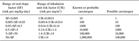
The US EPA has used data such as reference concentrations, oral slope factors, and unit risk factors to determine toxicity weighting for approximately 600 compounds reported through the Toxic Release Inventory. A complete description of the methodology and the toxicity weights are available at http://www.epa.gov/opptintr/env_ind/index.html. To briefly summarize, the EPA assembled up to four preliminary human health toxicity weights for each compound: cancer-oral, cancer-inhalation, non-cancer-oral, and non-cancer-inhalation. For each exposure pathway (oral and inhalation) the greater of the cancer and non-cancer toxicity weights was chosen. If data on only one exposure pathway were available, then the toxicity weight for that pathway was assigned to both pathways; however, if there is evidence that no exposure occurs through one of the pathways, then the toxicity weight for that pathway was assigned a value of 0.
The toxicity weights were based on the values for unit risks and slope factors. A sample of the scheme used to assign toxicity weights is given in Table 8.2-5.
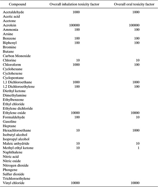
For the acrylonitrile, a probable carcinogen with an oral slope factor of 0.54, the oral toxicity weight would be 10,000. The toxicity weight for inhalation, based on a unit risk of 6.8 X 10⁻⁵ per (microgram/m3) or .068 per (milligram/m3), would be 1000. The overall toxicity weight would be based on the larger of the two values. Table 8.2-6 provides a sampling of toxicity weights. The compounds listed are the same compounds for which TLV data were listed in Table 8.2-3. The data are somewhat more sparse than the TLV data.
Table 8.2-5 Assignment of Toxicity Weights for Chemicals with Cancer Health Effects.
8.2.5 Evaluating Alternative Synthetic Pathways
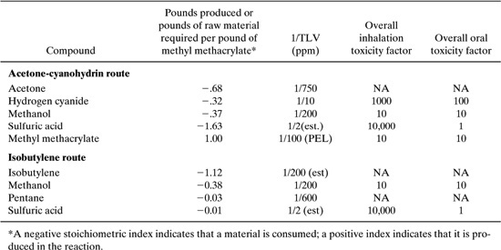
As a case study of the use of TLVs and toxicity weights in evaluating toxicity, consider once again the two routes for producing methyl methacrylate. Stoichiometric, TLV, and toxicity weight data for the two pathways are shown in Table 8.2-7.
Both the TLVs and toxicity weights in Table 8.2-7 indicate that the major health concerns associated with the two reaction pathways are due to sulfuric acid, and to a lesser extent, hydrogen cyanide.
Once these data, together with data on persistence and bioaccumulation, are known for the reactants and products, some composite index for the overall input-output structure could be established. Ideally, the index would be based on the emission rates, weighted by measures of persistence, bioaccumulation, and toxicity. In preliminary screenings, however, it is highly unlikely that detailed information will be available on emission rates. Therefore, approximations for emission rates are required. One possible approach is to use flow rate, based on stoichiometry, as a surrogate for emissions, which can then be weighted by an appropriate index.
In choosing weighting factors and an overall index for assessing environmental performance at this early stage of a design, it is important to recognize that there is no single correct choice. Many different indices have been employed. This chapter will illustrate two types of approaches that have appeared frequently in the literature. One approach is to use toxicity as a weighting factor. In this approach, the overall environmental index for a reaction is typically calculated as:
![]()
Where |νi| is the absolute value of the stoichiometric (by mass) coefficient of reactant or product i, TLVi is the threshold limit value (ppm) of reactant or product i, and the summation is taken over all reactants and products. For the acetone-cyanohydrin route:
Index = 0.68 X (1/750) + 0.32 X (1/10) + 0.37 X (1/200) + 1.63 X (1/2) + 1 X (1/100) = 0.86
For the acetone-cyanohydrin process, the index calculated using Equation 8-2 is 0.86, and for the isobutylene process, the index is 0.01, indicating a preference for the isobutylene process. This is because the indices are dominated by the contribution of sulfuric acid, which is used at a lower rate in the isobutylene process.
Table 8.2-6 Selected Toxicity Weights Drawn from the U.S. EPA’s Environmental Indicators Project.
Alternatively, the toxicity factors developed by the US EPA could be used, rather than the TLVs. In this case:
![]()
Using this approach, the index for the acetone-cyanohydrin process would be:
Index 0.68 X (0) + 0.32 (1000) + 0.37 X (10) + 1.63 X (10,000) + 1 X (10) = 16,600
For the isobutylene process, the index is 100, again indicating a preference for the isobutylene process.
Another approach that appears in preliminary environmental assessments employs persistence, bioaccumulation, and toxicity factors. Combining these factors into a composite environmental index requires that the factors be placed in a common unit system. This is generally done by assigning ratings to the persistence, bioaccumulation, and toxicity parameters. Table 8.2-2 gave rating factors for persistence and bioaccumulation for the two methyl methacrylate pathways. Ratings for human toxicity are more difficult to assign. In the evaluation of chemicals under the Toxic Substances Control Act, the US EPA employs three levels of concern for human toxicity (Wagner, et al., 1995):
• High conern
Evidence of adverse effects in human populations
Conclusive evidence of severe effects in animal studies
• Moderate concern
Suggestive animal studies
Data from close chemical analogue
Compound class known to produce toxicity
• Low concern
Chemicals that do not meet the criteria for moderate or high concern
Based on these criteria, the human toxicity concerns of the two methyl methacrylate pathways would be dominated by the concerns associated with sulfuric acid. Thus, the two pathways would have very similar levels of toxicity concern unless the relative amounts of sulfuric acid used were incorporated into the evaluation. As noted earlier, the bioaccumulation and persistence of the compounds associated with the two pathways were also identical; therefore, the overall environmental performance of the two pathways could be viewed as virtually identical.
Table 8.2-8 provides a set of three ratings for each pathway. These three ratings could be combined into a single index, or they could be retained in the matrix format shown in the table.
To summarize, the environmental performance of the two pathways for manufacturing methyl methacrylate was evaluated based on economics, toxicity, and a combined assessment of persistence, bioaccumulation, and toxicity. All of the approaches indicate a preference for the isobutylene pathway. A similar case study with a different result is given in Example 8.2-1.
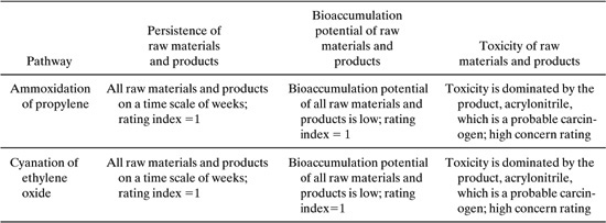
Acrylonitrile can be produced via the ammoxidation of propylene or via the cyanation of ethylene oxide. Stoichiometric, TLV, persistence, bioaccumulation, toxicity, and cost data for the two reactions are given below.
(a) Estimate the persistence and bioaccumulation potential of the two pathways
(b) Evaluate the toxicity potential of the two pathways
(c) Suggest which pathway is preferable based on environmental and economic criteria
ammoxidation of propylene:
C3H6 NH3 1.5 O2 → C3H3N 3H2O
cyanation of ethylene oxide
C2H4 + 0.5 O2 → C2H4O
C2H4O + HCN → HOC2H4CN → C3H3N + H2O
Table 8.2-8 Evaluation of Methyl Methacrylate Pathways Based on Persistence, Bioaccumulation, and Toxicity.
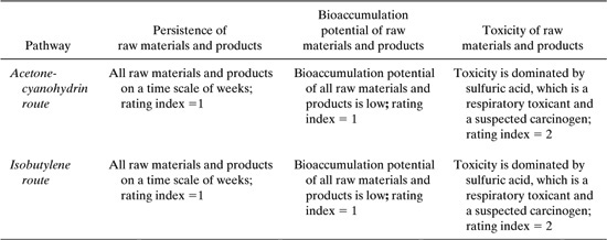
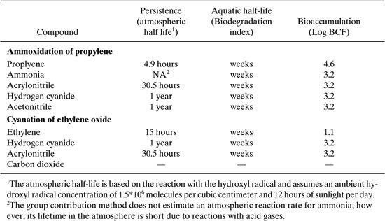
Table 8.2-9 Bioaccumulation and Persistence Data for Two Acrylonitrile Synthesis Routes.
Solution:
(a) Estimate the persistence and bioaccumulation potential of the two pathways
Based on the data in the table below, the materials used in the two pathways have comparable, relatively low persistence and bioaccumulation potentials.
The values for persistence and bioaccumulation were calculated using the EPISUITE![]() software package, which is based on the methods described in Chapter 5.
software package, which is based on the methods described in Chapter 5.
Table 8.2-10 Stoichiometric, TLV, and Toxicity Weight Data for Two Acrylonitrile Synthesis Routes.
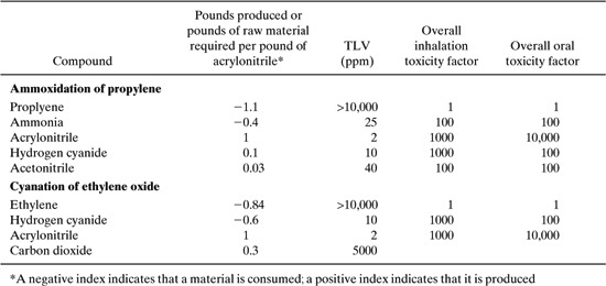
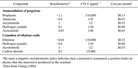
Table 8.2-11 Stoichiometric, TLV and Cost Data for Two Acrylonitrile Synthesis Routes.
(b) Evaluate the toxicity potential of the two pathways
As shown in the table and calculations below, the toxicity is dominated by the product, acrylonitrile, so the two pathways have very similar environmental performance indices.
For the acetone-cyanohydrin process, the environmental index based on the TLV and the index based on EPA’s toxicity weights are given by:
TLV Index 1.1/10,000 + 0.4/;25 + 1/2 + 0.1/10 + 0.03/40 = 0.53
EPA Index = 1.1 X 1.0 + 0.4 X 100 + 1.0 X 10,000 + 0.1 X 1,000 + 0.03 X 100 = 10,144
For the cyanation of ethylene oxide the indices are:
TLV Index 0.84/10,000 + 0.6/10 + 1/2 + 0.3/5000 = 0.56
EPA Index 0.84 X 1.0 + 0.6 X 1000 + 1.0 X 10,000 = 10,600
Based on these criteria, the human toxicity concerns of the two acrylonitrile pathways would be dominated by the concerns associated with acrylonitrile. Thus, the two pathways would have very similar levels of toxicity concern. As noted earlier, the bioaccumulation and persistence of the compounds associated with the two pathways were also identical; therefore, the overall environmental performance of the two pathways could be viewed as virtually identical.
(c) Suggest which pathway is preferable based on environmental and economic criteria
A simple economic evaluation considers the raw material costs. For the ammoxidation of propylene, the economic index is given by:
Index = 1.1 X ($0.13) + 0.4 X ($0.07) =$0.17
Table 8.2-12 Evaluation of Acrylonitrile Pathways Based on Persistence, Bioaccumulation and Toxicity.
Alternatively, an index could include raw material costs minus the value of salable byproducts:
Index = 1.1X($0.13) + 0.4X($0.07)–0.1X($0.68)–0.03X($0.65) = $0.14
For the cyanation of ethylene oxide, the economic index is:
Index = 0.84 X o.23 + 0.6 X $0.68 = $0.60
Thus, the ammoxidation of propylene is preferable to the cyanation of ethylene oxide on a cost basis; the pathways have comparable environmental characteristics.
Section 8.2 Questions For Discussion
1. What criteria would you suggest for evaluating the environmental performance of reaction pathways?
2. Can you suggest alternatives to stoichiometric coefficients for weighting environmental indices in evaluating reaction pathways?
3. What are the strengths and limitations of the environmental performance criteria described in this section?
8.3 Tier 2 Environmental Performance Tools
Once the basic input-output structure of a flow sheet is determined, a preliminary process flowsheet is developed. Typically, storage devices, reactors, and separation devices might be identified, and some information would be available about equipment sizes or process stream flow rates. This level of process specification is an appropriate time to re-examine environmental performance. At this stage of analysis, it still may be necessary to screen large numbers of design alternatives, but more information about the process is available and should be incorporated into the environmental performance evaluation. This section describes methods for performing environmental evaluations at this intermediate level. A first step in this analysis is to use the information available on the process units to estimate the magnitude and composition of emissions and wastes. Some of these emission estimation tools are described in Section 8.3.1. Once the emissions, wastes, and other process flows are characterized, any of a number of environmental performance evaluation methods can be employed. Environmental performance evaluation tools, suitable for this level of analysis, are described in Section 8.3.2.
8.3.1 Environmental Release Assessment
8.3.1.1 Basics of Releases
Releases include any spilling, leaking, pumping, pouring, emitting, emptying, discharging, injecting, escaping, leaching, dumping, or disposing into the environment (including the abandonment or discarding of containers and other closed receptacles) of any chemical or chemical mixture. The term “environment” includes water, air, and land, the three media to which release may occur. Related to releases are transfers of chemical wastes off-site for purposes other than making a salable product. Such purposes could include treatment or disposal.
8.3.1.2 Release Assessment Components
Release assessments are documents that contain information on release rates, frequencies, media of releases, and other information needed to characterize to the fullest possible extent the issues related to the releases. The audience for the document determines the amount of information about the methods used to estimate releases that should be presented. The steps required in making release assessments are:
1. Identify purpose and need for release assessment.
2. Obtain or diagram a process flowsheet.
3. Identify and list waste and emissions streams.
4. Examine the flowsheet for additional waste and emission streams.
5. For each release point identified in steps 3 and 4, determine the best available method for quantifying the release rate.
6. Determine data or information needed to use the quantification methods determined in step 5.
7. Collect data and information to fill gaps.
8. Quantify the chemical’s release rates and frequencies and the media to which releases occur.
9. Document the release assessment, including a characterization of the uncertainties in the estimates.
The purpose of the release assessment determines the information and data needed to complete the assessment. If a release assessment is to be used as part of a screening-level risk assessment, less detail and accuracy will be required than if the release assessment were being used as part of a detailed risk assessment. Knowing the purpose of the assessment can also refine the scope of the analysis. For example, if only aquatic impacts of release are of concern, then only releases to water may need to be addressed.
8.3.1.3 Process Analysis
A release assessment begins after one or more processes have been selected for analysis. At this point, the basic features (e.g., mass balances, unit operations, operating conditions) of the design are available. A flow diagram showing process streams is often a key tool in beginning the analysis.
From the flow diagram, process output streams that are not usable or salable products can be identified. List these output streams as potential releases. Often, the flowsheet does not identify other potential releases for various reasons: some are not directly attributable to process equipment, some result from process inefficiencies that are not normally considered significant, some may be infrequent, some may be difficult to quantify, and some may be overlooked. If the flowsheet development was not rigorous, many opportunities to identify potential releases, not included on the flowsheet, may exist.
Common sources of releases that are often missing in a flowsheet are:
• Fugitive emissions (including leaks, which are defined later in this section)
• Venting of equipment (e.g., breathing and displacement losses, etc.)
• Periodic equipment cleaning (may be frequent or infrequent)
• Transport container residuals (e.g., from drums, totes, tank trucks, rail cars, barges, etc.)
• Incomplete separations (e.g., distillation, gravity phase separation, filtration, etc.)
The manner in which a chemical is released is a crucial factor in assessing environmental impact. In characterizing the manner in which a chemical is released, it is convenient to first determine whether the release is expected to occur on-site or from some extension of the site to an off-site location, such as a pipe extending into a water body. On-site releases to the environment include emissions to the air, dis-charges to surface waters, and releases to land and underground injection wells. Both routine releases, such as fugitive air emissions, and accidental or non-routine releases, such as chemical spills, are part of the on-site releases. On-site releases do not include transfers or shipments of chemicals from the facility for sale or distribution in commerce, or of wastes to other facilities for disposal, treatment, energy recovery, or recycling. Chemical wastes that are transferred or shipped to an off-site location, such as a publicly owned treatment works (POTW), where the waste may be fully or partially released, are called “off-site transfers.”
Once emissions and wastes have been characterized as on-site or off-site, the on-site releases are classified by the medium or media to which the chemical is released. Releases to common classes of media are described below.
Air Releases. Releases to air (often called emissions) can be categorized into primary or secondary emissions. Primary emissions occur as a direct consequence of the production or the use within an industrial process of the compound under consideration. These primary emissions may come from either point (often called stack) or non-point (often called fugitive) sources. Stack releases of chemicals to the air occur through stacks, vents, ducts, pipes, or other confined gas streams. Stack releases include storage tank and unit operation vent emissions and, generally, air releases from air pollution control equipment. Unit operations of importance as emission sources include those which are relatively few in number within a process and are easily identifiable, such as pressure relief vents on reactors, and vents on distillation column condensers, absorption and stripping columns vents, and feed or product storage tank vents.
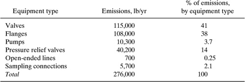
Fugitive air emissions are not releases through stacks, vents, ducts, pipes, or any other confined gas streams. These releases include fugitive equipment leaks from valves, pump seals, flanges, compressors, sampling connections, open-ended lines, etc.; releases from building ventilation systems; and any other fugitive or non-point air emissions. Fugitive emissions occur from process sources that are not easily identifiable and are of relatively large number within the process. Within a typical industrial process there may be tens to hundreds of thousands of fugitive sources (Berglund, et al., 1989).
Secondary emissions occur indirectly as a result of the production or use of a specific compound. These emission sources include utilities consumption, evaporative losses from surface impoundments and spills, and industrial wastewater collection systems.
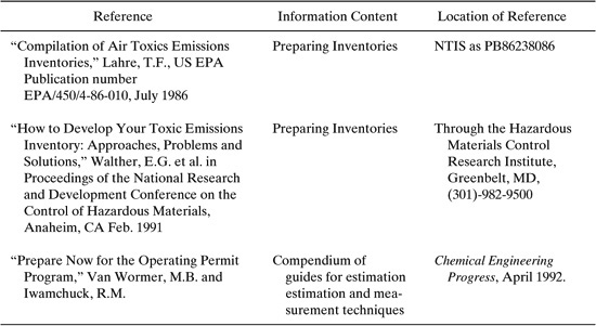
Because emissions to air can be difficult to measure and emission sources can be difficult to locate, some resources for preparing plant-wide emissions inventories have been developed. Several references for these resources are shown in Table 8.3-1.
Water Releases. Releases of chemicals from discharge points in a process can be to a receiving stream or water body. These releases include process outfalls such as pipes and open trenches, releases from on-site wastewater treatment systems, and, sometimes, the contribution from storm-water runoff. Water releases do not include discharges to a POTW or other off-site wastewater treatment facilities. These are off-site transfers.
Underground Injection Releases. Some chemicals may be injected into wells at a facility. US EPA regulations apply to underground wells, which are classified by the type of material injected into the well. The Underground Injection Control Program of the Federal Safe Drinking Water Act is found in 40 CFR Parts 144-147.
Releases to Land. Some chemicals may be released to land within the boundaries of a facility. Some facilities may have on-site landfills for chemical disposal.
Table 8.3-1 Resources for Preparing Plant-Wide Emission Inventories (Allen and Rosselot, Pollution Prevention for Chemical Processes © 1997, This material is used by permission of John Wiley & Sons, Inc.)
Land treatment/application farming is a disposal method in which a waste containing chemicals is applied onto or incorporated into soil. While this disposal method is considered a release to land, any volatilization of chemicals into the air occurring during the disposal operation is a fugitive air release.
Chemicals may also be disposed to a surface impoundment. A surface impoundment is a natural topographic depression, man-made excavation, or diked area formed primarily of earthen materials (although some may be lined with man-made materials) that is designed to hold an accumulation of liquid wastes or wastes containing free liquids. Examples of surface impoundments are holding, settling, storage, and elevation pits; ponds; and lagoons. If the pit, pond, or lagoon is intended for storage or holding without discharge, it would be considered to be a surface impoundment used as a final disposal method.
If a volatile chemical (e.g., benzene) that is in waste sent to a surface impoundment partially evaporates, that part of the release is a fugitive air emission. Chemicals released to surface impoundments that are used merely as part of a wastewater treatment process generally are not releases to land. However, if the impoundment accumulates sludges containing chemicals, this accumulation is a land release unless the sludges are removed and otherwise disposed (storage tanks are not considered to be a type of disposal).
Other land disposal includes chemicals released to land that does not fit the categories of landfills, land treatment, or surface impoundment. This other disposal would include any spills or leaks of chemicals to land.
8.3.2 Release Quantification Methods
Once the process has been analyzed to determine the points and sources of releases, the amounts of release can be estimated. These methods can be characterized and a general hierarchy of preferences can be used to determine how releases may best be quantified. The following list shows the potential methods for quantifying releases, in order, from the most preferred to the least preferred.
a. Measured release data for the chemical or indirectly measured release data using mass balance or stoichiometric ratios.
b. Release data for a surrogate chemical with similar release-affecting properties and used in the same (or very similar) process. Surrogate data may be measured, indirectly measured, modeled, or some combination of these. Some emission factors would be considered to be surrogate data.
c. Modeled release estimates:
1. Mathematically modeled (e.g., process design software, mass transfer models, etc.) release estimates for the chemical or by analogy to a surrogate chemical.
2. Rule-of-thumb release estimates, or those developed using engineering judgment.
This order of preference is expected to apply generally to most cases of release assessment. However, judgment may dictate that, in some cases, the order within the hierarchy should be changed. Examples of such a change of hierarchy order may include when data are judged to be unreliable or unrepresentative. Also, some estimates may be based on a combination of two or more of these methods. In other cases, the method used to generate some estimates may not be known due to lack of documentation (e.g., industry survey results). Judgment may also include factors such as how rigorous the modeling is in various modeling methods.
This textbook is intended to apply primarily to situations in which chemical manufacturing processes are being designed. For process design, measured release data are generally not available, requiring the use of emission factors and modeled estimates. However, for the sake of completeness, the material below will examine all methods for quantifying releases.
8.3.2.1 Measured Release Data for the Chemical
Measured release data for a chemical of interest are generally not applicable to processes in design but rather to existing processes. The following examples illustrate how data may be used to generate estimates of releases. For a continuous process, a release can be estimated by calculating the product of three measures: a chemical’s average concentration, the average volumetric flow rate of the release stream containing that chemical, and the density of the release stream. Similarly, a release could be estimated using the chemical’s weight fraction and the mass flow rate of the release stream.
Example 8.3-1
A wastewater pretreatment plant runs every day and averages 1.5 million gallons per day. The following chromium concentrations were measured. How much chromium does the POTW receive annually?
Sample Number | Cr(III) in ppm (mg/kg) |
1 | 2.7 |
2 | 0.9 |
3 | 4.1 |
4 | 3.4 |
5 | 5.1 |
6 | 2.3 |
7 | 3.8 |
Solution: The average Cr(III) concentration of the seven samples is 3.2 mg/kg. We can assume that the effluent has a density very close to that of water, 3.78 kg/gal. The average mass effluent flow is 1,500,000 gal/day effluent × 3.78 kg/gal 5,670,000 kg/day. Multiplying the average total mass daily flow by the average concentration and operating days per year yields the annual estimate: 5,670,000 kg/day effluent 3.2 kg Cr(III) / 1,000,000 kg effluent × 365 days/yr 6,600 kg/yr Cr(III).
8.3.2.2 Release Data for a Surrogate Chemical
Release data for analogous or surrogate chemicals from existing processes can sometimes be used to estimate releases of chemicals of interest either in processes in design or in existing processes. To use surrogate chemical data, similarities must exist in some physical/chemical properties of the chemicals, unit processes and their operating conditions, and quantities of chemical throughput. For instance, in Example 8.3-1, if an estimate of the release rate for Cr(VI), which is a different oxidation state of chromium than Cr(III), was desired, then Cr(III) might be used as a surrogate. If data were available indicating that a typical ratio of Cr(III) to Cr(VI) were 1000:1, then the release rate of Cr(VI) might be estimated as 1/1000 of the release rate of Cr(III).
8.3.2.3 Emission Factors
Emission factors are commonly used to estimate releases to air. A number of unit operation-specific emission factor databases have been compiled for the US EPA. For air pollutants regulated through the National Ambient Air Quality Standards (NAAQS) (SO2, NO2, CO, O3, hydrocarbons, particulates), the AP-42 compilation with supplements provides emission factors for several industrial sectors, including stationary and mobile combustion units, refuse incineration, storage tank emissions, and units in the chemical, metallurgical, minerals, food and agriculture, and wood products industries (US EPA, 1998).
The emission factors in the AP-42 database are not, in general, compoundspecific. Several databases are available from the EPA for estimating emissions of specific organic and inorganic compounds from a variety of processes in the chemical manufacturing industry. The earliest of these documents (Organic Chemical Manufacturing) is a ten-volume report which summarizes emission factors of 39 compounds for several production and use processes (US EPA, 1980). These emission factors are tabulated on a process-unit-by-process-unit basis and include reactors, separation columns, storage tanks, fugitive emission, transfer and handling operations, and wastewater treatment units. A more recent compilation of emission factors for hazardous compounds is provided in documents titled Locating and Estimating Air Emissions from Sources (L&E) (US EPA, 1998). The L&E database contains much of the data in the previously mentioned volumes of Organic Chemical Manufacturing(OCM).
The most recent and comprehensive emission factor document from the US EPA is titled the Factor Information Retrieval(FIRE) System. It contains EPA’s recommended criteria and hazardous air pollutant (HAP) emission estimation factors. The above-mentioned emission factor sources are included in the Air CHIEF CDROM available from the US EPA (US EPA, 1998). In addition to emission factors, the Air CHIEF software contains source classification codes (SCC) for over 9000 chemicals; a program to calculate controlled emissions for particulate matter (PM-2.5 and PM-10); a biogenic emission inventory system; a spreadsheet for estimating volatile organic compound (VOC) emissions from treatment, storage and disposal facility processes; and a menu-driven computer program for estimating emissions from wastewater treatment systems. (See Appendix F for more information on these resources.)
8.3.2.4 Emissions from Process Units and Fugitive Sources.
The rate of emission (E, mass/time) of VOCs from process units and operations such as reactors, distillation columns, storage tanks, transportation and handling operations, and fugitive sources can be calculated using the formula
![]()
where
mVOC is the mass fraction of the volatile organic compound in the stream or process unit
EFav (kg emitted/kg throughput) is the average emission factor ascribed to that stream or process unit
M is the mass flow rate through the unit (mass/time)
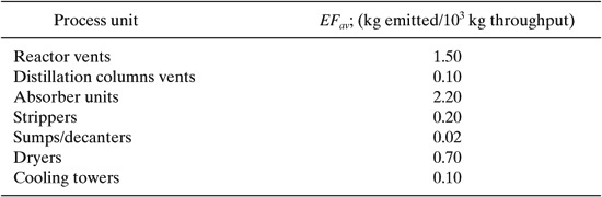
Table 8.3-2 shows average emission factors obtained from the US Environmental Protection Agency L&E database for several process units found in chemical plants.
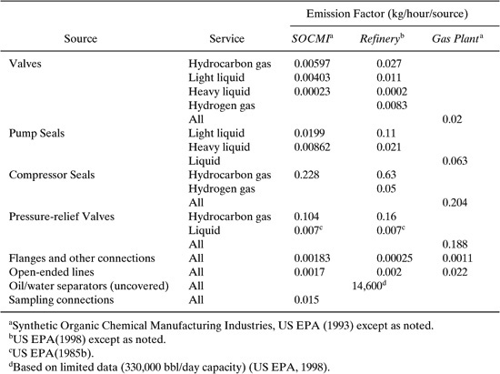
Table 8.3-3 lists the average emission factors for fugitive sources found in refineries, gas plants and synthetic organic chemical manufacturing operations.
Table 8.3-2 Average Emission Factors for Chemical Process Units Calculated from the US EPA L&E Database (Shonnard, et al. 1995).
Note that the form of the emission factors given in Table 8.3-3 is slightly different from the form shown in Equation 8-4. This is not unusual and consequently, emission factor equations should be used with care and attention to the details of units. Also note that in Table 8.3-3, liquid streams are classified into light and heavy service. A light liquid is defined as a stream in which the most volatile component present (> 20% by weight) has a vapor pressure at the stream temperature of > 0.04 lb/in2.
Table 8.3-3 Average Emission Factors for Estimating Fugitive Emissions
A company wants to sell a newly-developed substitute for dimethylsulfoxide (DMSO) in pharmaceutical manufacturing. 300,000 lb/yr of this new drop-in substitute for DMSO could be sold to two customer pharmaceutical plants that will each purchase the same volume of the substitute. US EPA requires submission of a Premanufacture Notice (PMN) for this new chemical. The PMN form requests estimated releases to all media from downstream customers (the pharmaceutical plants) in units of kg/day. Generate these estimates.
Solution: Assume that the physical/chemical properties of the new chemical match the properties of DMSO very closely. The customer plants are reluctant to divulge proprietary process information, but one detail they give is that the facilities operate five days each week for 50 weeks of the year. Based on a search of several release estimation resources, you find that the US EPA document entitled “Compilation of Air Pollutant Emission Factors” (often referred to as AP-42) contains emission factors for DMSO for the pharmaceutical industry. The reference table notes that these data are based on an industry survey. Because both the release-affecting properties and the industrial use of the new chemical and DMSO are so similar, you have concluded that these DMSO emission factors are suitable surrogates for estimating releases of your company’s new chemical. The AP-42 DMSO emission factors for the pharmaceutical industry are 1% to air emissions, 28% to sewer, and 71% to incineration (AP-42, Section 6.13). You contacted the potential customers, and they acknowledged that these AP-42 emission factors reasonably represent their facilities.
Calculation: First calculate the amount used per day at each site, then apply the emission factors to calculate the release to the media.
1. Daily average amount (mass) used at each site
300,000 lb/yr/2.20 kg/lb/2 sites/(5 days/week X 50weeks/yr) = 273 kg/day
2. Partition the daily use amount to the media based on the emission factors:
release to air = 1% of 273 kg/day = 2.7 kg/day
release to water = 28% of 273 kg/day= 76 kg/day
release to incineration =71% of 273 kg/day = 194 kg/days
Example 8.3-3
Estimate the fugitive emissions from a chemical manufacturing facility that contains 1400 valves (168 in gas service), 3048 flanges and other connectors, 27 pumps (all in liquid service), 20 pressure relief valves, and 20 sampling connections (Berglund, et al., 1989) Determine the total fugitive emissions in pounds per year using the Synthetic Organic Chemical Manufacturing Industry (SOCMI) emission factors given in Table 8.3-3. Assume that the process fluids are composed almost entirely of volatile compounds. (Allen and Rosselot, Pollution Prevention for Chemical Processes, © 1997, This material is used by permission of John Wiley & Sons, Inc.)
Solution: For the valves in gas service, the emissions are:
(168 valves) X (0.00597 kg VOC/(hr – valve))(2.2 lb/hg)(24 hr/day)(365 day/year) = 19,300 lb/yr
For the valves in light liquid service, the emissions are:
((1400 –168)valves) X (0.00403 kg VOC/(hr – valve)(2.2 lb/kg)(24 hr/day)(365 day/year)) = 95,700 lb/yr
Summing these values gives the total estimated emissions from valves, which is 115,000 lb/year. Results for the other component types are given below.
8.3.2.5 Losses of Residuals from Cleaning of Drums and Tanks
Some limited data are available to help estimate the amounts of material that may be lost from cleaning drums, tanks, and similar vessls for containing chemicals. To estimate the amount of material that may be lost from cleaning of drums and tanks, the nature of the cleaning process should be considered; the capacities, shapes, and materials of construction of the vessels to be cleaned; the cleaning schedule; the residual quantity of the chemical in the vessels; the type and amount of solvent used (aqueous or organic); the solubility/miscibility of the chemical in the solvent; and, if applicable, any treatment of wastewater containing the chemical. Vessels may be either rinsed or flushed with aqueous or organic solvent, which may depend in part upon the solubility of the chemical in various solvent options. If an aqueous solvent is used, the waste will typically be sent to wastewater treatment or reworked into a new batch. If an organic solvent is used, it will typically either be recycled or incinerated. Some of these issues are discussed in further detail below.
One approach to quantifying the loss is to assume a certain residual fraction of the chemical based on approximate vessel capacity. The first step in this approach is to determine the type and volumetric capacity of the vessels to be cleaned (or volume of chemical per batch processed through those vessels). Once all vessels to be cleaned are identified, the amount of chemical in those vessels during operation can be determined. This will be the batch volume. Adjustments should be made for the concentration of the chemical in the mass contained in the equipment. If the size of the vessels is not known, values can be assumed based on information from literature or best estimates. Factors that could significantly impact residual volumes should also be considered. Such differences could be packing in a reaction vessel that would have a significant liquid hold up.
The likely frequency of cleaning of the vessels must be determined. Clean-out after every batch may occur if quality of product demands it. Other reasons for frequent clean-out are changes in the type of batch being run (e.g., color change in paint mixing), possible solidification of product within a reactor, or proper operation of mechanical equipment (e.g., a plate and frame filter may not close if not cleaned after each use). Clean-out after every batch should only be assumed if a specific reason for such cleaning can be identified. Otherwise, cleaning only after one week’s run or at the completion of a campaign may be assumed.
Another factor to be considered is the possible recycle of cleaning effluent back to the process. Although such flushing may occur after every batch, it may not result in a release (i.e., the residue may be added to the product stream or used in the next batch). This can occur when mixing vessels are rinsed with water that is subsequently reworked into batches of similar product, or when product is to be subsequently isolated from the cleaning solvent by distillation. Cleaning that results in a release may be very infrequent in these cases.
The amount of the chemical that remains in equipment prior to cleaning is the amount available for loss. Many parameters affect this amount, including the design configuration of the equipment, the method of removing or unloading the chemical from the equipment, the viscosity of the chemical, and the material of construction or lining of the equipment. Sometimes the amount of chemical available for loss is calculated as a fraction or percent of the total amount of the material in the equipment during normal operation of a batch.
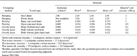
Table 8.3-4 presents factors for estimating percent chemical remaining in drums and tanks after unloading. These factors were derived from a pilot scale research project investigating the effect of the design configuration of the equipment, the method of removing or unloading the chemical from the equipment, the viscosity of the chemical, and the material of construction or lining of the equipment on residue quantities (PEI, 1986). It was concluded that the amount of residue is generally influenced most by the method of unloading. The viscosity of the chemical and the design configuration of the equipment appeared to affect residue quantities to a lesser degree. Material of construction or lining of the equipment appeared to have little effect on residue quantities. The values listed in the table represent residue quantities as a weight percent of vessel capacity (pounds chemical residue per 100 pounds of chemical). The values presented in Table 8.3-4 may be used to represent typical residues, which should only be applied to similar vessel types, unloading methods, and bulk fluid materials. The research was performed with materials with viscosities below 100 cp. For materials with significantly higher viscosities (>200 cp), estimates of percent residue were made based on engineering judgment.
Example 8.3-4
A facility purchased 42,500 pounds of hydrazine this year. To determine the value of the hydrazine lost as residual, the company requests us to provide estimated releases from cleaning the emptied 55-gallon drums.
Solution: You know that the hydrazine is received in steel drums and is pumped into a process vessel. A chemical handbook shows that the viscosities of hydrazine are nearly the same as water at ambient temperatures. Using Table 8.3-4, the loss fraction for water pumped from steel drums is 2.29%. We can use data for water residual as surrogate data for estimating hydrazine residual. Calculation: 42,500 lb/yr 2.29 lb loss/100 lb delivered 973 lb hydrazine estimated to be lost as drum residue.
Table 8.3.4 Summary of Residue Quantities from Pilot-Scale Experimental Study, Weight Percent
8.3.2.6 Secondary Emissions from Utility Sources
Utility consumption in chemical processes is a large generator of environmental impact. Table 8.3-5 lists emission factors for uncontrolled releases for residual and distillate oil combustion. Table 8.3-6 shows similar emission factors for the combustion of natural gas. Each emission factor listed in Tables 8.3-5 and 8.3-6 is based on the volume of fuel burned. In order to relate the emissions of the pollutants to the energy demand in the process, we must first know the fuel value (energy/volume of fuel burned). The efficiency of the boiler supplying the energy transfer agent (steam) needs to be incorporated. The emissions for fuel and natural gas combustion are given by the following general equation:
![]()
where
ED is the energy demand of a process unit (energy demand/unit/yr)
EF is the emission factor for the fuel type (kg/volume of fuel combusted)
FV is the fuel value (energy/volume fuel combusted)
BE is the boiler efficiency (unitless; 0.75 to 0.90 is a typical range of values)
A typical value for the fuel value of natural gas is shown in the footnotes of Table 8.3-6. Typical heating values for solid, liquid, and gaseous fuels are provided in Table 8.3-7. If the boiler efficiency has already been accounted for in the process simulation or analysis, the factor BE is not necessary in the equation above.
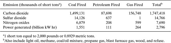
A reasonable approximation for criteria pollutant emission factors (short tons emitted/kW hr) for electricity use in a chemical process can be derived from the data shown in Table 8.3-8 by dividing the emissions by the power generated (bottom row). An average factor (derived from the right column) will be used if the fuel utilized to generate the electricity is not known. The electricity generated by coal, petroleum, and gas fired units does not add to the total electricity generated reported in the table because this total also includes other sources like nuclear power and renewable energy. If not specified in the mass and energy balances for the process, an efficiency for the electric motor or other device must be included. Efficiencies can range from 0.75 to 0.95, depending upon the size and type of the motor. Estimating emissions from electricity consumption in processes is given by;
![]()
where ED is the electricity demand of the unit per year and ME is the efficiency of the device.
Table 8.3-5 Criteria Pollutant Emission Factors (EF) for Uncontrolled Releases from Residual and Distillate Oil Combustion (EPA, 1998).
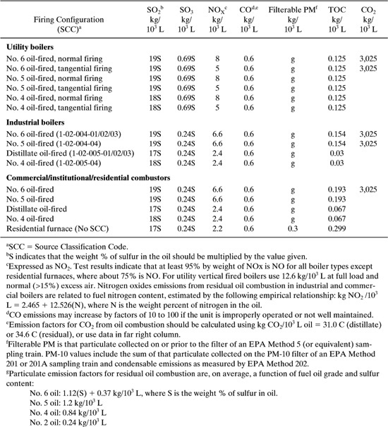
Table 8.3-6 Emission Factors for Sulfur Dioxide (SO2), Nitrogen Oxides (NOx), and Carbon Monoxide (CO) from Natural Gas Combustiona (US EPA, 1998).
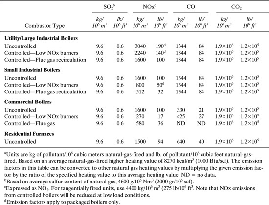
Table 8.3-7 Typical Heating Values for Solid, Liquid, and Gaseous Fuels (Perry and Green, 1997).
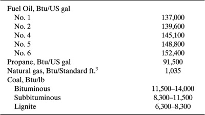
Table 8.3-8 Emissions from Fossil-Fueled Steam-Electric Generating Units (EFacts, 1992).
8.3.3 Modeled Release Estimates
Many process design software programs contain rigorous methods for calculating contents of output streams from process equipment, and some of these output streams are points of release of the process. However, process design software often does not account for all of the releases from a process or is not the most efficient method for generating some release estimates. The material below provides guidance and methods for calculating some of the release points not normally included in process design software and conventional methods.
8.3.3.1 Loading Transport Containers
AP-42 (US EPA, 1985), a US EPA document on emissions issues and estimation methods, discusses the estimation of losses due to vapors generated from bulk loading of petroleum products. Additional information on AP-42 can be found in Appendix F. This model and related information should apply to other non-petroleum organic chemicals that can generate vapors. The following discussion of the model and issues contains many excerpts from AP-42.
Loading losses are a primary source of evaporative emissions from rail tank car, tank truck, and similar bulk loading operations. Loading losses occur as vapors in “empty” cargo tanks are displaced to the atmosphere by the liquid being loaded into the tanks. These vapors are a composite of (1) vapors formed in the empty tank by evaporation of residual product from previous loads (if applicable), (2) vapors transferred to the tank in vapor balance systems (discussed below) as product is being unloaded (if applicable), and (3) vapors generated in the tank as the new product is being loaded. The quantity of evaporative losses from loading operations is, therefore, a function of the following parameters:
• Physical and chemical characteristics of the previous cargo.
• Method of unloading the previous cargo.
• Operations to transport the empty carrier to a loading terminal.
• Method of loading the new cargo.
• Physical and chemical characteristics of the new cargo.
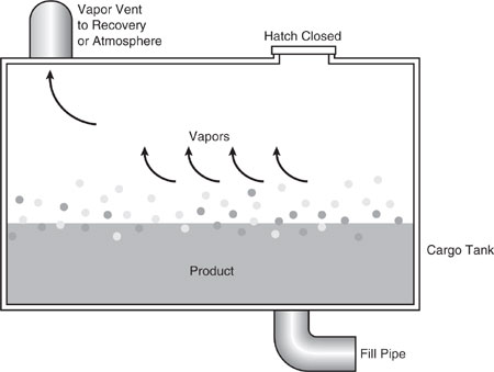
The principal methods of cargo carrier loading are illustrated in Figures 8.3-1, 8.3-2, and 8.3-3. In the splash loading method, the fill pipe dispensing the cargo is lowered only part way into the cargo tank. Significant turbulence and vapor/liquid contact occur during the splash loading operation, resulting in high levels of vapor generation and loss. If the turbulence is great enough, liquid droplets will be entrained in the vented vapors.
A second method of loading is submerged loading. Two types are the submerged fill pipe method and the bottom loading method. In the submerged fill pipe method, the fill pipe extends almost to the bottom of the cargo tank. In the bottom loading method, a permanent fill pipe is attached to the cargo tank bottom. During most of submerged loading by both methods, the fill pipe opening is below the liquid surface level. Liquid turbulence is controlled significantly during submerged loading, resulting in much lower vapor generation than encountered during splash loading. The recent loading history of a cargo carrier is just as important a factor in loading losses as the method of loading. If the carrier has carried a nonvolatile liquid such as fuel oil, or has just been cleaned, it will contain vapor-free air. If it has just carried gasoline and has not been vented, the air in the carrier tank will contain volatile organic vapors, which will be expelled during the loading operation along with newly generated vapors.
Figure 8.3-1 Splash loading method.
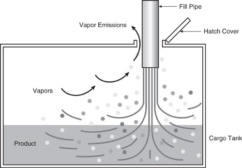
Figure 8.3-2 Submerged fill pipe.
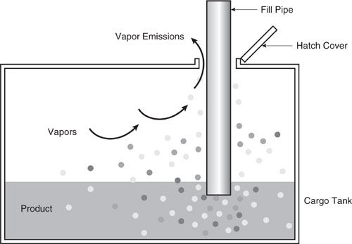
Figure 8.3-3 Bottom loading.
Cargo carriers are sometimes designated to transport only one product, and in such cases are practicing “dedicated service.” Dedicated gasoline cargo tanks return to a loading terminal containing air fully or partially saturated with vapor from the previous load. Cargo tanks may also be “switch loaded” with various products, so that a nonvolatile product being loaded may expel the vapors remaining from a previous load of a volatile product such as gasoline. These circumstances vary with the type of cargo tank and with the ownership of the carrier, the liquids being transported, geographic location, and season of the year.
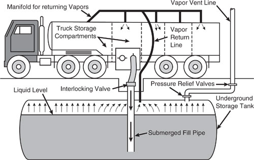
One control measure for vapors displaced during liquid unloading at bulk plants or service stations is called “vapor balance service”. The cargo tank on the truck retrieves the vapors displaced, then the truck transports the vapors back to the loading terminal. Figure 8.3-4 shows a tank truck in “vapor balance service” filling an underground tank and taking on displaced gasoline vapors for return to the terminal. A cargo tank returning to a bulk terminal in “vapor balance service” normally is saturated with organic vapors, and the presence of these vapors at the start of submerged loading of the tanker truck results in greater loading losses than encountered during non-vapor balance, or “normal”, service. Vapor balance service is usually not practiced with marine vessels, although some vessels practice emission control by means of vapor transfer within their own cargo tanks during ballasting operations. More information about ballasting losses may be found in AP-42 section 5.2.2.1.2.
Figure 8.3-4 Tank truck unloading into a service station underground storage tank, practicing “vapor balancing.”
If the evaporation rate is negligible in comparison to the displacement rate, emission losses from loading liquid, given in units of pounds per 1000 gallons of liquid loaded, can be estimated (with a probable error of 30 percent) using Equation 8-7 from AP-42 (US EPA 1985):
![]()
where
LL = loading loss [(lbs/103 gal) of liquid loaded]
S = saturation factor [dimensionless] (see Table 8.3-9)
P = true vapor pressure of liquid loaded [psia]
M = molecular weight of vapors [lb/lb-mole]
T = temperature of bulk liquid loaded [R (F 460)]
This equation can be used for liquids with vapor pressures below 0.68 psia (35 torr). Equation 8-7 can be used to estimate the loading loss of a single chemical in a liquid mixture of two or more chemicals. In such a case, the true vapor pressure of the single chemical may overestimate the loss. If the mole fraction of the chemical in the mixture is expected to be less than unity, we may wish to account for this decrease in the calculated loss. For mixtures, the vapor pressure of a chemical component (Pa in atmospheres) can be calculated using Raoult’s Law as shown in Equation 8-8:
![]()
where
P = Vapor pressure of pure substance, atm
Xa = Mole fraction of component of component a
Raoult’s Law may be too simplistic in certain circumstances. For chemicals that are solid at ambient temperature and volatilize by sublimation, simple techniques for estimating physical properties are not adequate for predicting vapor pressure.
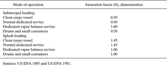
Saturation factors for tank truck loading of petroleum liquids are expected to range from 0.5 to 1.45 (US EPA, 1985). If complete saturation of the vapor space within a vessel is assumed, the saturation factor is equal to 1. Table 8.3-9 lists typical saturation factors by mode of loading for tank trucks, rail cars, drums, and small containers.
In some cases, emission rates, as well as emissions per filling event, must be calculated. The loading loss calculated in Equation 8-7 for vapor being displaced from a container may be converted to a generation rate, which is shown in Equation 8-9. The differences between Equations 8-7 and 8-9 are simply converting units to metric units, separating the universal gas constant R from the equation coefficient, and multiplying by the amount of volume displaced over time (represented by container volume (V) and fill rate (r)).
Table 8.3-9 Saturation Factors for Loading Operations
![]()
where
G = vapor generation of component [g/sec]
S = saturation factor [dimensionless]
M = molecular weight of vapors[g/g-mole]
V = volume of container [cm3]
r = fill rate [containers/hr]
P = vapor pressure of component [atm, at TL]
R = universal gas constant [82.05atm*cm3/g-mol*K]
TL liquid temperature [K]
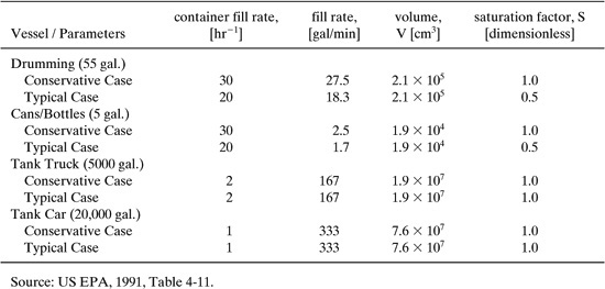
EPA has chosen some default parameters for use when information is not available to determine the actual or expected values of these parameters for a given situation. These default values are shown in Table 8.3-10. Some typical and conservative values for fill rates associated with various transfer operations, with accompanying values for other parameters, are given in Table 8.3-10.
Example 8.3-5
ABC Chemical Company plans to produce and sell 50,000 pounds of n-butyl lactate (NBL) this year. All of this product will be shipped in 55-gallon drums. ABC will produce 5,000 lb/day of NBL for 10 days, and each day’s production is drummed in 30 minutes. How much of the NBL product will be emitted daily as fugitive vapors from ABC’s drumming operation?
Solution: The fugitive emission may be calculated using Equation 8-9, and the parameters needed for the calculation follow (information/data source for each parameter is shown in parentheses).
Table 8.3-10 Transfer Operation Default Parameters for Equation 8-9.
S (saturation factor) = 0.5 (Table 8.3-9, typical chosen)
M (molecular weight of vapor in g/g-mole) = 146.2
V (volume of container in cm3) 2.1 105 (Table 8.3-10 for 55-gal drum) r (fill rate as containers/hr) 5,000 lb/day / [0.98 (specific gravity, NIOSH, 1997) 8.33 lb/gal] / 55 gal/drum 11 drums/day / 0.5 hr/day 22 drums/hr
P (vapor pressure of NBL in atm at TL) 0.4 mm (NIOSH, 1997) / 760 mm/atm 0.0005 atm
R (universal gas constant in atm cm3/g-mol K) 82.05
TL (liquid temperature in K) 68EF 20EC 293 K
These parameters may be placed in the equation:
G =0.5 X146.2 X 210,000 X 22 X 0.0005/13.600 X 82.05 X 2932) = 2.05 X 10⁻³g/sec
= 2.05 X 10⁻³g/sec X 3,600sec/hr X 0.5 hr/day = 3.7 g/day = 3.7 X 10⁻³kg/day
8.3.3.2 Evaporative Losses from Static Liquid Pools
Vapors may be generated from evaporation from pools of liquid that are open to the air. Routine emissions may oocur from open surface operations, which would include work related to open vats or tanks, solvent dip tanks, open roller coating, and cleaning or maintenance activities. More sporadic emissions may occur from liquid pools caused by events such as unintentional spills. A number of models are available to estimate air emissions from open liquid pools, and these models can be used to make very conservative estimates for open tanks used in routine operations. Only one of these models, which is a correltaion developed by US EPA, will be examined to demonstrate a typical approach.
To develop this correlation for EPA, the evaporation rates of 16 different pure compounds in a test chamber were measured to determine an empirical model to describe the relationship between evaporation rate and physical chemical properties. The compounds were studied at different air velocities and temperatures, and the data were curve-fitted. Based on mass balance of a differential element above a liquid pool, the evaporation rate was derived (Hummel, 1996):
![]()
where
G = Generation rate, lb/hr
M = Molecular weight, lb/lb mole
P = Vapor pressure, in. Hg
A = Area, ft2
Dab = Diffusion coefficient, ft2/sec of a through b (in this case b is air)
vz = Air velocity, ft/min
T = Temperature, K
Δz = Pool length along flow direction, ft
Gas diffusivities of volatile compounds in air are available for some chemicals. More often, however, the diffusion coefficient will not be known. An equation to estimate diffusion coefficients (Hummel, et al., 1996, see reference section in Chapter 6) has been developed. The expression for the diffusion coefficient is:
![]()
where
Dab = Diffusion coefficient, cm2/sec
T = Temperature, K
M Molecular weight, g/g-mole
Pt = Pressure, atm
8.3.3.3 Storage Tank Working and Breathing Losses
Storage tanks are units common to almost every chemical process. They provide a buffer for raw materials availability in continuous processes and allow for storage of finished product before delivery is taken. Tanks have the potential to be major contributors to airborne emissions of volatile organic compounds from chemical facilities because of the dynamic operation of these units. There are two major losses mechanisms from tanks; working losses and standing losses. Working losses originate from the raising and lowering of the liquid level in the tank as a result of raw material utilization and production of product. The gas space above the liquid must expand and contract in response to these level changes. During tank emptying, air from the outside or an inert gas will enter the tank. Volatile organic vapors from the liquid will evaporate into the gas in an attempt to achieve an equilibrium condition between the concentrations of each component in the liquid and gas phases. When the tank is filled again, these vapors in the gas will exit the unit via the vent to be dispersed into the atmosphere unless pollution control devices are installed. Even if the tank level is static, standing losses from the tank will occur as a result of daily temperature and ambient pressure fluctuations which cause a pressure difference between the gas inside the tank and the outside air.
There are four major types of storage tanks; fixed-roof, floating-roof, variable-vapor-space, and pressurized tanks. Equations for estimating emissions from fixed-roof and floating-roof storage tanks are provided in Appendix C. Example problems are also included. Software that performs these calculations (the TANKS program) is available from the EPA CHIEF website (http://www.epa.gov/ttn/chief/).
8.3.4 Release Characterization and Documentation
Estimating releases often requires judgment, and the reliability of emission estimates based on judgment is often difficult to assess. The uncertainty depends on how well we know the process, how well we understand the estimation method and its data and parameters, and how well the method and parameters seem to match up with those expected for the actual process. Uncertainties are inherent in making estimations, and the issues of uncertainty are complex. Some uncertainties can be quantified using established methods, but, more frequently, uncertainties cannot be quantified. Often, the factor quality rating system of the US EPA is used in assessing the accuracy and representativeness of emission data. This rating system assigns a quality index of A through E and a U for unratable. Detailed explanations for the ratings of A–D can be found elsewhere (EPA, 1998). A factor rating of A is excellent and is assigned for factors developed from A-rated source tests taken from many randomly chosen facilities in industry. The source category is specific enough to minimize variability within the source population (i.e., one type of reactor or separation device). A factor rating of B is above average and is taken from A-rated source tests from a reasonably large number of facilities, but does not necessarily represent a random sampling of industry. A factor rating of C is average and is the same as a B rating except that the source tests include B-rated source test results. A rating of D is below average and is similar to C except that only a small number of facilities were sampled, there is reason to believe that the factor is not representative of industry, and there appears to be evidence of variability within the source category population. A rating of E is poor because the factor is developed from C- and D-rated test data from a small number of facilities. There is reason to believe that the facilities tested do not represent a random sampling of industry and there is variability within source category population. A rating of U may apply to gross mass balance estimation, deficiencies found with C- and D-rated test data, and use of engineering judgment.
An initial screening of the FIRE database showed that out of the approximately 650 emission factors for process vents and other units, only 10 were rated as A (Shonnard, et al., 1995). These factors were all for secondary emission of trichloroethylene from wastewater treatment plants. There were a total of 22 B-rated emission factors, and except for 3, all were from secondary emissions from wastewater treatment plants. A much broader range of processes and process units was related to the 17 C-rated factors found in FIRE. There were only 43 D-rated factors, and these also covered a range of processes and units. The vast majority of emission factors were rated U, unratable. Clearly, many of the emission estimation procedures developed in this chapter provide only order of magnitude estimates of actual or expected process emissions.
After making release estimates, it can be valuable to look at the estimates and ask whether the estimates seem realistic relative to the process flow streams and relative to one another. The assumptions used to make estimates can be evaluated and the sensitivity of the estimates to selected variables can be assessed.
Case Study
The emission estimation procedures described in this section represent only a small fraction of the emission estimation procedures relevant to chemical processes. Nevertheless, they are representative of the types of emission estimation tools used in chemical process designs. To conclude this section, the collection of emission estimation tools will be applied to the chemical process flowsheet shown in Figure 8.3-5.
This is a process in which cyclohexane is oxidized, producing cyclohexanone and cyclohexanol (a ketone/alcohol mixture). This mixture is used in the manufacture of adipic acid, which in turn is used in the production of nylon.
The first step in estimating the emissions for this flowsheet, as outlined in this section, is to identify major emission sources. Among the major sources of emissions from this process are:
• venting from the feed and product storage tanks
• off-gases from the scrubbers
• liquid wastes from the scrubbers
• emissions from the decanting and purification columns
• emissions from the boilers
• fugitive emissions
• feed and product loading and off-loading emissions
Each of these emissions can be calculated, at varying levels of detail, using the methods described in this chapter.
Consider first the emissions from reactors and the emissions from the stripper and the decanting and purification columns. Since no direct process data have been provided for these units, the emissions should be estimated from the general emission factors listed in Table 8.3-2. The relevant factors are 1.5 kg/103 kg throughput for reactor vents, 0.2 kg/103 kg throughput for the stripper, 0.02 kg/103 kg throughput for decanters, and 0.7 kg/103 kg throughput for distillation column vents. For the reactor, we might assume that half of the emissions are reactants (cyclohexane), and half are products (ketone and aldehyde). For the stripper, decanter, and distillation columns, it can be assumed that all of the emissions are product.
Figure 8.3-5 Chemical process flowsheet for case study.
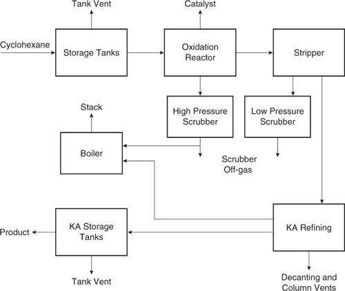
This leads to total emissions for this section of 0.8 kg/103 kg throughput for cyclohexane and 1.6 kg/103 kg throughput for the ketone and alcohol.
A next step in the emission estimation process would be to consider emissions from boilers. To estimate these emissions, an estimate of energy consumption per kg product is required. Rudd, et al. (1981) provide estimates of energy consumption for a number of processes and suggest a value of 0.5 metric tons of fuel oil equivalent per metric ton (103 kg) of product. Assuming that #6 fuel oil with 1% sulfur is used and that no emission controls are in place leads to estimates (based on Table 8.3-5) of:
SO2 emissions:
19kg/103L fuel oil X 0.8kg/L X 500kg fuel oil/103kg product = 7.6kg SO2/103kg product
SO3 emissions:
0.69kg/103L fuel oil X 0.8kg/L X 500kg fuel oil/103kg product = 0.3 SO3/103kg product
8 kg/103 L fuel oil X 0.8 kg/L X 500 kg fuel oil/103kg product 3.2 kg NOx/103 kg product
Particulate Matter emissions:
1.5kg/103 L fuel oil X 0.8kg/L X 500 kg fuel oil/103kg product =0.6kg PM/103 kg prodcut
Accurately estimating fugitive emissions requires a count of valves, flanges, fittings, pumps, and other devices that are used in the process. Such counts are not generally available for preliminary process designs; however, rough estimates can be made based on experience. Typically, fugitive emissions for chemical processes total 0.5–1.5 kg per 103 kg product (Berglund and Hansen, 1990). In this case, we have probably already accounted for some of the fugitive emissions through the emission factors for the reactors and distillation column; therefore, an estimate of 0.5 kg per 103 kg product is appropriate, with the emissions evenly split between products and reactants.
The remaining emissions include emissions from tanks, emissions from loading and off-loading emissions and the off-gases and liquid wastes from the scrubbers. The loading and off-loading emissions could be estimated using Equation 8-7. Assuming a saturation factor of 0.6 (Table 8.3-9), a vapor pressure of 4.1 mm Hg for the ketone (estimated using the methods described in Chapter 5), a molecular weight of 98, and a temperature of 530 R gives a loading loss of:
LL = 12.46(0.6x4.1x(14.7/760)x98/530) = 0.1 lb/103 gal = 0.15kg/103kg product
Losses from tanks can be estimated using the methods described in Appendix C. Without a detailed flowsheet, exact specifications for the tank are not available. A rough estimate of tank dimensions, however, can be derived from annual production rates. If we assume a production rate of 100 million pounds per year, and that a typical tank should hold 2–3 days of production capacity, an approximate tank volume can be calculated. For this production rate, a tank 35 ft in diameter and 20 feet high with a fixed roof, is reasonable. We will also assume that, to minimize emissions, the tank is painted white, the paint is in good condition and the tank is generally kept 80% full. If the facility is located in Houston, Texas, the data and procedures described in the appendix lead to an estimate of order 0.5 kg emitted /103 kg product for standing and working losses. We will assume that these are emissions of the feed material, cyclohexane.
Finally, emission rates should be estimated for the off-gases and liquid wastes from the scrubbers. These emissions depend strongly on the assumed efficiency of the scrubbers. If data are not available for the process of interest, it is generally a sound practice to obtain data from similar processes. For this part of the adipic acid process, AP-42 reports the gas emissions from the scrubbers shown in Table 8.3-11.
Hedley, et al., report rates of liquid waste generation from the combined scrubbers. They suggest approximately 200 kg of organic sodium salts are generated in the scrubbers per 103 kg product.
Table 8.3-11 Gas Phase Emissions from the Scrubbers in Cyclohexane Partial Oxidation (AP-42).
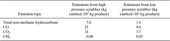
The data summarized in Table 8.3-12 provide a reasonable starting point for estimating the environmental impacts of this chemical process. The next section describes how these emission and other data can be converted to a set of environmental performance metrics.
Table 8.3-12 Preliminary Emission Estimates for the Cyclohexane Partial Oxidation Process (kg emitted /103 kg product).
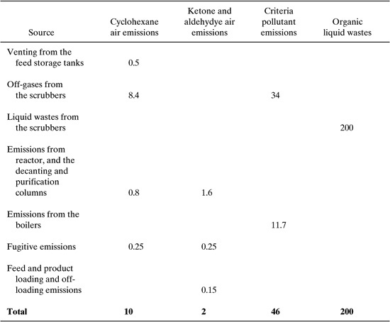
8.3.5 Assessing Environmental Performance
Once preliminary estimates of material flows, energy requirements, wastes and emissions have been made for a flowsheet, the overall environmental performance of the flowsheet can be evaluated. Two types of assessments have been commonly employed. One type of assessment evaluates the treatability or costs of treatment of the waste streams. Douglas and co-workers (Schultz, 1998) have suggested approximate costs for the treatment of waste streams. A second method for assessing environmental performance of flowsheets is to evaluate a set of relatively simple environmental performance indicators. The performance indicators that will be used in this chapter were developed by the Canadian National Roundtable on the Environment and the Economy (NRTEE, 1999). These indicators have been tested and evaluated by a number of organizations throughout North America (including the American Institute of Chemical Engineer’s Center for Waste Reduction Technologies; see CWRT, 1998, 1999). The indicators are:
• Energy consumed from all sources within the manufacturing or delivery process per unit of manufactured output (with electricity consumption converted to equivalent fuel use, based on an average efficiency of converting energy to electricity in power plants).
• Total mass of materials used directly in the product, minus the mass of the product, per unit of manufactured output.
• Water consumption (including water present in waste streams, contact cool-ing water, water vented to the atmosphere, and the fraction of non-contact cooling water lost to evaporation) per unit of manufactured output.
• Emissions of targeted pollutants (those listed in the Toxic Release Inventory) per unit of manufactured output.
• Total pollutants (including acidifying emissions, eutrophying emissions, salinity, and ozone depleting substances) per unit of manufactured output.
Taken together, these cost and environmental performance metrics provide additional guidance on the performance of flowsheets. Consider how the these performance evaluations would be applied to the cyclohexane oxidation process described in the previous section.
Material use for this process can be determined based on the data of Rudd, et al. (1981) and Hedley, et al. (1975). Rudd reports that the manufacture of 1 ton of cyclohexanol requires 1.64 tons of cyclohexane and 0.13 ton of sodium hydroxide. Cyclohexanone is produced at a rate of 0.38 tons per ton of cyclohexanol. If we assume that both cyclohexanone and cyclohexanol are desirable products, then the material intensity (excluding water) is:
Material intensity = [(1.64 + 0.13) tons raw materials - 1.38 pounds product]/(1 + 0.38) tons product = 0.28
Water use has been estimated by Hedley, et al. as 5,000 gpm of cooling water and 10 gpm of process water (used in the scrubber) for a 85,000,000 pound per year facility. This leads to an estimate of approximately 30 gallons of water per pound of product, with most of this water use dedicated to cooling.
Energy intensity is approximately 0.4 L fuel oil per kg product; assuming 150,000 BTU per gallon for fuel oil, this leads to an energy intensity of 7 kBTU per pound of product.
Pollutant generation, which is dominated by organic liquid wastes, is estimated to be approximately 0.3 lb/lb product (Table 8.3-12).
What do these indices mean? Are the values high? Are they low? The best way to evaluate the indices is to consider how other chemical manufacturing processes fare. Table 8.3-13 is a listing of environmental performance indices for a number of chemical manufacturing processes. These were derived by E. Beaver and colleagues in an analysis of chemical manufacturing processes conducted for the Department of Energy (Bridges to Sustainability, 2000).
The sample results shown in Table 8.3-13 reveal that different processes can have dramatically different characteristics. For example, water use, material use, and energy use per pound of product are significantly different for acetic acid, acrylonitrile, and maelic anhydride. This implies that the metrics are sensitive to process designs and chemistry. Data for two different routes for producing sulfuric acid, also shown in Table 8.3-13, reveal that the metrics are sensitive to process design.
With this as background, the metrics obtained for the cyclohexane oxidation can be put in context. Recall that the preliminary estimates for the cyclohexane oxidation flowsheet were:
Material use: | 0.28 lb/lb prod. |
Energy use: | 7 kBTU/lb prod. |
Water use: | 30 gal/lb prod. |
Pollutants: | 0.3 lb/lb prod. |
Table 8.3-13 Representative Environmental Performance Metrics for Chemical Manufacturing Processes (Bridges to Sustainability, 2000).
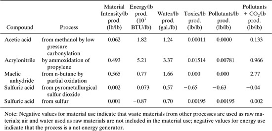
These values are at the high end of the range reported in Table 8.3-13, suggesting that a number of process improvements may be possible. Chapter 9 will describe approaches to identifying process improvements.
Section 8.3 Questions for Discussion
1. What are the major sources of emissions from chemical manufacturing processes?
2. Describe the sources of uncertainty in estimating emissionsfrom process flowsheets.
3. Describe how you might use the benchmark data on environmental metrics for chemical processes. Specifically, consider what types of processes can be compared. Does it make sense to compare the data from a partial oxidation reaction to the data from a cracking reaction?
8.4 Tier 3 Environmental Performance Tools
Once the basic structure of the process flowsheet is determined, detailed specifications of reactor and separator sizes, stream compositions, energy loads, and other process variables can be established. This level of process specification is, once again, an appropriate time to examine environmental performance. At this stage of analysis, a relatively limited number of design alternatives will be screened, but more information about the process is available and should be incorporated into each environmental performance evaluation. Chapter 11 examines methods for evaluating environmental performance at this final level. Before those methods are presented, Chapters 9 and 10 examine methods for improving (as opposed to assessing) environmental performance at the level of a conceptual process flowsheet.
References
Allen, D.T. and Rosselot, K.S., Pollution Prevention for Chemical Processes, John Wiley & Sons, New York, NY, 434 pages, 1997.
American Institute of Chemical Engineers, Center for Waste Reduction Technologies(CWRT), “Sustainability Metrics Interim Report #1,” AIChE CWRT, New York, 1998.
American Institute of Chemical Engineers, Center for Waste Reduction Technologies(CWRT), “Sustainability Metrics Interim Report #2,” AIChE CWRT, New York, 1999.
Berglund, R. L., Wood, D.A. and Covin, T. J. “Fugitive emissions from the acrolein production industry,” in the Air and Waste Management Association International Specialty Conference: SARA Title III, Section 313, Industry Experience in Estimating Chemical Releases, April 6, 1989.
Bridges to Sustainability, “Sustainability Metrics: Making Decisions for Major Chemical
Products and Facilities,” Houston, Texas (2000).
Chang, D., M.S. Thesis, University of California, Los Angeles, 1996.
Crowl, D. A., and Louvar, J.F., Chemical Process Safety: Fundamentals with Applications, Prentice Hall, Englewood Cliffs, New Jersey, 1990.
Douglas, J.M., Conceptual Design of Chemical Processes, McGraw Hill, New York, 1988.
Energy Facts 1992, Energy Information Administration, U.S. Department of Energy, DOE/EIA-0469 (1992).
Hedley, W.H., Mehta, S.M., Moscowitz, C.M., Reznik, R.B., Richardson, G.A., and Zanders, D.L., Potential Pollutants from Petrochemical Processes, Technomic, Westport, Conn., 1975.
National Roundtable on the Environment and the Economy (NRTEE), Measuring Eco-efficiency in Business: Feasibility of a Core Set of Indicators, Renouf Publishing, Ottowa Canada, 1999 (ISBN 1-895643-98-8).
PEI, 1986, “Releases during Cleaning of Equipment,” Report prepared under Contract 68-02-4248 to US EPA, Office of Toxic Substances.
Perry, R. H. and Green, D. W., Perry’s Chemical Engineers’ Handbook, 7th Edition, McGraw-Hill Book Company, New York, NY, 1997.
Rudd, D.F., Fathi-Afshar, S., Trevino, A., and Stahtherr, M.A., Petrochemical Technology Assessment, Wiley-Interscience, New York, 1981.
Schultz, M. A., “A Hierarchical Design Procedure for the Conceptual Design of Pollution Prevention Alternatives for Chemical Processes,” Ph.D. Thesis, University of Massachusetts, 1998.
Shonnard, D. R., Markey, J. M., and Deshpande, P. A., “Evaluation of unit operations and ic emission databases,” the Proceedings of the 1995 American Institute of Chemical Engineers Summer National Meeting, Boston, Mass., August, 1995.
US EPA, “Organic Chemical Manufacturing: Selected Processes,” US Environmental Protection Agency, Research Triangle Park, NC, 1980, EPA-450/3-80-028c.
US EPA, “Compilation of Air Pollutant Emission Factors, Volume I: Stationary Point and Area Sources,” 4th edition, with Supplements A-D, US Environmental Protection Agency, Research Triangle Park, NC, Publication AP-42, 1985.
US EPA, “Estimating Releases and Waste Treatment Efficiencies for the Toxic Chemical
Release Inventory Form” (EPA/560/4-88-002), US Environmental Protection Agency, Washington, D.C. (1987).
US EPA, “Toxic Air Pollutant Emission Factors - A Compilation of Selected Air Toxic Compounds and Sources” (EPA/450/2-88-006a), US Environmental Protection Agency, Washington, D.C. (1988).
US EPA, “Locating and Estimating Air Emissions,” US Environmental Protection Agency, Research Triangle Park, NC, Report Number EPA-450/4-, 1979-1991.
US EPA, “Protocol for Equipment Leak Emission Estimates,” US Environmental Protection Agency, Research Triangle Park, NC, available through NTIS (PB93-229219, June, 1993.
US EPA, Integrated Risk Information System (IRIS), http://www.epa.gov/ngispgm3/iris/Substance_List.html, US Environmental Protection Agency, 1997.
US EPA, “Compilation Of Air Pollutant Emission Factors, Volume I, Fifth Edition,” AP-42, Air CHIEF CD-ROM, ClearingHouse For Inventories And Emission Factors, Air CHIEF CD-ROM, (EFIG/EMAD/OAQPS/EPA), Version 6.0, U.S. Environmental Protection Agency, Research Triangle Park, NC, EPA-454/F-98-007, 1998 (see also http://www.epa.gov/ttn/chief/).
Wagner, P.M., Nabholz, J.V., and Kent, R.J., “The new chemicals process at the Environmental Protection Agency (EPA): structure activity relationships for hazard identification and risk assessment,” Toxicology Letters, 79, 67-73 (1995).
Problems
1. Compare the carbonylation of dinitrotoluene and the amine-phosgene routes for the production of toluene diisocyanate (TDI) using a Tier 1 economic and environmental performance evaluation. The amine-phosgene route involves the reaction of phosgene with toluenediamine in a chlorobenzene solvent. The carbonylation route has been demonstrated in laboratories, but is not presently a commercial technology. Data from the patent literature (see the Green Chemistry Expert System, Appendix F) indicate that the reaction of 2,4 dinitrotoluene with carbon monoxide occurs over a mixed oxide catalyst. Conversion approaches 100% with selectivity to the desired product ranging from 70–99%. Laboratory data indicate that the reaction can be performed in a chlorobenzene and pyridine solvent. Approximate stoichiometric data, based on the patent data, are given in the table below.
Amine-phosgene route:
C6H3(CH3)(NH2)2+ 2COCI2 → C6H3(CH3)(→N = C = O)2 + 4 HCI
Carbonylation of dinitrotoluene:
C6H3(CH3)(NO2)2 + 6CO → C6H3(CH3)(– N =C=O)2 + 4CO2
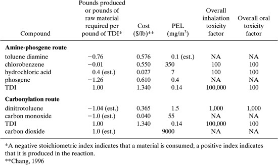
(a) Identify major sources of emissions.
(b) Using the methods described in this chapter and data available in AP-42 documents available on-line (http://www.epa.gov/ttn/chief/), estimate wastes and emissions for this process.