After studying this chapter, you should be able to:
The Magic Of Interest
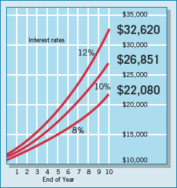
Sidney Homer, author of A History of Interest Rates, wrote, "$1,000 invested at a mere 8 percent for 400 years would grow to $23 quadrillion—$5 million for every human on earth. But the first 100 years are the hardest." This startling quote highlights the power of time and compounding interest on money. Equally significant, although Homer did not mention it, is the fact that a small difference in the interest rate makes a big difference in the amount of monies accumulated over time.
Taking an example more realistic than Homer's 400-year investment, assume that you had $20,000 in a tax-free retirement account. Half the money is in stocks returning 12 percent, and the other half is in bonds earning 8 percent. Assuming reinvested profits and quarterly compounding, your bonds would be worth $22,080 after 10 years, a doubling of their value. But your stocks, returning 4 percent more, would be worth $32,620, or triple your initial value. The following chart shows this impact.
Because of interest paid on investments, money received a week from today is not the same as money received today. Business people are acutely aware of this timing factor, and they invest and borrow only after carefully analyzing the relative amounts of cash flows over time.
With the profession's movement toward fair value accounting and reporting, an understanding of present value calculations is imperative. As an example, companies now have the option to report most financial instruments (both assets and liabilities) at fair value. In many cases, a present value computation is needed to arrive at the fair value amount, particularly as it relates to liabilities. In addition, the recent controversy involving the proper impairment charges for mortgage-backed receivables highlights the necessity to use present value methodologies when markets for financial instruments become unstable or nonexistent.
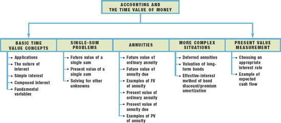
PREVIEW OF CHAPTER 6
As we indicated in the opening story, the timing of the returns on an investment has an important effect on the worth of the investment (asset). Similarly, the timing of debt repayment has an important effect on the value of the debt commitment (liability). As a financial expert, you will be expected to make present and future value measurements and to understand their implications. The purpose of this chapter is to present the tools and techniques that will help you measure the present value of future cash inflows and outflows. The content and organization of the chapter are as follows.
In accounting (and finance), the phrase time value of money indicates a relationship between time and money—that a dollar received today is worth more than a dollar promised at some time in the future. Why? Because of the opportunity to invest today's dollar and receive interest on the investment. Yet, when deciding among investment or borrowing alternatives, it is essential to be able to compare today's dollar and tomorrow's dollar on the same footing—to "compare apples to apples." Investors do that by using the concept of present value, which has many applications in accounting.
Financial reporting uses different measurements in different situations—historical cost for equipment, net realizable value for inventories, fair value for investments. As we discussed in Chapter 2, the FASB increasingly is requiring the use of fair values in the measurement of assets and liabilities. According to the FASB's recent guidance on fair value measurements, the most useful fair value measures are based on market prices in active markets. Within the fair value hierarchy these are referred to as Level 1. Recall that Level 1 fair value measures are the most reliable because they are based on quoted prices, such as a closing stock price in the Wall Street Journal.
However, for many assets and liabilities, market-based fair value information is not readily available. In these cases, fair value can be estimated based on the expected future cash flows related to the asset or liability. Such fair value estimates are generally considered Level 3 (least reliable) in the fair value hierarchy because they are based on unobservable inputs, such as a company's own data or assumptions related to the expected future cash flows associated with the asset or liability. As discussed in the fair value guidance, present value techniques are used to convert expected cash flows into present values, which represent an estimate of fair value. [1]
Because of the increased use of present values in this and other contexts, it is important to understand present value techniques.[73] We list some of the applications of present value-based measurements to accounting topics below; we discuss many of these in the following chapters.
In addition to accounting and business applications, compound interest, annuity, and present value concepts apply to personal finance and investment decisions. In purchasing a home or car, planning for retirement, and evaluating alternative investments, you will need to understand time value of money concepts.
Interest is payment for the use of money. It is the excess cash received or repaid over and above the amount lent or borrowed (principal). For example, Corner Bank lends Hillfarm Company $10,000 with the understanding that it will repay $11,500. The excess over $10,000, or $1,500, represents interest expense.
The lender generally states the amount of interest as a rate over a specific period of time. For example, if Hillfarm borrowed $10,000 for one year before repaying $11,500, the rate of interest is 15 percent per year ($1,500 ÷ $10,000). The custom of expressing interest as a percentage rate is an established business practice.[74] In fact, business managers make investing and borrowing decisions on the basis of the rate of interest involved, rather than on the actual dollar amount of interest to be received or paid.
How is the interest rate determined? One important factor is the level of credit risk (risk of nonpayment) involved. Other factors being equal, the higher the credit risk, the higher the interest rate. Low-risk borrowers like Microsoft or Intel can probably obtain a loan at or slightly below the going market rate of interest. However, a bank would probably charge the neighborhood delicatessen several percentage points above the market rate, if granting the loan at all.
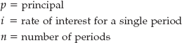
The amount of interest involved in any financing transaction is a function of three variables:
Thus, the following three relationships apply:
The larger the principal amount, the larger the dollar amount of interest.
The higher the interest rate, the larger the dollar amount of interest.
The longer the time period, the larger the dollar amount of interest.
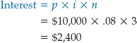
Companies compute simple interest on the amount of the principal only. It is the return on (or growth of) the principal for one time period. The following equation expresses simple interest.[75]
where
To illustrate, Barstow Electric Inc. borrows $10,000 for 3 years with a simple interest rate of 8% per year. It computes the total interest it will pay as follows.
If Barstow borrows $10,000 for 3 months at 8%, the interest is $200, computed as follows.
John Maynard Keynes, the legendary English economist, supposedly called it magic. Mayer Rothschild, the founder of the famous European banking firm, proclaimed it the eighth wonder of the world. Today, people continue to extol its wonder and its power. The object of their affection? Compound interest.
We compute compound interest on principal and on any interest earned that has not been paid or withdrawn. It is the return on (or growth of) the principal for two or more time periods. Compounding computes interest not only on the principal but also on the interest earned to date on that principal, assuming the interest is left on deposit.
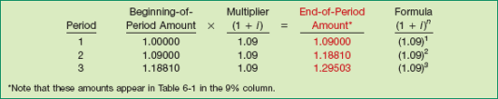
To illustrate the difference between simple and compound interest, assume that Vasquez Company deposits $10,000 in the Last National Bank, where it will earn simple interest of 9% per year. It deposits another $10,000 in the First State Bank, where it will earn compound interest of 9% per year compounded annually. In both cases, Vasquez will not withdraw any interest until 3 years from the date of deposit. Illustration 6-1 shows the computation of interest Vasquez will receive, as well as its accumulated year-end balance.
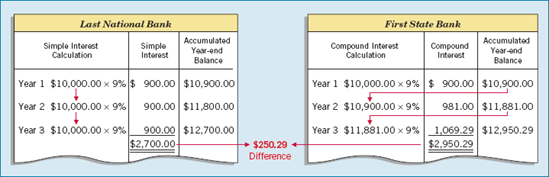
Note in Illustration 6.1 that simple interest uses the initial principal of $10,000 to compute the interest in all 3 years. Compound interest uses the accumulated balance (principal plus interest to date) at each year-end to compute interest in the succeeding year. This explains the larger balance in the compound interest account.
Obviously, any rational investor would choose compound interest, if available, over simple interest. In the example above, compounding provides $250.29 of additional interest revenue. For practical purposes, compounding assumes that unpaid interest earned becomes a part of the principal. Furthermore, the accumulated balance at the end of each year becomes the new principal sum on which interest is earned during the next year.
Compound interest is the typical interest computation applied in business situations. This occurs particularly in our economy, where companies use and finance large amounts of long-lived assets over long periods of time. Financial managers view and evaluate their investment opportunities in terms of a series of periodic returns, each of which they can reinvest to yield additional returns. Simple interest usually applies only to short-term investments and debts that involve a time span of one year or less.
The continuing debate on Social Security reform provides a great context to illustrate the power of compounding. One proposed idea is for the government to give $1,000 to every citizen at birth. This gift would be deposited in an account that would earn interest tax-free until the citizen retires. Assuming the account earns a modest 5% annual return until retirement at age 65, the $1,000 would grow to $23,839. With monthly compounding, the $1,000 deposited at birth would grow to $25,617.
Why start so early? If the government waited until age 18 to deposit the money, it would grow to only $9,906 with annual compounding. That is, reducing the time invested by a third results in more than a 50% reduction in retirement money. This example illustrates the importance of starting early when the power of compounding is involved.
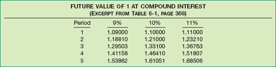
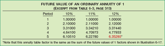
We present five different types of compound interest tables at the end of this chapter. These tables should help you study this chapter as well as solve other problems involving interest.
Illustration 6-2 lists the general format and content of these tables. It shows how much principal plus interest a dollar accumulates to at the end of each of five periods, at three different rates of compound interest.
The compound tables rely on basic formulas. For example, the formula to determine the future value factor (FVF) for 1 is:
where
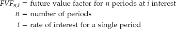

Financial calculators include preprogrammed FVFn,i and other time value of money formulas.
To illustrate the use of interest tables to calculate compound amounts, assume an interest rate of 9%. Illustration 6-3 shows the future value to which 1 accumulates (the future value factor).
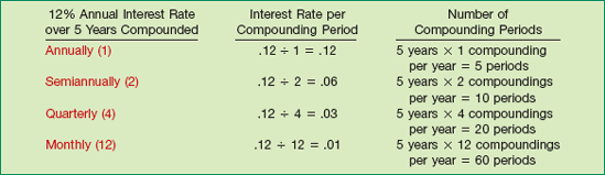
Throughout our discussion of compound interest tables, note the intentional use of the term periods instead of years. Interest is generally expressed in terms of an annual rate. However, many business circumstances dictate a compounding period of less than one year. In such circumstances, a company must convert the annual interest rate to correspond to the length of the period. To convert the "annual interest rate" into the "compounding period interest rate," a company divides the annual rate by the number of compounding periods per year.
In addition, companies determine the number of periods by multiplying the number of years involved by the number of compounding periods per year. To illustrate, assume an investment of $1 for 6 years at 8% annual interest compounded quarterly. Using Table 6-1, page 308, read the factor that appears in the 2% column on the 24th row—6 years × 4 compounding periods per year, namely 1.60844, or approximately $1.61. Thus, all compound interest tables use the term periods, not years, to express the quantity of n. Illustration 6-4 shows how to determine (1) the interest rate per compounding period and (2) the number of compounding periods in four situations of differing compounding frequency.[76]
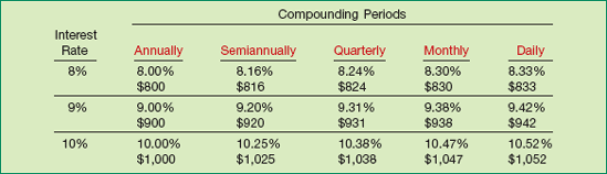
How often interest is compounded can substantially affect the rate of return. For example, a 9% annual interest compounded daily provides a 9.42% yield, or a difference of 0.42%. The 9.42% is the effective yield.[77] The annual interest rate (9%) is the stated, nominal, or face rate. When the compounding frequency is greater than once a year, the effective interest rate will always exceed the stated rate.
Illustration 6-5 shows how compounding for five different time periods affects the effective yield and the amount earned by an investment of $10,000 for one year.
The following four variables are fundamental to all compound interest problems.
Illustration 6-6 depicts the relationship of these four fundamental variables in a time diagram.
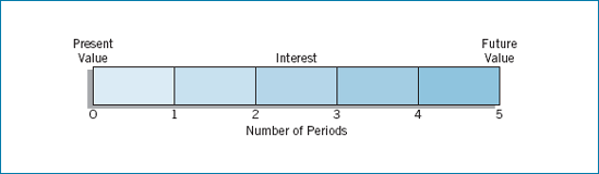
In some cases, all four of these variables are known. However, at least one variable is unknown in many business situations. To better understand and solve the problems in this chapter, we encourage you to sketch compound interest problems in the form of the preceding time diagram.
Many business and investment decisions involve a single amount of money that either exists now or will in the future. Single-sum problems are generally classified into one of the following two categories.
Computing the unknown future value of a known single sum of money that is invested now for a certain number of periods at a certain interest rate.
Computing the unknown present value of a known single sum of money in the future that is discounted for a certain number of periods at a certain interest rate.
When analyzing the information provided, determine first whether the problem involves a future value or a present value. Then apply the following general rules, depending on the situation:
If solving for a future value, accumulate all cash flows to a future point. In this instance, interest increases the amounts or values over time so that the future value exceeds the present value.
If solving for a present value, discount all cash flows from the future to the present. In this case, discounting reduces the amounts or values, so that the present value is less than the future amount.
Preparation of time diagrams aids in identifying the unknown as an item in the future or the present. Sometimes the problem involves neither a future value nor a present value. Instead, the unknown is the interest or discount rate, or the number of compounding or discounting periods.
To determine the future value of a single sum, multiply the future value factor by its present value (principal), as follows.
where
To illustrate, Bruegger Co. wants to determine the future value of $50,000 invested for 5 years compounded annually at an interest rate of 11%. Illustration 6-7 shows this investment situation in time-diagram form.
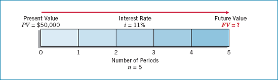
Using the future value formula, Bruegger solves this investment problem as follows.
To determine the future value factor of 1.68506 in the formula above, Bruegger uses a financial calculator or reads the appropriate table, in this case Table 6-1 (11% column and the 5-period row).
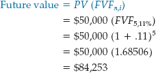
Companies can apply this time diagram and formula approach to routine business situations. To illustrate, assume that Commonwealth Edison Company deposited $250 million in an escrow account with Northern Trust Company at the beginning of 2010 as a commitment toward a power plant to be completed December 31, 2013. How much will the company have on deposit at the end of 4 years if interest is 10%, compounded semiannually?
With a known present value of $250 million, a total of 8 compounding periods (4 × 2), and an interest rate of 5% per compounding period (.10 ÷ 2), the company can time-diagram this problem and determine the future value as shown in Illustration 6-8.
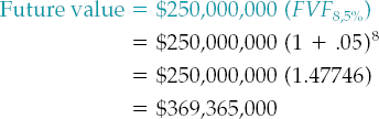
Using a future value factor found in Table 1 (5% column, 8-period row), we find that the deposit of $250 million will accumulate to $369,365,000 by December 31, 2013.
The Bruegger example on page 271 showed that $50,000 invested at an annually compounded interest rate of 11% will equal $84,253 at the end of 5 years. It follows, then, that $84,253, 5 years in the future, is worth $50,000 now. That is, $50,000 is the present value of $84,253. The present value is the amount needed to invest now, to produce a known future value.
The present value is always a smaller amount than the known future value, due to earned and accumulated interest. In determining the future value, a company moves forward in time using a process of accumulation. In determining present value, it moves backward in time using a process of discounting.
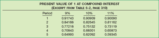
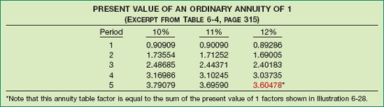
As indicated earlier, a "present value of 1 table" appears at the end of this chapter as Table 6-2. Illustration 6-9 demonstrates the nature of such a table. It shows the present value of 1 for five different periods at three different rates of interest.
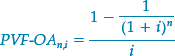
The following formula is used to determine the present value of 1 (present value factor):
where
PVFn,i = present value factor for n periods at i interest
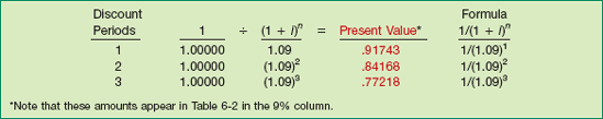
To illustrate, assuming an interest rate of 9%, the present value of 1 discounted for three different periods is as shown in Illustration 6-10.
The present value of any single sum (future value), then, is as follows.
where
| PV = present value |
| FV = future value |
| PVFn,i = present value factor for n periods at i interest |
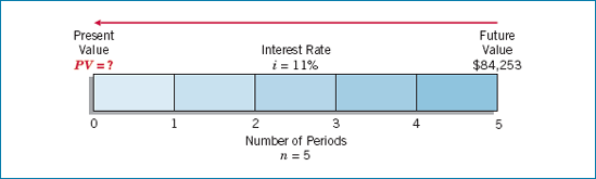
To illustrate, what is the present value of $84,253 to be received or paid in 5 years discounted at 11% compounded annually? Illustration 6-11 shows this problem as a time diagram.
Using the formula, we solve this problem as follows.
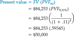
To determine the present value factor of 0.59345, use a financial calculator or read the present value of a single sum in Table 6-2 (11% column, 5-period row).
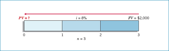
The time diagram and formula approach can be applied in a variety of situations. For example, assume that your rich uncle decides to give you $2,000 for a trip to Europe when you graduate from college 3 years from now. He proposes to finance the trip by investing a sum of money now at 8% compound interest that will provide you with $2,000 upon your graduation. The only conditions are that you graduate and that you tell him how much to invest now.
To impress your uncle, you set up the time diagram in Illustration 6-12 and solve this problem as follows.
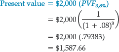
Advise your uncle to invest $1,587.66 now to provide you with $2,000 upon graduation. To satisfy your uncle's other condition, you must pass this course (and many more).
In computing either the future value or the present value in the previous single-sum illustrations, both the number of periods and the interest rate were known. In many business situations, both the future value and the present value are known, but the number of periods or the interest rate is unknown. The following two examples are single-sum problems (future value and present value) with either an unknown number of periods (n) or an unknown interest rate (i). These examples, and the accompanying solutions, demonstrate that knowing any three of the four values (future value, FV; present value, PV; number of periods, n; interest rate, i) allows you to derive the remaining unknown variable.
The Village of Somonauk wants to accumulate $70,000 for the construction of a veterans monument in the town square. At the beginning of the current year, the Village deposited $47,811 in a memorial fund that earns 10% interest compounded annually. How many years will it take to accumulate $70,000 in the memorial fund?
In this illustration, the Village knows both the present value ($47,811) and the future value ($70,000), along with the interest rate of 10%. Illustration 6-13 depicts this investment problem as a time diagram.
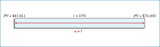
Knowing both the present value and the future value allows the Village to solve for the unknown number of periods. It may use either the future value or the present value formulas, as shown in Illustration 6-14.
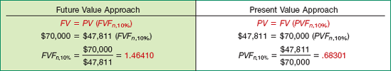
Using the future value factor of 1.46410, refer to Table 6-1 and read down the 10% column to find that factor in the 4-period row. Thus, it will take 4 years for the $47,811 to accumulate to $70,000 if invested at 10% interest compounded annually. Or, using the present value factor of 0.68301, refer to Table 6-2 and read down the 10% column to find that factor in the 4-period row.
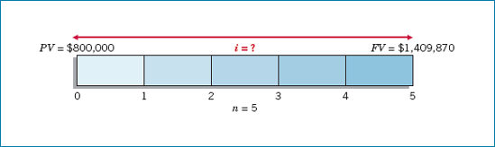
Advanced Design, Inc. needs $1,409,870 for basic research 5 years from now. The company currently has $800,000 to invest for that purpose. At what rate of interest must it invest the $800,000 to fund basic research projects of $1,409,870, 5 years from now?
The time diagram in Illustration 6-15 depicts this investment situation.
Advanced Design may determine the unknown interest rate from either the future value approach or the present value approach, as Illustration 6-16 shows.
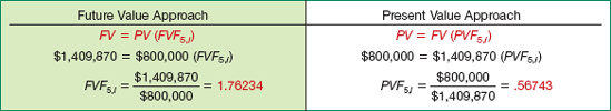
Using the future value factor of 1.76234, refer to Table 6-1 and read across the 5-period row to find that factor in the 12% column. Thus, the company must invest the $800,000 at 12% to accumulate to $1,409,870 in 5 years. Or, using the present value factor of .56743 and Table 6-2, again find that factor at the juncture of the 5-period row and the 12% column.
The preceding discussion involved only the accumulation or discounting of a single principal sum. However, many situations arise in which a series of dollar amounts are paid or received periodically, such as installment loans or sales; regular, partially recovered invested funds; or a series of realized cost savings.
For example, a life insurance contract involves a series of equal payments made at equal intervals of time. Such a process of periodic payment represents the accumulation of a sum of money through an annuity. An annuity, by definition, requires the following: (1) periodic payments or receipts (called rents) of the same amount, (2) the same-length interval between such rents, and (3) compounding of interest once each interval. The future value of an annuity is the sum of all the rents plus the accumulated compound interest on them.
Note that the rents may occur at either the beginning or the end of the periods. If the rents occur at the end of each period, an annuity is classified as an ordinary annuity. If the rents occur at the beginning of each period, an annuity is classified as an annuity due.
One approach to determining the future value of an annuity computes the value to which each of the rents in the series will accumulate, and then totals their individual future values.
For example, assume that $1 is deposited at the end of each of 5 years (an ordinary annuity) and earns 12% interest compounded annually. Illustration 6-17 shows the computation of the future value, using the "future value of 1" table (Table 6-1) for each of the five $1 rents.
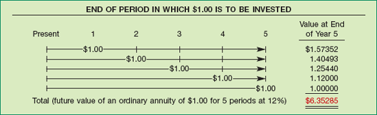
Because an ordinary annuity consists of rents deposited at the end of the period, those rents earn no interest during the period. For example, the third rent earns interest for only two periods (periods four and five). It earns no interest for the third period since it is not deposited until the end of the third period. When computing the future value of an ordinary annuity, the number of compounding periods will always be one less than the number of rents.
The foregoing procedure for computing the future value of an ordinary annuity always produces the correct answer. However, it can become cumbersome if the number of rents is large. A formula provides a more efficient way of expressing the future value of an ordinary annuity of 1. This formula sums the individual rents plus the compound interest, as follows:
where
| FVF-OAn,i = future value factor of an ordinary annuity |
| i = rate of interest per period |
| n = number of compounding periods |
For example, FVF-OA5,12% refers to the value to which an ordinary annuity of 1 will accumulate in 5 periods at 12% interest.
Using the formula above has resulted in the development of tables, similar to those used for the "future value of 1" and the "present value of 1" for both an ordinary annuity and an annuity due. Illustration 6-18 provides an excerpt from the "future value of an ordinary annuity of 1" table.
Interpreting the table, if $1 is invested at the end of each year for 4 years at 11% interest compounded annually, the value of the annuity at the end of the fourth year is $4.71 (4.70973 × $1.00). Now, multiply the factor from the appropriate line and column of the table by the dollar amount of one rent involved in an ordinary annuity. The result: the accumulated sum of the rents and the compound interest to the date of the last rent.
The following formula computes the future value of an ordinary annuity.
where
| R = periodic rent |
| FVF-OAn,i = future value of an ordinary annuity factor for n periods at i interest |
To illustrate, what is the future value of five $5,000 deposits made at the end of each of the next 5 years, earning interest of 12%? Illustration 6-19 depicts this problem as a time diagram.
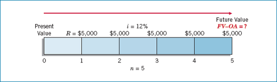
Use of the formula solves this investment problem as follows.
To determine the future value of an ordinary annuity factor of 6.35285 in the formula above, use a financial calculator or read the appropriate table, in this case, Table 6-3 (12% column and the 5-period row).
To illustrate these computations in a business situation, assume that Hightown Electronics deposits $75,000 at the end of each 6-month period for the next 3 years, to accumulate enough money to meet debts that mature in 3 years. What is the future value that the company will have on deposit at the end of 3 years if the annual interest rate is 10%? The time diagram in Illustration 6-20 depicts this situation.
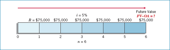
The formula solution for the Hightown Electronics situation is as follows.
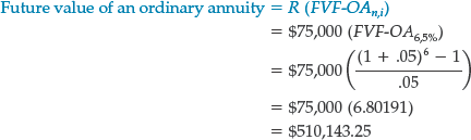
Thus, six 6-month deposits of $75,000 earning 5% per period will grow to $510,143.25.
The preceding analysis of an ordinary annuity assumed that the periodic rents occur at the end of each period. Recall that an annuity due assumes periodic rents occur at the beginning of each period. This means an annuity due will accumulate interest during the first period (in contrast to an ordinary annuity rent, which will not). In other words, the two types of annuities differ in the number of interest accumulation periods involved.
If rents occur at the end of a period (ordinary annuity), in determining the future value of an annuity there will be one less interest period than if the rents occur at the beginning of the period (annuity due). Illustration 6-21 shows this distinction.
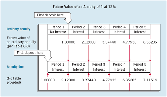
In this example, the cash flows from the annuity due come exactly one period earlier than for an ordinary annuity. As a result, the future value of the annuity due factor is exactly 12% higher than the ordinary annuity factor. For example, the value of an ordinary annuity factor at the end of period one at 12% is 1.00000, whereas for an annuity due it is 1.12000.
To find the future value of an annuity due factor, multiply the future value of an ordinary annuity factor by 1 plus the interest rate. For example, to determine the future value of an annuity due interest factor for 5 periods at 12% compound interest, simply multiply the future value of an ordinary annuity interest factor for 5 periods (6.35285), by one plus the interest rate (1 + .12), to arrive at 7.11519 (6.35285 × 1.12).
To illustrate the use of the ordinary annuity tables in converting to an annuity due, assume that Sue Lotadough plans to deposit $800 a year on each birthday of her son Howard. She makes the first deposit on his tenth birthday, at 6% interest compounded annually. Sue wants to know the amount she will have accumulated for college expenses by her son's eighteenth birthday.
If the first deposit occurs on Howard's tenth birthday, Sue will make a total of 8 deposits over the life of the annuity (assume no deposit on the eighteenth birthday), as shown in Illustration 6-22. Because all the deposits are made at the beginning of the periods, they represent an annuity due.

Referring to the "future value of an ordinary annuity of 1" table for 8 periods at 6%, Sue finds a factor of 9.89747. She then multiplies this factor by (1 + .06) to arrive at the future value of an annuity due factor. As a result, the accumulated value on Howard's eighteenth birthday is $8,393.05, as calculated in Illustration 6-23.
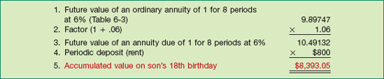
Depending on the college he chooses, Howard may have enough to finance only part of his first year of school.
The foregoing annuity examples relied on three known values—amount of each rent, interest rate, and number of periods. Using these values enables us to determine the unknown fourth value, future value.
The first two future value problems we present illustrate the computations of (1) the amount of the rents and (2) the number of rents. The third problem illustrates the computation of the future value of an annuity due.
Assume that you plan to accumulate $14,000 for a down payment on a condominium apartment 5 years from now. For the next 5 years, you earn an annual return of 8% compounded semiannually. How much should you deposit at the end of each 6-month period?
The $14,000 is the future value of 10 (5 × 2) semiannual end-of-period payments of an unknown amount, at an interest rate of 4% (8% ÷ 2). Illustration 6-24 depicts this problem as a time diagram.
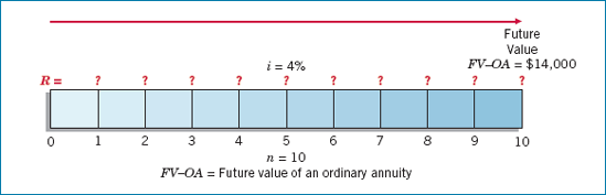
Using the formula for the future value of an ordinary annuity, you determine the amount of each rent as follows.
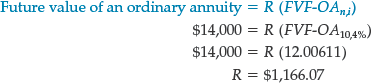
Thus, you must make 10 semiannual deposits of $1,166.07 each in order to accumulate $14,000 for your down payment.
Suppose that a company's goal is to accumulate $117,332 by making periodic deposits of $20,000 at the end of each year, which will earn 8% compounded annually while accumulating. How many deposits must it make?
The $117,332 represents the future value of n (?) $20,000 deposits, at an 8% annual rate of interest. Illustration 6-25 depicts this problem in a time diagram.
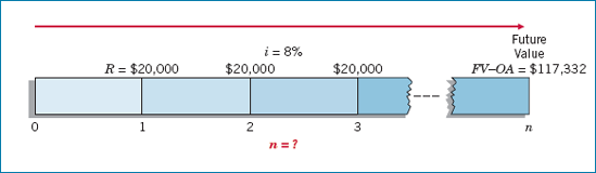
Using the future value of an ordinary annuity formula, the company obtains the following factor.
Use Table 6-3 and read down the 8% column to find 5.86660 in the 5-period row. Thus, the company must make five deposits of $20,000 each.
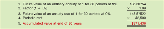
To create his retirement fund, Walter Goodwrench, a mechanic, now works weekends. Mr. Goodwrench deposits $2,500 today in a savings account that earns 9% interest. He plans to deposit $2,500 every year for a total of 30 years. How much cash will Mr. Goodwrench accumulate in his retirement savings account, when he retires in 30 years? Illustration 6-26 depicts this problem in a time diagram.
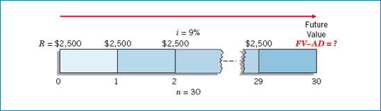
Using the "future value of an ordinary annuity of 1" table, Mr. Goodwrench computes the solution as shown in Illustration 6-27.
The present value of an annuity is the single sum that, if invested at compound interest now, would provide for an annuity (a series of withdrawals) for a certain number of future periods. In other words, the present value of an ordinary annuity is the present value of a series of equal rents, to withdraw at equal intervals.
One approach to finding the present value of an annuity determines the present value of each of the rents in the series and then totals their individual present values. For example, we may view an annuity of $1, to be received at the end of each of 5 periods, as separate amounts. We then compute each present value using the table of present values (see pages 310–311), assuming an interest rate of 12%. Illustration 6-28 shows this approach.
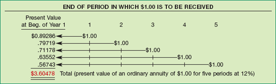
This computation tells us that if we invest the single sum of $3.60 today at 12% interest for 5 periods, we will be able to withdraw $1 at the end of each period for 5 periods. We can summarize this cumbersome procedure by the following formula.
The expression PVF-OAn,i refers to the present value of an ordinary annuity of 1 factor for n periods at i interest. Ordinary annuity tables base present values on this formula. Illustration 6-29 shows an excerpt from such a table.
The general formula for the present value of any ordinary annuity is as follows.
where
| R = periodic rent (ordinary annuity) |
| PVF-OAn,i = present value of an ordinary annuity of 1 for n periods at i interest |
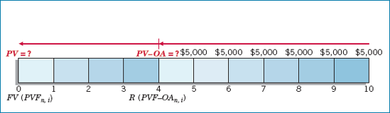
To illustrate with an example, what is the present value of rental receipts of $6,000 each, to be received at the end of each of the next 5 years when discounted at 12%? This problem may be time-diagrammed and solved as shown in Illustration 6-30.
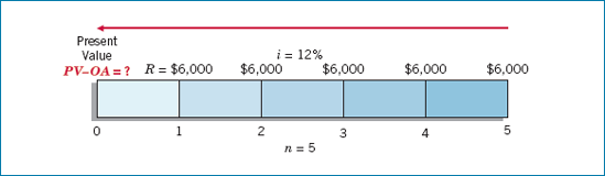
The formula for this calculation is as shown below.
The present value of the 5 ordinary annuity rental receipts of $6,000 each is $21,628.68. To determine the present value of the ordinary annuity factor 3.60478, use a financial calculator or read the appropriate table, in this case Table 6-4 (12% column and 5-period row).
Time value of money concepts also can be relevant to public policy debates. For example, several states had to determine how to receive the payments from tobacco companies as settlement for a national lawsuit against the companies for the healthcare costs of smoking.
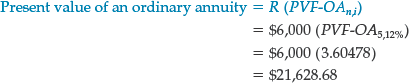
The State of Wisconsin was due to collect 25 years of payments totaling $5.6 billion. The state could wait to collect the payments, or it could sell the payments to an investment bank (a process called securitization). If it were to sell the payments, it would receive a lump-sum payment today of $1.26 billion. Is this a good deal for the state? Assuming a discount rate of 8% and that the payments will be received in equal amounts (e.g., an annuity), the present value of the tobacco payment is:
Why would some in the state be willing to take just $1.26 billion today for an annuity whose present value is almost twice that amount? One reason is that Wisconsin was facing a hole in its budget that could be plugged in part by the lump-sum payment. Also, some believed that the risk of not getting paid by the tobacco companies in the future makes it prudent to get the money earlier.
If this latter reason has merit, then the present value computation above should have been based on a higher interest rate. Assuming a discount rate of 15%, the present value of the annuity is $1.448 billion ($5.6 billion 25 $224 million; $224 million 6.46415), which is much closer to the lump-sum payment offered to the State of Wisconsin.
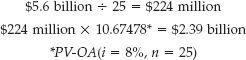
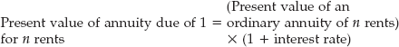
In our discussion of the present value of an ordinary annuity, we discounted the final rent based on the number of rent periods. In determining the present value of an annuity due, there is always one fewer discount period. Illustration 6-31 shows this distinction.
Because each cash flow comes exactly one period sooner in the present value of the annuity due, the present value of the cash flows is exactly 12% higher than the present value of an ordinary annuity. Thus, to find the present value of an annuity due factor, multiply the present value of an ordinary annuity factor by 1 plus the interest rate (that is, 1 + i).
To determine the present value of an annuity due interest factor for 5 periods at 12% interest, take the present value of an ordinary annuity for 5 periods at 12% interest (3.60478) and multiply it by 1.12 to arrive at the present value of an annuity due, 4.03735 (3.60478 × 1.12). We provide present value of annuity due factors in Table 6-5.
To illustrate, Space Odyssey, Inc., rents a communications satellite for 4 years with annual rental payments of $4.8 million to be made at the beginning of each year. If the relevant annual interest rate is 11%, what is the present value of the rental obligations? Illustration 6-32 shows the company's time diagram for this problem.
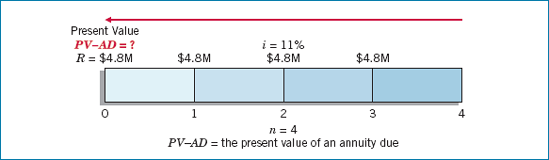
Illustration 6-33 shows the computations to solve this problem.
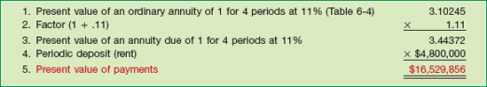
Using Table 6-5 also locates the desired factor 3.44371 and computes the present value of the lease payments to be $16,529,808. (The difference in computations is due to rounding.)
In the following three examples, we demonstrate the computation of (1) the present value, (2) the interest rate, and (3) the amount of each rent.
You have just won a lottery totaling $4,000,000. You learn that you will receive a check in the amount of $200,000 at the end of each of the next 20 years. What amount have you really won? That is, what is the present value of the $200,000 checks you will receive over the next 20 years? Illustration 6-34 (on page 285) shows a time diagram of this enviable situation (assuming an appropriate interest rate of 10%).
You calculate the present value as follows:
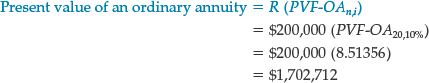
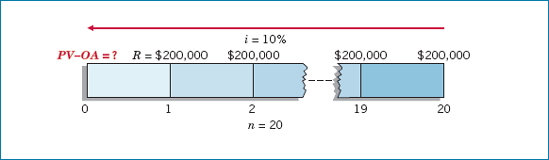
As a result, if the state deposits $1,702,712 now and earns 10% interest, it can withdraw $200,000 a year for 20 years to pay you the $4,000,000.
Many shoppers use credit cards to make purchases. When you receive the statement for payment, you may pay the total amount due or you may pay the balance in a certain number of payments. For example, assume you receive a statement from MasterCard with a balance due of $528.77. You may pay it off in 12 equal monthly payments of $50 each, with the first payment due one month from now. What rate of interest would you be paying?
The $528.77 represents the present value of the 12 payments of $50 each at an unknown rate of interest. The time diagram in Illustration 6-35 depicts this situation.
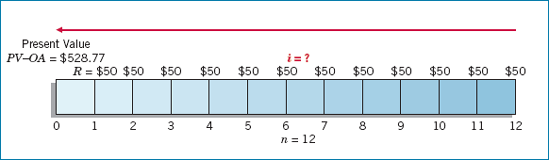
You calculate the rate as follows.
Referring to Table 6-4 and reading across the 12-period row, you find 10.57534 in the 2% column. Since 2% is a monthly rate, the nominal annual rate of interest is 24% (12 × 2%). The effective annual rate is 26.82413% [(1 + .02)12 − 1]. Obviously, you are better off paying the entire bill now if possible.
Norm and Jackie Remmers have saved $36,000 to finance their daughter Dawna's college education. They deposited the money in the Bloomington Savings and Loan Association, where it earns 4% interest compounded semiannually. What equal amounts can their daughter withdraw at the end of every 6 months during her 4 college years, without exhausting the fund? Illustration 6-36 (on page 286) shows a time diagram of this situation.
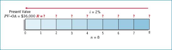
Determining the answer by simply dividing $36,000 by 8 withdrawals is wrong. Why? Because that ignores the interest earned on the money remaining on deposit. Dawna must consider that interest is compounded semiannually at 2% (4% ÷ 2) for 8 periods (4 years × 2). Thus, using the same present value of an ordinary annuity formula, she determines the amount of each withdrawal that she can make as follows.
Solving time value problems often requires using more than one table. For example, a business problem may need computations of both present value of a single sum and present value of an annuity. Two such common situations are:
Deferred annuities.
Bond problems.
A deferred annuity is an annuity in which the rents begin after a specified number of periods. A deferred annuity does not begin to produce rents until two or more periods have expired. For example, "an ordinary annuity of six annual rents deferred 4 years" means that no rents will occur during the first 4 years, and that the first of the six rents will occur at the end of the fifth year. "An annuity due of six annual rents deferred 4 years" means that no rents will occur during the first 4 years, and that the first of six rents will occur at the beginning of the fifth year.
Computing the future value of a deferred annuity is relatively straightforward. Because there is no accumulation or investment on which interest may accrue, the future value of a deferred annuity is the same as the future value of an annuity not deferred. That is, computing the future value simply ignores the deferred period.
To illustrate, assume that Sutton Corporation plans to purchase a land site in 6 years for the construction of its new corporate headquarters. Because of cash flow problems, Sutton budgets deposits of $80,000, on which it expects to earn 5% annually, only at the end of the fourth, fifth, and sixth periods. What future value will Sutton have accumulated at the end of the sixth year? Illustration 6-37 shows a time diagram of this situation.
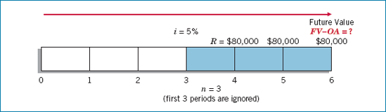
Sutton determines the value accumulated by using the standard formula for the future value of an ordinary annuity:
Computing the present value of a deferred annuity must recognize the interest that accrues on the original investment during the deferral period.
To compute the present value of a deferred annuity, we compute the present value of an ordinary annuity of 1 as if the rents had occurred for the entire period. We then subtract the present value of rents that were not received during the deferral period. We are left with the present value of the rents actually received subsequent to the deferral period.
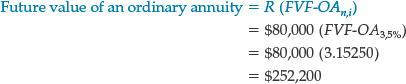
To illustrate, Bob Bender has developed and copyrighted tutorial software for students in advanced accounting. He agrees to sell the copyright to Campus Micro Systems for six annual payments of $5,000 each. The payments will begin 5 years from today. Given an annual interest rate of 8%, what is the present value of the six payments?
This situation is an ordinary annuity of 6 payments deferred 4 periods. The time diagram in Illustration 6-38 depicts this sales agreement.
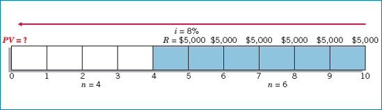
Two options are available to solve this problem. The first is to use only Table 6-4, as shown in Illustration 6-39.
The subtraction of the present value of an annuity of 1 for the deferred periods eliminates the nonexistent rents during the deferral period. It converts the present value of an ordinary annuity of $1.00 for 10 periods to the present value of 6 rents of $1.00, deferred 4 periods.
Alternatively, Bender can use both Table 6-2 and Table 6-4 to compute the present value of the 6 rents. He can first discount the annuity 6 periods. However, because the annuity is deferred 4 periods, he must treat the present value of the annuity as a future amount to be discounted another 4 periods. The time diagram in Illustration 6-40 depicts this two-step process.
Calculation using formulas would be done in two steps, as follows.
The present value of $16,989.78 computed above is the same as in Illustration 6-39, although computed differently. (The $0.03 difference is due to rounding.)
A long-term bond produces two cash flows: (1) periodic interest payments during the life of the bond, and (2) the principal (face value) paid at maturity. At the date of issue, bond buyers determine the present value of these two cash flows using the market rate of interest.
The periodic interest payments represent an annuity. The principal represents a single-sum problem. The current market value of the bonds is the combined present values of the interest annuity and the principal amount.
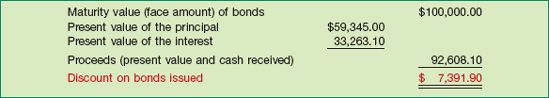
To illustrate, Alltech Corporation on January 1, 2010, issues $100,000 of 9% bonds due in 5 years with interest payable annually at year-end. The current market rate of interest for bonds of similar risk is 11%. What will the buyers pay for this bond issue?
The time diagram in Illustration 6-41 depicts both cash flows.
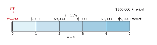
Alltech computes the present value of the two cash flows by discounting at 11% as follows.
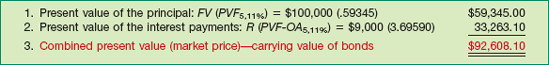
By paying $92,608.10 at date of issue, the buyers of the bonds will realize an effective yield of 11% over the 5-year term of the bonds. This is true because Alltech discounted the cash flows at 11%.
In the previous example (Illustration 6-42), Alltech Corporation issued bonds at a discount, computed as follows.
Alltech amortizes (writes off to interest expense) the amount of this discount over the life of the bond issue.
The preferred procedure for amortization of a discount or premium is the effective-interest method. Under the effective-interest method:
The company issuing the bond first computes bond interest expense by multiplying the carrying value of the bonds at the beginning of the period by the effective interest rate.
The company then determines the bond discount or premium amortization by comparing the bond interest expense with the interest to be paid.
Illustration 6-44 depicts the computation of bond amortization.
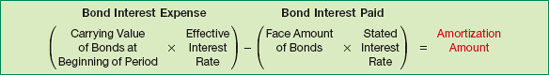
The effective-interest method produces a periodic interest expense equal to a constant percentage of the carrying value of the bonds. Since the percentage used is the effective rate of interest incurred by the borrower at the time of issuance, the effective-interest method results in matching expenses with revenues.
We can use the data from the Alltech Corporation example to illustrate the effective-interest method of amortization. Alltech issued $100,000 face value of bonds at a discount of $7,391.90, resulting in a carrying value of $92,608.10. Illustration 6-45 shows the effective-interest amortization schedule for Alltech's bonds.
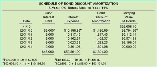
We use the amortization schedule illustrated above for note and bond transactions in Chapters 7 and 14.
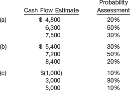
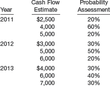
In the past, most accounting calculations of present value relied on the most likely cash flow amount. Concepts Statement No. 7 introduces an expected cash flow approach.[78] It uses a range of cash flows and incorporates the probabilities of those cash flows to provide a more relevant measurement of present value.
To illustrate the expected cash flow model, assume that there is a 30% probability that future cash flows will be $100, a 50% probability that they will be $200, and a 20% probability that they will be $300. In this case, the expected cash flow would be $190 [($100 × 0.3) + ($200 × 0.5) + ($300 × 0.2)]. Traditional present value approaches would use the most likely estimate ($200). However, that estimate fails to consider the different probabilities of the possible cash flows.
Management of the level of interest rates is an important policy tool of the Federal Reserve Bank and its chair, Ben Bernanke. Through a number of policy options, the Fed has the ability to move interest rates up or down, and these rate changes can affect the wealth of all market participants. For example, if the Fed wants to raise rates (because the overall economy is getting overheated), it can raise the discount rate, which is the rate banks pay to borrow money from the Fed. This rate increase will factor into the rates banks and other creditors use to lend money. As a result, companies will think twice about borrowing money to expand their businesses. The result will be a slowing economy. A rate cut does just the opposite: It makes borrowing cheaper, and it can help the economy expand as more companies borrow to expand their operations.
Keeping rates low had been the Fed's policy for much of the early years of this decade. The low rates did help keep the economy humming. But these same low rates may have also resulted in too much real estate lending and the growth of a real estate bubble, as the price of housing was fueled by cheaper low-interest mortgage loans. But, as the old saying goes, "What goes up, must come down." That is what real estate prices did, triggering massive loan write-offs, a seizing up of credit markets, and a slowing economy.
So just when a rate cut might help the economy, the Fed's rate-cutting toolbox is empty. As a result, the Fed began to explore other options, such as loan guarantees, to help banks lend more money and to spur the economy out of its recent funk.
Source: J. Lahart, "Fed Might Need to Reload," Wall Street Journal (March 27, 2008), p. A6.
After determining expected cash flows, a company must then use the proper interest rate to discount the cash flows. The interest rate used for this purpose has three components:
The FASB takes the position that after computing the expected cash flows, a company should discount those cash flows by the risk-free rate of return. That rate is defined as the pure rate of return plus the expected inflation rate. The Board notes that the expected cash flow framework adjusts for credit risk because it incorporates the probability of receipt or payment into the computation of expected cash flows. Therefore, the rate used to discount the expected cash flows should consider only the pure rate of interest and the inflation rate.
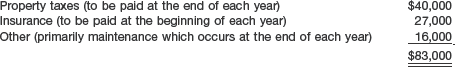
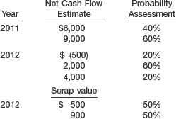
To illustrate, assume that Al's Appliance Outlet offers a 2-year warranty on all products sold. In 2010 Al's Appliance sold $250,000 of a particular type of clothes dryer. Al's Appliance entered into an agreement with Ralph's Repair to provide all warranty service on the dryers sold in 2010. To determine the warranty expense to record in 2010 and the amount of warranty liability to record on the December 31, 2010, balance sheet, Al's Appliance must measure the fair value of the agreement. Since there is not a ready market for these warranty contracts, Al's Appliance uses expected cash flow techniques to value the warranty obligation.
Based on prior warranty experience, Al's Appliance estimates the expected cash outflows associated with the dryers sold in 2010, as shown in Illustration 6-46.
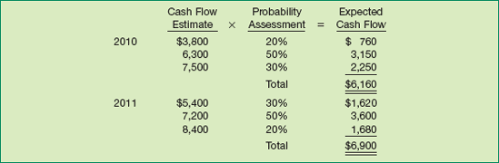
Applying expected cash flow concepts to these data, Al's Appliance estimates warranty cash outflows of $6,160 in 2010 and $6,900 in 2011.
Illustration 6-47 shows the present value of these cash flows, assuming a risk-free rate of 5 percent and cash flows occurring at the end of the year.

FUNDAMENTAL CONCEPTS
SIMPLE INTEREST. Interest on principal only, regardless of interest that may have accrued in the past.
COMPOUND INTEREST. Interest accrues on the unpaid interest of past periods as well as on the principal.
RATE OF INTEREST. Interest is usually expressed as an annual rate, but when the compounding period is shorter than one year, the interest rate for the shorter period must be determined.
ANNUITY. A series of payments or receipts (called rents) that occur at equal intervals of time. Types of annuities:
Ordinary Annuity. Each rent is payable (receivable) at the end of the period.
Annuity Due. Each rent is payable (receivable) at the beginning of the period.
FUTURE VALUE. Value at a later date of a single sum that is invested at compound interest.
Future Value of 1 (or value of a single sum). The future value of $1 (or a single given sum), FV, at the end of n periods at i compound interest rate (Table 6-1).
Future Value of an Annuity. The future value of a series of rents invested at compound interest. In other words, the accumulated total that results from a series of equal deposits at regular intervals invested at compound interest. Both deposits and interest increase the accumulation.
PRESENT VALUE. The value at an earlier date (usually now) of a given future sum discounted at compound interest.
Present Value of 1 (or present value of a single sum). The present value (worth) of $1 (or a given sum), due n periods hence, discounted at i compound interest (Table 6-2).
Present Value of an Annuity. The present value (worth) of a series of rents discounted at compound interest. In other words, it is the sum when invested at compound interest that will permit a series of equal withdrawals at regular intervals.
Present Value of an Ordinary Annuity. The value now of $1 to be received or paid at the end of each period (rents) for n periods, discounted at i compound interest (Table 6-4).
Present Value of an Annuity Due. The value now of $1 to be received or paid at the beginning of each period (rents) for n periods, discounted at i compound interest (Table 6-5). To use Table 4 for an annuity due, apply this formula.
FASB Codification References
FASB ASC 820-10. [Predecessor literature: "Fair Value Measurement," Statement of Financial Accounting Standards No. 157 (Norwalk, Conn.: FASB, September 2006).]
FASB ASC 310-10. [Predecessor literature: "Accounting by Creditors for Impairment of a Loan," FASB Statement No. 114 (Norwalk, Conn.: FASB, May 1993).]
FASB ASC 840-30-30. [Predecessor literature: "Accounting for Leases," FASB Statement No. 13 as amended and interpreted through May 1980 (Stamford, Conn.: FASB, 1980).]
FASB ASC 715-30-35. [Predecessor literature: "Employers' Accounting for Pension Plans," Statement of Financial Accounting Standards No. 87 (Stamford, Conn.: FASB, 1985).]
FASB ASC 360-10-35. [Predecessor literature: "Accounting for the Impairment or Disposal of Long-Lived Assets," Statement of Financial Accounting Standards No. 144 (Norwalk, Conn.: FASB, 2001).]
FASB ASC 718-10-10. [Predecessor literature: "Accounting for Stock-Based Compensation," Statement of Financial Accounting Standards No. 123 (Norwalk, Conn: FASB, 1995); and "Share-Based Payment," Statement of Financial Accounting Standard No. 123(R) (Norwalk, Conn: FASB, 2004).]
What is the time value of money? Why should accountants have an understanding of compound interest, annuities, and present value concepts?
Identify three situations in which accounting measures are based on present values. Do these present value applications involve single sums or annuities, or both single sums and annuities? Explain.
What is the nature of interest? Distinguish between "simple interest" and "compound interest."
What are the components of an interest rate? Why is it important for accountants to understand these components?
Presented below are a number of values taken from compound interest tables involving the same number of periods and the same rate of interest. Indicate what each of these four values represents.
6.71008
2.15892
.46319
14.48656
Jose Oliva is considering two investment options for a $1,500 gift he received for graduation. Both investments have 8% annual interest rates. One offers quarterly compounding; the other compounds on a semiannual basis. Which investment should he choose? Why?
Regina Henry deposited $20,000 in a money market certificate that provides interest of 10% compounded quarterly if the amount is maintained for 3 years. How much will Regina Henry have at the end of 3 years?
Will Smith will receive $80,000 on December 31, 2015 (5 years from now) from a trust fund established by his father. Assuming the appropriate interest rate for discounting is 12% (compounded semiannually), what is the present value of this amount today?
What are the primary characteristics of an annuity? Differentiate between an "ordinary annuity" and an "annuity due."
Kehoe, Inc. owes $40,000 to Ritter Company. How much would Kehoe have to pay each year if the debt is retired through four equal payments (made at the end of the year), given an interest rate on the debt of 12%? (Round to two decimal places.)
The Kellys are planning for a retirement home. They estimate they will need $200,000 4 years from now to purchase this home. Assuming an interest rate of 10%, what amount must be deposited at the end of each of the 4 years to fund the home price? (Round to two decimal places.)
Assume the same situation as in Question 11, except that the four equal amounts are deposited at the beginning of the period rather than at the end. In this case, what amount must be deposited at the beginning of each period? (Round to two decimals.)
Explain how the future value of an ordinary annuity interest table is converted to the future value of an annuity due interest table.
Explain how the present value of an ordinary annuity interest table is converted to the present value of an annuity due interest table.
In a book named Treasure, the reader has to figure out where a 2.2 pound, 24 kt gold horse has been buried. If the horse is found, a prize of $25,000 a year for 20 years is provided. The actual cost to the publisher to purchase an annuity to pay for the prize is $245,000. What interest rate (to the nearest percent) was used to determine the amount of the annuity? (Assume end-of-year payments.)
Alexander Enterprises leases property to Hamilton, Inc. Because Hamilton, Inc. is experiencing financial difficulty, Alexander agrees to receive five rents of $20,000 at the end of each year, with the rents deferred 3 years. What is the present value of the five rents discounted at 12%?
Answer the following questions.
On May 1, 2010, Goldberg Company sold some machinery to Newlin Company on an installment contract basis. The contract required five equal annual payments, with the first payment due on May 1, 2010. What present value concept is appropriate for this situation?
On June 1, 2010, Seymour Inc. purchased a new machine that it does not have to pay for until May 1, 2012. The total payment on May 1, 2012, will include both principal and interest. Assuming interest at a 12% rate, the cost of the machine would be the total payment multiplied by what time value of money concept?
Costner Inc. wishes to know how much money it will have available in 5 years if five equal amounts of $35,000 are invested, with the first amount invested immediately. What interest table is appropriate for this situation?
Jane Hoffman invests in a "jumbo" $200,000, 3-year certificate of deposit at First Wisconsin Bank. What table would be used to determine the amount accumulated at the end of 3 years?
Recently Glenda Estes was interested in purchasing a Honda Acura. The salesperson indicated that the price of the car was either $27,600 cash or $6,900 at the end of each of 5 years. Compute the effective interest rate to the nearest percent that Glenda would pay if she chooses to make the five annual payments.
Recently, property/casualty insurance companies have been criticized because they reserve for the total loss as much as 5 years before it may happen. The IRS has joined the debate because they say the full reserve is unfair from a taxation viewpoint. What do you believe is the IRS position?
(Interest rates are per annum unless otherwise indicated.)

In a future value of 1 table
In a present value of an annuity of 1 table


Instructions
Compute the amount Lyle would withdraw assuming the investment earns simple interest.
Compute the amount Lyle would withdraw assuming the investment earns interest compounded annually.
Compute the amount Lyle would withdraw assuming the investment earns interest compounded semiannually.

What is the future value of $9,000 at the end of 5 periods at 8% compounded interest?
What is the present value of $9,000 due 8 periods hence, discounted at 11%?
What is the future value of 15 periodic payments of $9,000 each made at the end of each period and compounded at 10%?
What is the present value of $9,000 to be received at the end of each of 20 periods, discounted at 5% compound interest?

What is the future value of 20 periodic payments of $5,000 each made at the beginning of each period and compounded at 8%?
What is the present value of $2,500 to be received at the beginning of each of 30 periods, discounted at 10% compound interest?
What is the future value of 15 deposits of $2,000 each made at the beginning of each period and compounded at 10%? (Future value as of the end of the fifteenth period.)
What is the present value of six receipts of $3,000 each received at the beginning of each period, discounted at 9% compounded interest?
$50,000 receivable at the end of each period for 8 periods compounded at 12%.
$50,000 payments to be made at the end of each period for 16 periods at 9%.
$50,000 payable at the end of the seventh, eighth, ninth, and tenth periods at 12%.
Ron Stein Company recently signed a lease for a new office building, for a lease period of 10 years. Under the lease agreement, a security deposit of $12,000 is made, with the deposit to be returned at the expiration of the lease, with interest compounded at 10% per year. What amount will the company receive at the time the lease expires?
Kate Greenway Corporation, having recently issued a $20 million, 15-year bond issue, is committed to make annual sinking fund deposits of $620,000. The deposits are made on the last day of each year and yield a return of 10%. Will the fund at the end of 15 years be sufficient to retire the bonds? If not, what will the deficiency be?
Under the terms of his salary agreement, president Juan Rivera has an option of receiving either an immediate bonus of $40,000, or a deferred bonus of $75,000 payable in 10 years. Ignoring tax considerations, and assuming a relevant interest rate of 8%, which form of settlement should Rivera accept?

8%?
10%?
12%?
Instructions
How much must the balance of the fund equal on June 30, 2013, in order for Stephen Bosworth to satisfy his objective?
What are each of Stephen's contributions to the fund?
Mark Yoders wishes to become a millionaire. His money market fund has a balance of $148,644 and has a guaranteed interest rate of 10%. How many years must Mark leave that balance in the fund in order to get his desired $1,000,000?
Assume that Elvira Lehman desires to accumulate $1 million in 15 years using her money market fund balance of $239,392. At what interest rate must Elvira's investment compound annually?

Instructions
How much total interest will Amos pay on this payment plan?
Amos could borrow $100,000 from its bank to finance the purchase at an annual rate of 8%. Should Amos borrow from the bank or use the manufacturer's payment plan to pay for the equipment?
Building A: Purchase for a cash price of $610,000, useful life 25 years.
Building B: Lease for 25 years with annual lease payments of $70,000 being made at the beginning of the year.
Building C: Purchase for $650,000 cash. This building is larger than needed; however, the excess space can be sublet for 25 years at a net annual rental of $6,000. Rental payments will be received at the end of each year. Brubaker Inc. has no aversion to being a landlord.
Instructions
In which building would you recommend that Brubaker Inc. locate, assuming a 12% cost of funds?
Instructions
As the controller of the company, determine the selling price of the bonds.
Average length of time to retirement
15 years
Expected life duration after retirement
10 years
Total pension payment expected each year after retirement for all employees. Payment made at the end of the year.
$800,000 per year
The interest rate to be used is 8%.
Instructions
On the basis of the information above, determine the present value of the pension liability.
Instructions
If Lee plans to establish the DL Foundation once the fund grows to $1,898,000, how many years until he can establish the foundation?
Instead of investing the entire $1,000,000, Lee invests $300,000 today and plans to make 9 equal annual investments into the fund beginning one year from today. What amount should the payments be if Lee plans to establish the $1,898,000 foundation at the end of 9 years?
Instructions
How much must be contributed each year by Alex Hardaway to provide a fund sufficient to retire the debt on March 1, 2018?
Instructions
You are requested to provide Wyeth with the amount of each of the 25 rental payments that will yield an 11% return on investment.
Instructions
Which method of payment do you recommend, assuming an expected effective interest rate of 8% during the future period?

Engine Overhaul Estimated Cash Outflow
Probability Assessment
$200
10%
450
30%
600
50%
750
10%
Instructions
How much should Keith Bowie deposit today in an account earning 6%, compounded annually, so that he will have enough money on hand in 2 years to pay for the overhaul?
Cash Flow Estimate
Probability Assessment
$380,000
20%
630,000
50%
750,000
30%
Instructions
What is the estimated fair value of the trade name? Killroy determines that the appropriate discount rate for this estimation is 8%. Round calculations to the nearest dollar.
Is the estimate developed for part (a) a Level 1 or Level 3 fair value estimate? Explain.
(Interest rates are per annum unless otherwise indicated.)

On January 1, 2010, Fishbone Corporation purchased 300 of the $1,000 face value, 9%, 10-year bonds of Walters Inc. The bonds mature on January 1, 2020, and pay interest annually beginning January 1, 2011. Fishbone purchased the bonds to yield 11%. How much did Fishbone pay for the bonds?
Fishbone Corporation bought a new machine and agreed to pay for it in equal annual installments of $4,000 at the end of each of the next 10 years. Assuming that a prevailing interest rate of 8% applies to this contract, how much should Fishbone record as the cost of the machine?
Fishbone Corporation purchased a special tractor on December 31, 2010. The purchase agreement stipulated that Fishbone should pay $20,000 at the time of purchase and $5,000 at the end of each of the next 8 years. The tractor should be recorded on December 31, 2010, at what amount, assuming an appropriate interest rate of 12%?
Fishbone Corporation wants to withdraw $120,000 (including principal) from an investment fund at the end of each year for 9 years. What should be the required initial investment at the beginning of the first year if the fund earns 11%?
Diane Ross has $20,000 to invest today at 9% to pay a debt of $47,347. How many years will it take her to accumulate enough to liquidate the debt?
Cindy Houston has a $27,600 debt that she wishes to repay 4 years from today; she has $19,553 that she intends to invest for the 4 years. What rate of interest will she need to earn annually in order to accumulate enough to pay the debt?
Bid A: A surface that costs $5.75 per square yard to install. This surface will have to be replaced at the end of 5 years. The annual maintenance cost on this surface is estimated at 25 cents per square yard for each year except the last year of its service. The replacement surface will be similar to the initial surface.
Bid B: A surface that costs $10.50 per square yard to install. This surface has a probable useful life of 10 years and will require annual maintenance in each year except the last year, at an estimated cost of 9 cents per square yard.
Instructions
Prepare computations showing which bid should be accepted by Wal-Mart, Inc. You may assume that the cost of capital is 9%, that the annual maintenance expenditures are incurred at the end of each year, and that prices are not expected to change during the next 10 years.
Instructions
Assuming Howie can earn an 8% rate of return (compounded annually) on any money invested during this period, which pay-out option should he choose?
$55,000 immediate cash.
$4,000 every 3 months payable at the end of each quarter for 5 years.
$18,000 immediate cash and $1,800 every 3 months for 10 years, payable at the beginning of each 3-month period.
$4,000 every 3 months for 3 years and $1,500 each quarter for the following 25 quarters, all payments payable at the end of each quarter.
Instructions
If money is worth 2½% per quarter, compounded quarterly, which option would you recommend that Brent exercise?
The vineyard will bear no grapes for the first 5 years (1–5). In the next 5 years (6–10), Stacy estimates that the vines will bear grapes that can be sold for $60,000 each year. For the next 20 years (11–30) she expects the harvest will provide annual revenues of $110,000. But during the last 10 years (31–40) of the vineyard's life, she estimates that revenues will decline to $80,000 per year.
During the first 5 years the annual cost of pruning, fertilizing, and caring for the vineyard is estimated at $9,000; during the years of production, 6–40, these costs will rise to $12,000 per year. The relevant market rate of interest for the entire period is 12%. Assume that all receipts and payments are made at the end of each year.
Instructions
Dick Button has offered to buy Stacy's vineyard business by assuming the 40-year lease. On the basis of the current value of the business, what is the minimum price Stacy should accept?
Dubois Inc. has $600,000 to invest. The company is trying to decide between two alternative uses of the funds. One alternative provides $80,000 at the end of each year for 12 years, and the other is to receive a single lump sum payment of $1,900,000 at the end of the 12 years. Which alternative should Dubois select? Assume the interest rate is constant over the entire investment.
Dubois Inc. has completed the purchase of new Dell computers. The fair market value of the equipment is $824,150. The purchase agreement specifies an immediate down payment of $200,000 and semiannual payments of $76,952 beginning at the end of 6 months for 5 years. What is the interest rate, to the nearest percent, used in discounting this purchase transaction?
Dubois Inc. loans money to John Kruk Corporation in the amount of $800,000. Dubois accepts an 8% note due in 7 years with interest payable semiannually. After 2 years (and receipt of interest for 2 years), Dubois needs money and therefore sells the note to Chicago National Bank, which demands interest on the note of 10% compounded semiannually. What is the amount Dubois will receive on the sale of the note?
Dubois Inc. wishes to accumulate $1,300,000 by December 31, 2020, to retire bonds outstanding. The company deposits $200,000 on December 31, 2010, which will earn interest at 10% compounded quarterly, to help in the retirement of this debt. In addition, the company wants to know how much should be deposited at the end of each quarter for 10 years to ensure that $1,300,000 is available at the end of 2020. (The quarterly deposits will also earn at a rate of 10%, compounded quarterly.) (Round to even dollars.)
Vendor A: $55,000 cash at time of delivery and 10 year-end payments of $18,000 each. Vendor A offers all its customers the right to purchase at the time of sale a separate 20-year maintenance service contract, under which Vendor A will perform all year-end maintenance at a one-time initial cost of $10,000.
Vendor B: Forty seminannual payments of $9,500 each, with the first installment due upon delivery. Vendor B will perform all year-end maintenance for the next 20 years at no extra charge.
Vendor C: Full cash price of $150,000 will be due upon delivery.
Instructions
Assuming that both Vendor A and B will be able to perform the required year-end maintenance, that Ellison's cost of funds is 10%, and the machine will be purchased on January 1, from which vendor should the press be purchased?
In 2009, McDowell Enterprises negotiated and closed a long-term lease contract for newly constructed truck terminals and freight storage facilities. The buildings were constructed on land owned by the company. On January 1, 2010, McDowell took possession of the leased property. The 20-year lease is effective for the period January 1, 2010, through December 31, 2029. Advance rental payments of $800,000 are payable to the lessor (owner of facilities) on January 1 of each of the first 10 years of the lease term. Advance payments of $400,000 are due on January 1 for each of the last 10 years of the lease term. McDowell has an option to purchase all the leased facilities for $1 on December 31, 2029. At the time the lease was negotiated, the fair market value of the truck terminals and freight storage facilities was approximately $7,200,000. If the company had borrowed the money to purchase the facilities, it would have had to pay 10% interest. Should the company have purchased rather than leased the facilities?
Last year the company exchanged a piece of land for a non-interest-bearing note. The note is to be paid at the rate of $15,000 per year for 9 years, beginning one year from the date of disposal of the land. An appropriate rate of interest for the note was 11%. At the time the land was originally purchased, it cost $90,000. What is the fair value of the note?
The company has always followed the policy to take any cash discounts on goods purchased. Recently the company purchased a large amount of raw materials at a price of $800,000 with terms 1/10, n/30 on which it took the discount. McDowell has recently estimated its cost of funds at 10%. Should McDowell continue this policy of always taking the cash discount?
Purchase: The company can purchase the site, construct the building, and purchase all store fixtures. The cost would be $1,850,000. An immediate down payment of $400,000 is required, and the remaining $1,450,000 would be paid off over 5 years at $350,000 per year (including interest payments made at end of year). The property is expected to have a useful life of 12 years, and then it will be sold for $500,000. As the owner of the property, the company will have the following out-of-pocket expenses each period.
Lease: First National Bank has agreed to purchase the site, construct the building, and install the appropriate fixtures for Dunn Inc. if Dunn will lease the completed facility for 12 years. The annual costs for the lease would be $270,000. Dunn would have no responsibility related to the facility over the 12 years. The terms of the lease are that Dunn would be required to make 12 annual payments (the first payment to be made at the time the store opens and then each following year). In addition, a deposit of $100,000 is required when the store is opened. This deposit will be returned at the end of the twelfth year, assuming no unusual damage to the building structure or fixtures.
Currently the cost of funds for Dunn Inc. is 10%.
Instructions
Which of the two approaches should Dunn Inc. follow?
Jean Honore, owner: Current annual salary of $48,000; estimated retirement date January 1, 2035.
Colin Davis, flower arranger: Current annual salary of $36,000; estimated retirement date January 1, 2040.
Anita Baker, sales clerk: Current annual salary of $18,000; estimated retirement date January 1, 2030.
Gavin Bryars, part-time bookkeeper: Current annual salary of $15,000; estimated retirement date January 1, 2025.
In the past, Jean has given herself and each employee a year-end salary increase of 4%. Jean plans to continue this policy in the future.
Instructions
Based upon the above information, what will be the annual retirement benefit for each plan participant? (Round to the nearest dollar.) (Hint: Jean will receive raises for 24 years.)
What amount must be on deposit at the end of 15 years to ensure that all benefits will be paid? (Round to the nearest dollar.)
What is the amount of each annual deposit Jean must make to the retirement plan?
Under its present plan with First Security, STL is obligated to pay $43 million to meet the expected value of future pension benefits that are payable to employees as an annuity upon their retirement from the company. On the other hand, NET Life requires STL to pay only $35 million for identical future pension benefits. First Security is one of the oldest and most reputable insurance companies in North America. NET Life has a much weaker reputation in the insurance industry. In pondering the significant difference in annual pension costs, Brokaw asks himself, "Is this too good to be true?"
Instructions
Answer the following questions.
Why might NET Life's pension cost requirement be $8 million less than First Security's requirement for the same future value?
What ethical issues should Craig Brokaw consider before switching STL's pension fund assets?
Who are the stakeholders that could be affected by Brokaw's decision?
Using expected cash flow and present value techniques, determine the value of the warranty liability for the 2010 sales. Use an annual discount rate of 5%. Assume all cash flows occur at the end of the year.
Instructions
Using expected cash flow and present value techniques, determine the fair value of the machinery at the end of 2010. Use a 6% discount rate. Assume all cash flows occur at the end of the year.
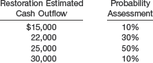
There is no active market for retirement obligations such as these, but Murphy has developed the following cash flow estimates based on its prior experience in mining-site restoration. It will take 3 years to restore the mine site when mining operations cease in 10 years. Each estimated cash outflow reflects an annual payment at the end of each year of the 3-year restoration period.
Instructions
What is the estimated fair value of Murphy's asset retirement obligation? Murphy determines that the appropriate discount rate for this estimation is 5%. Round calculations to the nearest dollar.
Is the estimate developed for part (a) a Level 1 or Level 3 fair value estimate? Explain.
The financial statements and accompanying notes of P&G are presented in Appendix 5B or can be accessed at the book's companion website, www.wiley.com/college/kieso.
Examining each item in P&G's balance sheet, identify those items that require present value, discounting, or interest computations in establishing the amount reported. (The accompanying notes are an additional source for this information.)
(1) What interest rates are disclosed by P&G as being used to compute interest and present values? (2) Why are there so many different interest rates applied to P&G's financial statement elements (assets, liabilities, revenues, and expenses)?
Consolidated Natural Gas Company (CNG), with corporate headquarters in Pittsburgh, Pennsylvania, is one of the largest producers, transporters, distributors, and marketers of natural gas in North America.
Periodically, the company experiences a decrease in the value of its gas and oil producing properties, and a special charge to income was recorded in order to reduce the carrying value of those assets.
Assume the following information: In 2009, CNG estimated the cash inflows from its oil and gas producing properties to be $375,000 per year. During 2010, the write-downs described above caused the estimate to be decreased to $275,000 per year. Production costs (cash outflows) associated with all these properties were estimated to be $125,000 per year in 2009, but this amount was revised to $155,000 per year in 2010.
Instructions
(Assume that all cash flows occur at the end of the year.)
Calculate the present value of net cash flows for 2009–2011 (three years), using the 2009 estimates and a 10% discount factor.
Calculate the present value of net cash flows for 2010–2012 (three years), using the 2010 estimates and a 10% discount factor.
Compare the results using the two estimates. Is information on future cash flows from oil and gas producing properties useful, considering that the estimates must be revised each year? Explain.
At a recent meeting of the accounting staff in your company, the controller raised the issue of using present value techniques to conduct impairment tests for some of the company's fixed assets. Some of the more senior members of the staff admitted having little knowledge of present value concepts in this context, but they had heard about a FASB Concepts Statement that may be relevant. As the junior staff in the department, you have been asked to conduct some research of the authoritative literature on this topic and report back at the staff meeting next week.
Instructions
Access the FASB Statements of Financial Accounting Concepts at the FASB website (http://www.fasb.org) and respond to the following items. (Provide paragraph citations.) When you have accessed the documents, you can search them using the search tool in your Internet browser.
Identify the recent concept statement that addresses present value measurement in accounting.
What are some of the contexts in which present value concepts are applied in accounting measurement?
Provide definitions for the following terms:
Best estimate.
Estimated cash flow (contrasted to expected cash flow).
Fresh-start measurement.
Interest methods of allocation.
Go to the book's companion website, at www.wiley.com/college/kieso, to find an interactive problem that simulates the computerized CPA exam. The professional simulation for this chapter asks you to address questions related to the application of time value of money concepts to accounting problems.
Remember to check the book's companion website to find additional resources for this chapter.
Table 6-1. FUTURE VALUE OF 1 (FUTURE VALUE OF A SINGLE SUM)
FVFn,i = (1 + i)n | |||||||||||||
|---|---|---|---|---|---|---|---|---|---|---|---|---|---|
(n) Periods | 2% | 2½% | 3% | 4% | 5% | 6% | 8% | 9% | 10% | 11% | 12% | 15% | (n) Periods |
1 | 1.02000 | 1.02500 | 1.03000 | 1.04000 | 1.05000 | 1.06000 | 1.08000 | 1.09000 | 1.10000 | 1.11000 | 1.12000 | 1.15000 | 1 |
2 | 1.04040 | 1.05063 | 1.06090 | 1.08160 | 1.10250 | 1.12360 | 1.16640 | 1.18810 | 1.21000 | 1.23210 | 1.25440 | 1.32250 | 2 |
3 | 1.06121 | 1.07689 | 1.09273 | 1.12486 | 1.15763 | 1.19102 | 1.25971 | 1.29503 | 1.33100 | 1.36763 | 1.40493 | 1.52088 | 3 |
4 | 1.08243 | 1.10381 | 1.12551 | 1.16986 | 1.21551 | 1.26248 | 1.36049 | 1.41158 | 1.46410 | 1.51807 | 1.57352 | 1.74901 | 4 |
5 | 1.10408 | 1.13141 | 1.15927 | 1.21665 | 1.27628 | 1.33823 | 1.46933 | 1.53862 | 1.61051 | 1.68506 | 1.76234 | 2.01136 | 5 |
6 | 1.12616 | 1.15969 | 1.19405 | 1.26532 | 1.34010 | 1.41852 | 1.58687 | 1.67710 | 1.77156 | 1.87041 | 1.97382 | 2.31306 | 6 |
7 | 1.14869 | 1.18869 | 1.22987 | 1.31593 | 1.40710 | 1.50363 | 1.71382 | 1.82804 | 1.94872 | 2.07616 | 2.21068 | 2.66002 | 7 |
8 | 1.17166 | 1.21840 | 1.26677 | 1.36857 | 1.47746 | 1.59385 | 1.85093 | 1.99256 | 2.14359 | 2.30454 | 2.47596 | 3.05902 | 8 |
9 | 1.19509 | 1.24886 | 1.30477 | 1.42331 | 1.55133 | 1.68948 | 1.99900 | 2.17189 | 2.35795 | 2.55803 | 2.77308 | 3.51788 | 9 |
10 | 1.21899 | 1.28008 | 1.34392 | 1.48024 | 1.62889 | 1.79085 | 2.15892 | 2.36736 | 2.59374 | 2.83942 | 3.10585 | 4.04556 | 10 |
11 | 1.24337 | 1.31209 | 1.38423 | 1.53945 | 1.71034 | 1.89830 | 2.33164 | 2.58043 | 2.85312 | 3.15176 | 3.47855 | 4.65239 | 11 |
12 | 1.26824 | 1.34489 | 1.42576 | 1.60103 | 1.79586 | 2.01220 | 2.51817 | 2.81267 | 3.13843 | 3.49845 | 3.89598 | 5.35025 | 12 |
13 | 1.29361 | 1.37851 | 1.46853 | 1.66507 | 1.88565 | 2.13293 | 2.71962 | 3.06581 | 3.45227 | 3.88328 | 4.36349 | 6.15279 | 13 |
14 | 1.31948 | 1.41297 | 1.51259 | 1.73168 | 1.97993 | 2.26090 | 2.93719 | 3.34173 | 3.79750 | 4.31044 | 4.88711 | 7.07571 | 14 |
15 | 1.34587 | 1.44830 | 1.55797 | 1.80094 | 2.07893 | 2.39656 | 3.17217 | 3.64248 | 4.17725 | 4.78459 | 5.47357 | 8.13706 | 15 |
16 | 1.37279 | 1.48451 | 1.60471 | 1.87298 | 2.18287 | 2.54035 | 3.42594 | 3.97031 | 4.59497 | 5.31089 | 6.13039 | 9.35762 | 16 |
17 | 1.40024 | 1.52162 | 1.65285 | 1.94790 | 2.29202 | 2.69277 | 3.70002 | 4.32763 | 5.05447 | 5.89509 | 6.86604 | 10.76126 | 17 |
18 | 1.42825 | 1.55966 | 1.70243 | 2.02582 | 2.40662 | 2.85434 | 3.99602 | 4.71712 | 5.55992 | 6.54355 | 7.68997 | 12.37545 | 18 |
19 | 1.45681 | 1.59865 | 1.75351 | 2.10685 | 2.52695 | 3.02560 | 4.31570 | 5.14166 | 6.11591 | 7.26334 | 8.61276 | 14.23177 | 19 |
20 | 1.48595 | 1.63862 | 1.80611 | 2.19112 | 2.65330 | 3.20714 | 4.66096 | 5.60441 | 6.72750 | 8.06231 | 9.64629 | 16.36654 | 20 |
21 | 1.51567 | 1.67958 | 1.86029 | 2.27877 | 2.78596 | 3.39956 | 5.03383 | 6.10881 | 7.40025 | 8.94917 | 10.80385 | 18.82152 | 21 |
22 | 1.54598 | 1.72157 | 1.91610 | 2.36992 | 2.92526 | 3.60354 | 5.43654 | 6.65860 | 8.14028 | 9.93357 | 12.10031 | 21.64475 | 22 |
23 | 1.57690 | 1.76461 | 1.97359 | 2.46472 | 3.07152 | 3.81975 | 5.87146 | 7.25787 | 8.95430 | 11.02627 | 13.55235 | 24.89146 | 23 |
24 | 1.60844 | 1.80873 | 2.03279 | 2.56330 | 3.22510 | 4.04893 | 6.34118 | 7.91108 | 9.84973 | 12.23916 | 15.17863 | 28.62518 | 24 |
25 | 1.64061 | 1.85394 | 2.09378 | 2.66584 | 3.38635 | 4.29187 | 6.84847 | 8.62308 | 10.83471 | 13.58546 | 17.00000 | 32.91895 | 25 |
26 | 1.67342 | 1.90029 | 2.15659 | 2.77247 | 3.55567 | 4.54938 | 7.39635 | 9.39916 | 11.91818 | 15.07986 | 19.04007 | 37.85680 | 26 |
27 | 1.70689 | 1.94780 | 2.22129 | 2.88337 | 3.73346 | 4.82235 | 7.98806 | 10.24508 | 13.10999 | 16.73865 | 21.32488 | 43.53532 | 27 |
28 | 1.74102 | 1.99650 | 2.28793 | 2.99870 | 3.92013 | 5.11169 | 8.62711 | 11.16714 | 14.42099 | 18.57990 | 23.88387 | 50.06561 | 28 |
29 | 1.77584 | 2.04641 | 2.35657 | 3.11865 | 4.11614 | 5.41839 | 9.31727 | 12.17218 | 15.86309 | 20.62369 | 26.74993 | 57.57545 | 29 |
30 | 1.81136 | 2.09757 | 2.42726 | 3.24340 | 4.32194 | 5.74349 | 10.06266 | 13.26768 | 17.44940 | 22.89230 | 29.95992 | 66.21177 | 30 |
31 | 1.84759 | 2.15001 | 2.50008 | 3.37313 | 4.53804 | 6.08810 | 10.86767 | 14.46177 | 19.19434 | 25.41045 | 33.55511 | 76.14354 | 31 |
32 | 1.88454 | 2.20376 | 2.57508 | 3.50806 | 4.76494 | 6.45339 | 11.73708 | 15.76333 | 21.11378 | 28.20560 | 37.58173 | 87.56507 | 32 |
33 | 1.92223 | 2.25885 | 2.65234 | 3.64838 | 5.00319 | 6.84059 | 12.67605 | 17.18203 | 23.22515 | 31.30821 | 42.09153 | 100.69983 | 33 |
34 | 1.96068 | 2.31532 | 2.73191 | 3.79432 | 5.25335 | 7.25103 | 13.69013 | 18.72841 | 25.54767 | 34.75212 | 47.14252 | 115.80480 | 34 |
35 | 1.99989 | 2.37321 | 2.81386 | 3.94609 | 5.51602 | 7.68609 | 14.78534 | 20.41397 | 28.10244 | 38.57485 | 52.79962 | 133.17552 | 35 |
36 | 2.03989 | 2.43254 | 2.89828 | 4.10393 | 5.79182 | 8.14725 | 15.96817 | 22.25123 | 30.91268 | 42.81808 | 59.13557 | 153.15185 | 36 |
37 | 2.08069 | 2.49335 | 2.98523 | 4.26809 | 6.08141 | 8.63609 | 17.24563 | 24.25384 | 34.00395 | 47.52807 | 66.23184 | 176.12463 | 37 |
38 | 2.12230 | 2.55568 | 3.07478 | 4.43881 | 6.38548 | 9.15425 | 18.62528 | 26.43668 | 37.40434 | 52.75616 | 74.17966 | 202.54332 | 38 |
39 | 2.16474 | 2.61957 | 3.16703 | 4.61637 | 6.70475 | 9.70351 | 20.11530 | 28.81598 | 41.14479 | 58.55934 | 83.08122 | 232.92482 | 39 |
40 | 2.20804 | 2.68506 | 3.26204 | 4.80102 | 7.03999 | 10.28572 | 21.72452 | 31.40942 | 45.25926 | 65.00087 | 93.05097 | 267.86355 | 40 |
Table 6-2. PRESENT VALUE OF 1 (PRESENT VALUE OF A SINGLE SUM)
(n) Periods | 2% | 2½% | 3% | 4% | 5% | 6% | 8% | 9% | 10% | 11% | 12% | 15% | (n) Periods |
|---|---|---|---|---|---|---|---|---|---|---|---|---|---|
1 | .98039 | .97561 | .97087 | .96154 | .95238 | .94340 | .92593 | .91743 | .90909 | .90090 | .89286 | .86957 | 1 |
2 | .96117 | .95181 | .94260 | .92456 | .90703 | .89000 | .85734 | .84168 | .82645 | .81162 | .79719 | .75614 | 2 |
3 | .94232 | .92860 | .91514 | .88900 | .86384 | .83962 | .79383 | .77218 | .75132 | .73119 | .71178 | .65752 | 3 |
4 | .92385 | .90595 | .88849 | .85480 | .82270 | .79209 | .73503 | .70843 | .68301 | .65873 | .63552 | .57175 | 4 |
5 | .90573 | .88385 | .86261 | .82193 | .78353 | .74726 | .68058 | .64993 | .62092 | .59345 | .56743 | .49718 | 5 |
6 | .88797 | .86230 | .83748 | .79031 | .74622 | .70496 | .63017 | .59627 | .56447 | .53464 | .50663 | .43233 | 6 |
7 | .87056 | .84127 | .81309 | .75992 | .71068 | .66506 | .58349 | .54703 | .51316 | .48166 | .45235 | .37594 | 7 |
8 | .85349 | .82075 | .78941 | .73069 | .67684 | .62741 | .54027 | .50187 | .46651 | .43393 | .40388 | .32690 | 8 |
9 | .83676 | .80073 | .76642 | .70259 | .64461 | .59190 | .50025 | .46043 | .42410 | .39092 | .36061 | .28426 | 9 |
10 | .82035 | .78120 | .74409 | .67556 | .61391 | .55839 | .46319 | .42241 | .38554 | .35218 | .32197 | .24719 | 10 |
11 | .80426 | .76214 | .72242 | .64958 | .58468 | .52679 | .42888 | .38753 | .35049 | .31728 | .28748 | .21494 | 11 |
12 | .78849 | .74356 | .70138 | .62460 | .55684 | .49697 | .39711 | .35554 | .31863 | .28584 | .25668 | .18691 | 12 |
13 | .77303 | .72542 | .68095 | .60057 | .53032 | .46884 | .36770 | .32618 | .28966 | .25751 | .22917 | .16253 | 13 |
14 | .75788 | .70773 | .66112 | .57748 | .50507 | .44230 | .34046 | .29925 | .26333 | .23199 | .20462 | .14133 | 14 |
15 | .74301 | .69047 | .64186 | .55526 | .48102 | .41727 | .31524 | .27454 | .23939 | .20900 | .18270 | .12289 | 15 |
16 | .72845 | .67362 | .62317 | .53391 | .45811 | .39365 | .29189 | .25187 | .21763 | .18829 | .16312 | .10687 | 16 |
17 | .71416 | .65720 | .60502 | .51337 | .43630 | .37136 | .27027 | .23107 | .19785 | .16963 | .14564 | .09293 | 17 |
18 | .70016 | .64117 | .58739 | .49363 | .41552 | .35034 | .25025 | .21199 | .17986 | .15282 | .13004 | .08081 | 18 |
19 | .68643 | .62553 | .57029 | .47464 | .39573 | .33051 | .23171 | .19449 | .16351 | .13768 | .11611 | .07027 | 19 |
20 | .67297 | .61027 | .55368 | .45639 | .37689 | .31180 | .21455 | .17843 | .14864 | .12403 | .10367 | .06110 | 20 |
21 | .65978 | .59539 | .53755 | .43883 | .35894 | .29416 | .19866 | .16370 | .13513 | .11174 | .09256 | .05313 | 21 |
22 | .64684 | .58086 | .52189 | .42196 | .34185 | .22751 | .18394 | .15018 | .12285 | .10067 | .08264 | .04620 | 22 |
23 | .63416 | .56670 | .50669 | .40573 | .32557 | .26180 | .17032 | .13778 | .11168 | .09069 | .07379 | .04017 | 23 |
24 | .62172 | .55288 | .49193 | .39012 | .31007 | .24698 | .15770 | .12641 | .10153 | .08170 | .06588 | .03493 | 24 |
25 | .60953 | .53939 | .47761 | .37512 | .29530 | .23300 | .14602 | .11597 | .09230 | .07361 | .05882 | .03038 | 25 |
26 | .59758 | .52623 | .46369 | .36069 | .28124 | .21981 | .13520 | .10639 | .08391 | .06631 | .05252 | .02642 | 26 |
27 | .58586 | .51340 | .45019 | .34682 | .26785 | .20737 | .12519 | .09761 | .07628 | .05974 | .04689 | .02297 | 27 |
28 | .57437 | .50088 | .43708 | .33348 | .25509 | .19563 | .11591 | .08955 | .06934 | .05382 | .04187 | .01997 | 28 |
29 | .56311 | .48866 | .42435 | .32065 | .24295 | .18456 | .10733 | .08216 | .06304 | .04849 | .03738 | .01737 | 29 |
30 | .55207 | .47674 | .41199 | .30832 | .23138 | .17411 | .09938 | .07537 | .05731 | .04368 | .03338 | .01510 | 30 |
31 | .54125 | .46511 | .39999 | .29646 | .22036 | .16425 | .09202 | .06915 | .05210 | .03935 | .02980 | .01313 | 31 |
32 | .53063 | .45377 | .38834 | .28506 | .20987 | .15496 | .08520 | .06344 | .04736 | .03545 | .02661 | .01142 | 32 |
33 | .52023 | .44270 | .37703 | .27409 | .19987 | .14619 | .07889 | .05820 | .04306 | .03194 | .02376 | .00993 | 33 |
34 | .51003 | .43191 | .36604 | .26355 | .19035 | .13791 | .07305 | .05340 | .03914 | .02878 | .02121 | .00864 | 34 |
35 | .50003 | .42137 | .35538 | .25342 | .18129 | .13011 | .06763 | .04899 | .03558 | .02592 | .01894 | .00751 | 35 |
36 | .49022 | .41109 | .34503 | .24367 | .17266 | .12274 | .06262 | .04494 | .03235 | .02335 | .01691 | .00653 | 36 |
37 | .48061 | .40107 | .33498 | .23430 | .16444 | .11579 | .05799 | .04123 | .02941 | .02104 | .01510 | .00568 | 37 |
38 | .47119 | .39128 | .32523 | .22529 | .15661 | .10924 | .05369 | .03783 | .02674 | .01896 | .01348 | .00494 | 38 |
39 | .46195 | .38174 | .31575 | .21662 | .14915 | .10306 | .04971 | .03470 | .02430 | .01708 | .01204 | .00429 | 39 |
40 | .45289 | .37243 | .30656 | .20829 | .14205 | .09722 | .04603 | .03184 | .02210 | .01538 | .01075 | .00373 | 40 |
Table 6-3. FUTURE VALUE OF AN ORDINARY ANNUITY OF 1
(n) Periods | 2% | 2½% | 3% | 4% | 5% | 6% | 8% | 9% | 10% | 11% | 12% | 15% | (n) Periods |
|---|---|---|---|---|---|---|---|---|---|---|---|---|---|
1 | 1.00000 | 1.00000 | 1.00000 | 1.00000 | 1.00000 | 1.00000 | 1.00000 | 1.00000 | 1.00000 | 1.00000 | 1.00000 | 1.00000 | 1 |
2 | 2.02000 | 2.02500 | 2.03000 | 2.04000 | 2.05000 | 2.06000 | 2.08000 | 2.09000 | 2.10000 | 2.11000 | 2.12000 | 2.15000 | 2 |
3 | 3.06040 | 3.07563 | 3.09090 | 3.12160 | 3.15250 | 3.18360 | 3.24640 | 3.27810 | 3.31000 | 3.34210 | 3.37440 | 3.47250 | 3 |
4 | 4.12161 | 4.15252 | 4.18363 | 4.24646 | 4.31013 | 4.37462 | 4.50611 | 4.57313 | 4.64100 | 4.70973 | 4.77933 | 4.99338 | 4 |
5 | 5.20404 | 5.25633 | 5.30914 | 5.41632 | 5.52563 | 5.63709 | 5.86660 | 5.98471 | 6.10510 | 6.22780 | 6.35285 | 6.74238 | 5 |
6 | 6.30812 | 6.38774 | 6.46841 | 6.63298 | 6.80191 | 6.97532 | 7.33592 | 7.52334 | 7.71561 | 7.91286 | 8.11519 | 8.75374 | 6 |
7 | 7.43428 | 7.54743 | 7.66246 | 7.89829 | 8.14201 | 8.39384 | 8.92280 | 9.20044 | 9.48717 | 9.78327 | 10.08901 | 11.06680 | 7 |
8 | 8.58297 | 8.73612 | 8.89234 | 9.21423 | 9.54911 | 9.89747 | 10.63663 | 11.02847 | 11.43589 | 11.85943 | 12.29969 | 13.72682 | 8 |
9 | 9.75463 | 9.95452 | 10.15911 | 10.58280 | 11.02656 | 11.49132 | 12.48756 | 13.02104 | 13.57948 | 14.16397 | 14.77566 | 16.78584 | 9 |
10 | 10.94972 | 11.20338 | 11.46338 | 12.00611 | 12.57789 | 13.18079 | 14.48656 | 15.19293 | 15.93743 | 16.72201 | 17.54874 | 20.30372 | 10 |
11 | 12.16872 | 12.48347 | 12.80780 | 13.48635 | 14.20679 | 14.97164 | 16.64549 | 17.56029 | 18.53117 | 19.56143 | 20.65458 | 24.34928 | 11 |
12 | 13.41209 | 13.79555 | 14.19203 | 15.02581 | 15.91713 | 16.86994 | 18.97713 | 20.14072 | 21.38428 | 22.71319 | 24.13313 | 29.00167 | 12 |
13 | 14.68033 | 15.14044 | 15.61779 | 16.62684 | 17.71298 | 18.88214 | 21.49530 | 22.95339 | 24.52271 | 26.21164 | 28.02911 | 34.35192 | 13 |
14 | 15.97394 | 16.51895 | 17.08632 | 18.29191 | 19.59863 | 21.01507 | 24.21492 | 26.01919 | 27.97498 | 30.09492 | 32.39260 | 40.50471 | 14 |
15 | 17.29342 | 17.93193 | 18.59891 | 20.02359 | 21.57856 | 23.27597 | 27.15211 | 29.36092 | 31.77248 | 34.40536 | 37.27972 | 47.58041 | 15 |
16 | 18.63929 | 19.38022 | 20.15688 | 21.82453 | 23.65749 | 25.67253 | 30.32428 | 33.00340 | 35.94973 | 39.18995 | 42.75328 | 55.71747 | 16 |
17 | 20.01207 | 20.86473 | 21.76159 | 23.69751 | 25.84037 | 28.21288 | 33.75023 | 36.97371 | 40.54470 | 44.50084 | 48.88367 | 65.07509 | 17 |
18 | 21.41231 | 22.38635 | 23.41444 | 25.64541 | 28.13238 | 30.90565 | 37.45024 | 41.30134 | 45.59917 | 50.39593 | 55.74972 | 75.83636 | 18 |
19 | 22.84056 | 23.94601 | 25.11687 | 27.67123 | 30.53900 | 33.75999 | 41.44626 | 46.01846 | 51.15909 | 56.93949 | 63.43968 | 88.21181 | 19 |
20 | 24.29737 | 25.54466 | 26.87037 | 29.77808 | 33.06595 | 36.78559 | 45.76196 | 51.16012 | 57.27500 | 64.20283 | 72.05244 | 102.44358 | 20 |
21 | 25.78332 | 27.18327 | 28.67649 | 31.96920 | 35.71925 | 39.99273 | 50.42292 | 56.76453 | 64.00250 | 72.26514 | 81.69874 | 118.81012 | 21 |
22 | 27.29898 | 28.86286 | 30.53678 | 34.24797 | 38.50521 | 43.39229 | 55.45676 | 62.87334 | 71.40275 | 81.21431 | 92.50258 | 137.63164 | 22 |
23 | 28.84496 | 30.58443 | 32.45288 | 36.61789 | 41.43048 | 46.99583 | 60.89330 | 69.53194 | 79.54302 | 91.14788 | 104.60289 | 159.27638 | 23 |
24 | 30.42186 | 32.34904 | 34.42647 | 39.08260 | 44.50200 | 50.81558 | 66.76476 | 76.78981 | 88.49733 | 102.17415 | 118.15524 | 184.16784 | 24 |
25 | 32.03030 | 34.15776 | 36.45926 | 41.64591 | 47.72710 | 54.86451 | 73.10594 | 84.70090 | 98.34706 | 114.41331 | 133.33387 | 212.79302 | 25 |
26 | 33.67091 | 36.01171 | 38.55304 | 44.31174 | 51.11345 | 59.15638 | 79.95442 | 93.32398 | 109.18177 | 127.99877 | 150.33393 | 245.71197 | 26 |
27 | 35.34432 | 37.91200 | 40.70963 | 47.08421 | 54.66913 | 63.70577 | 87.35077 | 102.72314 | 121.09994 | 143.07864 | 169.37401 | 283.56877 | 27 |
28 | 37.05121 | 39.85980 | 42.93092 | 49.96758 | 58.40258 | 68.52811 | 95.33883 | 112.96822 | 134.20994 | 159.81729 | 190.69889 | 327.10408 | 28 |
29 | 38.79223 | 41.85630 | 45.21885 | 52.96629 | 62.32271 | 73.63980 | 103.96594 | 124.13536 | 148.63093 | 178.39719 | 214.58275 | 377.16969 | 29 |
30 | 40.56808 | 43.90270 | 47.57542 | 56.08494 | 66.43885 | 79.05819 | 113.28321 | 136.30754 | 164.49402 | 199.02088 | 241.33268 | 434.74515 | 30 |
31 | 42.37944 | 46.00027 | 50.00268 | 59.32834 | 70.76079 | 84.80168 | 123.34587 | 149.57522 | 181.94343 | 221.91317 | 271.29261 | 500.95692 | 31 |
32 | 44.22703 | 48.15028 | 52.50276 | 62.70147 | 75.29883 | 90.88978 | 134.21354 | 164.03699 | 201.13777 | 247.32362 | 304.84772 | 577.10046 | 32 |
33 | 46.11157 | 50.35403 | 55.07784 | 66.20953 | 80.06377 | 97.34316 | 145.95062 | 179.80032 | 222.25154 | 275.52922 | 342.42945 | 644.66553 | 33 |
34 | 48.03380 | 52.61289 | 57.73018 | 69.85791 | 85.06696 | 104.18376 | 158.62667 | 196.98234 | 245.47670 | 306.83744 | 384.52098 | 765.36535 | 34 |
35 | 49.99448 | 54.92821 | 60.46208 | 73.65222 | 90.32031 | 111.43478 | 172.31680 | 215.71076 | 271.02437 | 341.58955 | 431.66350 | 881.17016 | 35 |
36 | 51.99437 | 57.30141 | 63.27594 | 77.59831 | 95.83632 | 119.12087 | 187.10215 | 236.12472 | 299.12681 | 380.16441 | 484.46312 | 1014.34568 | 36 |
37 | 54.03425 | 59.73395 | 66.17422 | 81.70225 | 101.62814 | 127.26812 | 203.07032 | 258.37595 | 330.03949 | 422.98249 | 543.59869 | 1167.49753 | 37 |
38 | 56.11494 | 62.22730 | 69.15945 | 85.97034 | 107.70955 | 135.90421 | 220.31595 | 282.62978 | 364.04343 | 470.51056 | 609.83053 | 1343.62216 | 38 |
39 | 58.23724 | 64.78298 | 72.23423 | 90.40915 | 114.09502 | 145.05846 | 238.94122 | 309.06646 | 401.44778 | 523.26673 | 684.01020 | 1546.16549 | 39 |
40 | 60.40198 | 67.40255 | 75.40126 | 95.02552 | 120.79977 | 154.76197 | 259.05652 | 337.88245 | 442.59256 | 581.82607 | 767.09142 | 1779.09031 | 40 |
Table 6-4. PRESENT VALUE OF AN ORDINARY ANNUITY OF 1
(n) Periods | 2% | 2½% | 3% | 4% | 5% | 6% | 8% | 9% | 10% | 11% | 12% | 15% | (n) Periods |
|---|---|---|---|---|---|---|---|---|---|---|---|---|---|
1 | .98039 | .97561 | .97087 | .96154 | .95238 | .94340 | .92593 | .91743 | .90909 | .90090 | .89286 | .86957 | 1 |
2 | 1.94156 | 1.92742 | 1.91347 | 1.88609 | 1.85941 | 1.83339 | 1.78326 | 1.75911 | 1.73554 | 1.71252 | 1.69005 | 1.62571 | 2 |
3 | 2.88388 | 2.85602 | 2.82861 | 2.77509 | 2.72325 | 2.67301 | 2.57710 | 2.53130 | 2.48685 | 2.44371 | 2.40183 | 2.28323 | 3 |
4 | 3.80773 | 3.76197 | 3.71710 | 3.62990 | 3.54595 | 3.46511 | 3.31213 | 3.23972 | 3.16986 | 3.10245 | 3.03735 | 2.85498 | 4 |
5 | 4.71346 | 4.64583 | 4.57971 | 4.45182 | 4.32948 | 4.21236 | 3.99271 | 3.88965 | 3.79079 | 3.69590 | 3.60478 | 3.35216 | 5 |
6 | 5.60143 | 5.50813 | 5.41719 | 5.24214 | 5.07569 | 4.91732 | 4.62288 | 4.48592 | 4.35526 | 4.23054 | 4.11141 | 3.78448 | 6 |
7 | 6.47199 | 6.34939 | 6.23028 | 6.00205 | 5.78637 | 5.58238 | 5.20637 | 5.03295 | 4.86842 | 4.71220 | 4.56376 | 4.16042 | 7 |
8 | 7.32548 | 7.17014 | 7.01969 | 6.73274 | 6.46321 | 6.20979 | 5.74664 | 5.53482 | 5.33493 | 5.14612 | 4.96764 | 4.48732 | 8 |
9 | 8.16224 | 7.97087 | 7.78611 | 7.43533 | 7.10782 | 6.80169 | 6.24689 | 5.99525 | 5.75902 | 5.53705 | 5.32825 | 4.77158 | 9 |
10 | 8.98259 | 8.75206 | 8.53020 | 8.11090 | 7.72173 | 7.36009 | 6.71008 | 6.41766 | 6.14457 | 5.88923 | 5.65022 | 5.01877 | 10 |
11 | 9.78685 | 9.51421 | 9.25262 | 8.76048 | 8.30641 | 7.88687 | 7.13896 | 6.80519 | 6.49506 | 6.20652 | 5.93770 | 5.23371 | 11 |
12 | 10.57534 | 10.25776 | 9.95400 | 9.38507 | 8.86325 | 8.38384 | 7.53608 | 7.16073 | 6.81369 | 6.49236 | 6.19437 | 5.42062 | 12 |
13 | 11.34837 | 10.98319 | 10.63496 | 9.98565 | 9.39357 | 8.85268 | 7.90378 | 7.48690 | 7.10336 | 6.74987 | 6.42355 | 5.58315 | 13 |
14 | 12.10625 | 11.69091 | 11.29607 | 10.56312 | 9.89864 | 9.29498 | 8.24424 | 7.78615 | 7.36669 | 6.98187 | 6.62817 | 5.72448 | 14 |
15 | 12.84926 | 12.38138 | 11.93794 | 11.11839 | 10.37966 | 9.71225 | 8.55948 | 8.06069 | 7.60608 | 7.19087 | 6.81086 | 5.84737 | 15 |
16 | 13.57771 | 13.05500 | 12.56110 | 11.65230 | 10.83777 | 10.10590 | 8.85137 | 8.31256 | 7.82371 | 7.37916 | 6.97399 | 5.95424 | 16 |
17 | 14.29187 | 13.71220 | 13.16612 | 12.16567 | 11.27407 | 10.47726 | 9.12164 | 8.54363 | 8.02155 | 7.54879 | 7.11963 | 6.04716 | 17 |
18 | 14.99203 | 14.35336 | 13.75351 | 12.65930 | 11.68959 | 10.82760 | 9.37189 | 8.75563 | 8.20141 | 7.70162 | 7.24967 | 6.12797 | 18 |
19 | 15.67846 | 14.97889 | 14.32380 | 13.13394 | 12.08532 | 11.15812 | 9.60360 | 8.95012 | 8.36492 | 7.83929 | 7.36578 | 6.19823 | 19 |
20 | 16.35143 | 15.58916 | 14.87747 | 13.59033 | 12.46221 | 11.46992 | 9.81815 | 9.12855 | 8.51356 | 7.96333 | 7.46944 | 6.25933 | 20 |
21 | 17.01121 | 16.18455 | 15.41502 | 14.02916 | 12.82115 | 11.76408 | 10.01680 | 9.29224 | 8.64869 | 8.07507 | 7.56200 | 6.31246 | 21 |
22 | 17.65805 | 16.76541 | 15.93692 | 14.45112 | 13.16300 | 12.04158 | 10.20074 | 9.44243 | 8.77154 | 8.17574 | 7.64465 | 6.35866 | 22 |
23 | 18.29220 | 17.33211 | 16.44361 | 14.85684 | 13.48857 | 12.30338 | 10.37106 | 9.58021 | 8.88322 | 8.26643 | 7.71843 | 6.39884 | 23 |
24 | 18.91393 | 17.88499 | 16.93554 | 15.24696 | 13.79864 | 12.55036 | 10.52876 | 9.70661 | 8.98474 | 8.34814 | 7.78432 | 6.43377 | 24 |
25 | 19.52346 | 18.42438 | 17.41315 | 15.62208 | 14.09394 | 12.78336 | 10.67478 | 9.82258 | 9.07704 | 8.42174 | 7.84314 | 6.46415 | 25 |
26 | 20.12104 | 18.95061 | 17.87684 | 15.98277 | 14.37519 | 13.00317 | 10.80998 | 9.92897 | 9.16095 | 8.48806 | 7.89566 | 6.49056 | 26 |
27 | 20.70690 | 19.46401 | 18.32703 | 16.32959 | 14.64303 | 13.21053 | 10.93516 | 10.02658 | 9.23722 | 8.54780 | 7.94255 | 6.51353 | 27 |
28 | 21.28127 | 19.96489 | 18.76411 | 16.66306 | 14.89813 | 13.40616 | 11.05108 | 10.11613 | 9.30657 | 8.60162 | 7.98442 | 6.53351 | 28 |
29 | 21.84438 | 20.45355 | 19.18845 | 16.98371 | 15.14107 | 13.59072 | 11.15841 | 10.19828 | 9.36961 | 8.65011 | 8.02181 | 6.55088 | 29 |
30 | 22.39646 | 20.93029 | 19.60044 | 17.29203 | 15.37245 | 13.76483 | 11.25778 | 10.27365 | 9.42691 | 8.69379 | 8.05518 | 6.56598 | 30 |
31 | 22.93770 | 21.39541 | 20.00043 | 17.58849 | 15.59281 | 13.92909 | 11.34980 | 10.34280 | 9.47901 | 8.73315 | 8.08499 | 6.57911 | 31 |
32 | 23.46833 | 21.84918 | 20.38877 | 17.87355 | 15.80268 | 14.08404 | 11.43500 | 10.40624 | 9.52638 | 8.76860 | 8.11159 | 6.59053 | 32 |
33 | 23.98856 | 22.29188 | 20.76579 | 18.14765 | 16.00255 | 14.23023 | 11.51389 | 10.46444 | 9.56943 | 8.80054 | 8.13535 | 6.60046 | 33 |
34 | 24.49859 | 22.72379 | 21.13184 | 18.41120 | 16.19290 | 14.36814 | 11.58693 | 10.51784 | 9.60858 | 8.82932 | 8.15656 | 6.60910 | 34 |
35 | 24.99862 | 23.14516 | 21.48722 | 18.66461 | 16.37419 | 14.49825 | 11.65457 | 10.56682 | 9.64416 | 8.85524 | 8.17550 | 6.61661 | 35 |
36 | 25.48884 | 23.55625 | 21.83225 | 18.90828 | 16.54685 | 14.62099 | 11.71719 | 10.61176 | 9.67651 | 8.87859 | 8.19241 | 6.62314 | 36 |
37 | 25.96945 | 23.95732 | 22.16724 | 19.14258 | 16.71129 | 14.73678 | 11.77518 | 10.65299 | 9.70592 | 8.89963 | 8.20751 | 6.62882 | 37 |
38 | 26.44064 | 24.34860 | 22.49246 | 19.36786 | 16.86789 | 14.84602 | 11.82887 | 10.69082 | 9.73265 | 8.91859 | 8.22099 | 6.63375 | 38 |
39 | 26.90259 | 24.73034 | 22.80822 | 19.58448 | 17.01704 | 14.94907 | 11.87858 | 10.72552 | 9.75697 | 8.93567 | 8.23303 | 6.63805 | 39 |
40 | 27.35548 | 25.10278 | 23.11477 | 19.79277 | 17.15909 | 15.04630 | 11.92461 | 10.75736 | 9.77905 | 8.95105 | 8.24378 | 6.64178 | 40 |
Table 6-5. PRESENT VALUE OF AN ANNUITY DUE OF 1
(n) Periods | 2% | 2½% | 3% | 4% | 5% | 6% | 8% | 9% | 10% | 11% | 12% | 15% | (n) Periods |
|---|---|---|---|---|---|---|---|---|---|---|---|---|---|
1 | 1.00000 | 1.00000 | 1.00000 | 1.00000 | 1.00000 | 1.00000 | 1.00000 | 1.00000 | 1.00000 | 1.00000 | 1.00000 | 1.00000 | 1 |
2 | 1.98039 | 1.97561 | 1.97087 | 1.96154 | 1.95238 | 1.94340 | 1.92593 | 1.91743 | 1.90909 | 1.90090 | 1.89286 | 1.86957 | 2 |
3 | 2.94156 | 2.92742 | 2.91347 | 2.88609 | 2.85941 | 2.83339 | 2.78326 | 2.75911 | 2.73554 | 2.71252 | 2.69005 | 2.62571 | 3 |
4 | 3.88388 | 3.85602 | 3.82861 | 3.77509 | 3.72325 | 3.67301 | 3.57710 | 3.53130 | 3.48685 | 3.44371 | 3.40183 | 3.28323 | 4 |
5 | 4.80773 | 4.76197 | 4.71710 | 4.62990 | 4.54595 | 4.46511 | 4.31213 | 4.23972 | 4.16986 | 4.10245 | 4.03735 | 3.85498 | 5 |
6 | 5.71346 | 5.64583 | 5.57971 | 5.45182 | 5.32948 | 5.21236 | 4.99271 | 4.88965 | 4.79079 | 4.69590 | 4.60478 | 4.35216 | 6 |
7 | 6.60143 | 6.50813 | 6.41719 | 6.24214 | 6.07569 | 5.91732 | 5.62288 | 5.48592 | 5.35526 | 5.23054 | 5.11141 | 4.78448 | 7 |
8 | 7.47199 | 7.34939 | 7.23028 | 7.00205 | 6.78637 | 6.58238 | 6.20637 | 6.03295 | 5.86842 | 5.71220 | 5.56376 | 5.16042 | 8 |
9 | 8.32548 | 8.17014 | 8.01969 | 7.73274 | 7.46321 | 7.20979 | 6.74664 | 6.53482 | 6.33493 | 6.14612 | 5.96764 | 5.48732 | 9 |
10 | 9.16224 | 8.97087 | 8.78611 | 8.43533 | 8.10782 | 7.80169 | 7.24689 | 6.99525 | 6.75902 | 6.53705 | 6.32825 | 5.77158 | 10 |
11 | 9.98259 | 9.75206 | 9.53020 | 9.11090 | 8.72173 | 8.36009 | 7.71008 | 7.41766 | 7.14457 | 6.88923 | 6.65022 | 6.01877 | 11 |
12 | 10.78685 | 10.51421 | 10.25262 | 9.76048 | 9.30641 | 8.88687 | 8.13896 | 7.80519 | 7.49506 | 7.20652 | 6.93770 | 6.23371 | 12 |
13 | 11.57534 | 11.25776 | 10.95400 | 10.38507 | 9.86325 | 9.38384 | 8.53608 | 8.16073 | 7.81369 | 7.49236 | 7.19437 | 6.42062 | 13 |
14 | 12.34837 | 11.98319 | 11.63496 | 10.98565 | 10.39357 | 9.85268 | 8.90378 | 8.48690 | 8.10336 | 7.74987 | 7.42355 | 6.58315 | 14 |
15 | 13.10625 | 12.69091 | 12.29607 | 11.56312 | 10.89864 | 10.29498 | 9.24424 | 8.78615 | 8.36669 | 7.98187 | 7.62817 | 6.72448 | 15 |
16 | 13.84926 | 13.38138 | 12.93794 | 12.11839 | 11.37966 | 10.71225 | 9.55948 | 9.06069 | 8.60608 | 8.19087 | 7.81086 | 6.84737 | 16 |
17 | 14.57771 | 14.05500 | 13.56110 | 12.65230 | 11.83777 | 11.10590 | 9.85137 | 9.31256 | 8.82371 | 8.37916 | 7.97399 | 6.95424 | 17 |
18 | 15.29187 | 14.71220 | 14.16612 | 13.16567 | 12.27407 | 11.47726 | 10.12164 | 9.54363 | 9.02155 | 8.54879 | 8.11963 | 7.04716 | 18 |
19 | 15.99203 | 15.35336 | 14.75351 | 13.65930 | 12.68959 | 11.82760 | 10.37189 | 9.75563 | 9.20141 | 8.70162 | 8.24967 | 7.12797 | 19 |
20 | 16.67846 | 15.97889 | 15.32380 | 14.13394 | 13.08532 | 12.15812 | 10.60360 | 9.95012 | 9.36492 | 8.83929 | 8.36578 | 7.19823 | 20 |
21 | 17.35143 | 16.58916 | 15.87747 | 14.59033 | 13.46221 | 12.46992 | 10.81815 | 10.12855 | 9.51356 | 8.96333 | 8.46944 | 7.25933 | 21 |
22 | 18.01121 | 17.18455 | 16.41502 | 15.02916 | 13.82115 | 12.76408 | 11.01680 | 10.29224 | 9.64869 | 9.07507 | 8.56200 | 7.31246 | 22 |
23 | 18.65805 | 17.76541 | 16.93692 | 15.45112 | 14.16300 | 13.04158 | 11.20074 | 10.44243 | 9.77154 | 9.17574 | 8.64465 | 7.35866 | 23 |
24 | 19.29220 | 18.33211 | 17.44361 | 15.85684 | 14.48857 | 13.30338 | 11.37106. | 10.58021 | 9.88322 | 9.26643 | 8.71843 | 7.39884 | 24 |
25 | 19.91393 | 18.88499 | 17.93554 | 16.24696 | 14.79864 | 13.55036 | 11.52876 | 10.70661 | 9.98474 | 9.34814 | 8.78432 | 7.43377 | 25 |
26 | 20.52346 | 19.42438 | 18.41315 | 16.62208 | 15.09394 | 13.78336 | 11.67478 | 10.82258 | 10.07704 | 9.42174 | 8.84314 | 7.46415 | 26 |
27 | 21.12104 | 19.95061 | 18.87684 | 16.98277 | 15.37519 | 14.00317 | 11.80998 | 10.92897 | 10.16095 | 9.48806 | 8.89566 | 7.49056 | 27 |
28 | 21.70690 | 20.46401 | 19.32703 | 17.32959 | 15.64303 | 14.21053 | 11.93518 | 11.02658 | 10.23722 | 9.54780 | 8.94255 | 7.51353 | 28 |
29 | 22.28127 | 20.96489 | 19.76411 | 17.66306 | 15.89813 | 14.40616 | 12.05108 | 11.11613 | 10.30657 | 9.60162 | 8.98442 | 7.53351 | 29 |
30 | 22.84438 | 21.45355 | 20.18845 | 17.98371 | 16.14107 | 14.59072 | 12.15841 | 11.19828 | 10.36961 | 9.65011 | 9.02181 | 7.55088 | 30 |
31 | 23.39646 | 21.93029 | 20.60044 | 18.29203 | 16.37245 | 14.76483 | 12.25778 | 11.27365 | 10.42691 | 9.69379 | 9.05518 | 7.56598 | 31 |
32 | 23.93770 | 22.39541 | 21.00043 | 18.58849 | 16.59281 | 14.92909 | 12.34980 | 11.34280 | 10.47901 | 9.73315 | 9.08499 | 7.57911 | 32 |
33 | 24.46833 | 22.84918 | 21.38877 | 18.87355 | 16.80268 | 15.08404 | 12.43500 | 11.40624 | 10.52638 | 9.76860 | 9.11159 | 7.59053 | 33 |
34 | 24.98856 | 23.29188 | 21.76579 | 19.14765 | 17.00255 | 15.23023 | 12.51389 | 11.46444 | 10.56943 | 9.80054 | 9.13535 | 7.60046 | 34 |
35 | 25.49859 | 23.72379 | 22.13184 | 19.41120 | 17.19290 | 15.36814 | 12.58693 | 11.51784 | 10.60858 | 9.82932 | 9.15656 | 7.60910 | 35 |
36 | 25.99862 | 24.14516 | 22.48722 | 19.66461 | 17.37419 | 15.49825 | 12.65457 | 11.56682 | 10.64416 | 9.85524 | 9.17550 | 7.61661 | 36 |
37 | 26.48884 | 24.55625 | 22.83225 | 19.90828 | 17.54685 | 15.62099 | 12.71719 | 11.61176 | 10.67651 | 9.87859 | 9.19241 | 7.62314 | 37 |
38 | 26.96945 | 24.95732 | 23.16724 | 20.14258 | 17.71129 | 15.73678 | 12.77518 | 11.65299 | 10.70592 | 9.89963 | 9.20751 | 7.62882 | 38 |
39 | 27.44064 | 25.34860 | 23.49246 | 20.36786 | 17.86789 | 15.84602 | 12.82887 | 11.69082 | 10.73265 | 9.91859 | 9.22099 | 7.63375 | 39 |
40 | 27.90259 | 25.73034 | 23.80822 | 20.58448 | 18.01704 | 15.94907 | 12.87858 | 11.72552 | 10.75697 | 9.93567 | 9.23303 | 7.63805 | 40 |
[73] GAAP addresses present value as a measurement basis for a broad array of transactions, such as accounts and loans receivable [2], leases [3], postretirement benefits [4], asset impairments [5], and stock-based compensation [6].
[74] Federal law requires the disclosure of interest rates on an annual basis in all contracts. That is, instead of stating the rate as "1% per month," contracts must state the rate as "12% per year" if it is simple interest or "12.68% per year" if it is compounded monthly.
[75] Business mathematics and business finance textbooks traditionally state simple interest as: I (interest) = P (principal) × R (rate) × T (time).
[76] Because interest is theoretically earned (accruing) every second of every day, it is possible to calculate interest that is compounded continuously. Using the natural, or Napierian, system of logarithms facilitates computations involving continuous compounding. As a practical matter, however, most business transactions assume interest to be compounded no more frequently than daily.
[77] The formula for calculating the effective rate, in situations where the compounding frequency (n) is greater than once a year, is as follows.
| Effective rate = (1 + i)n − 1 |
To illustrate, if the stated annual rate is 8% compounded quarterly (or 2% per quarter), the effective annual rate is:
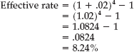
[78] "Using Cash Flow Information and Present Value in Accounting Measurements,"Statement of Financial Accounting Concepts No. 7 (Norwalk, Conn.: FASB, 2000).