Lesson 8
Properties of Least-squares Estimators

Summary

The purpose of this lesson is to apply results from Lessons 6 and 7 to least-squares estimators. First, small-sample properties are studied; then consistency is studied.

Generally, it is very difficult to establish small- or large-sample properties for least-squares estimators, except in the very special case when H(k) and V(k) are statistically independent. While this condition is satisfied in the application of identifying an impulse response, it is violated in the important application of identifying the coefficients in a finite-difference equation.

We also point out that many large-sample properties of LSEs are determined by establishing that the LSE is equivalent to another estimator for which it is known that the large-sample property holds true.

In Lesson 3 we noted that “Least-squares estimators require no assumptions about the nature of the generic model. Consequently, the formula for the LSE is easy to derive.” The price paid for not making assumptions about the nature of the generic linear model is great difficulty in establishing small- or large-sample properties of the resulting estimator.

When you complete this lesson you will be able to (1) explain the limitations of (weighted) least-squares estimators, so you will know when they can and cannot be reliably used, and (2) describe why you must be very careful when using (weighted) least-squares estimators.

Introduction

In this lesson we study some small- and large-sample properties of least-squares estimators. Recall that in least squares we estimate the n × 1 parameter vector θ of the linear model Z(k) = H(k)θ + V(k). We will see that most of the results in this lesson require H(k) to be deterministic or H(k) and V(k) to be statistically independent. In some applications one or the other of these requirements is met; however, there are many important applications where neither is met.

Small-Sample Properties of Least-Squares Estimators

In this section (parts of which are taken from Mendel, 1973, pp. 75-86) we examine the bias and variance of weighted least squares and least-squares estimators.

To begin, we recall Example 6-2, in which we showed that, when H(k) is deterministic, the WLSE of θ is unbiased. We also showed [after the statement of Theorem 6-2 and Equation (6-13)] that our recursive WLSE of θ has the requisite structure of an unbiased estimator, but that unbiasedness of the recursive WLSE of θ also requires h(k + 1) to be deterministic.

When H(k) is random, we have the following important result:

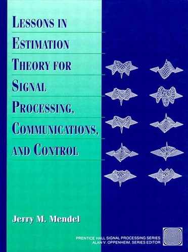
Theorem 8-1. The WLSE of θ,

(8-1)

is unbiased if V(k) is zero mean and if V(k) and H(k) are statistically independent.

Note that this is the first place (except for Example 6-2) where, in connection with least squares, we have had to assume any a priori knowledge about noise V(k).

Proof. From (8-1) and Z(k) = H(k)θ + V(k), we find that

(8-2)

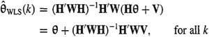
where, for notational simplification, we have omitted the functional dependences of H, W, and V on k. Taking the expectation on both sides of (8-2), it follows that

(8-3)

In deriving (8-3) we have used the fact that H(k) and V(k) are statistically independent [recall that if two random variables, a and b, are statistically independent p(a, b) = p(a)p(b); thus, E{ab} = E{a}E{b} and E{g(a)h(b)} = E{g(a)}E{h(b)}]. The second term in (8-3) is zero, because E{V} = 0, and therefore

(8-4)

This theorem only states sufficient conditions for unbiasedness of , which means that, if we do not satisfy these conditions, we cannot conclude anything about whether is unbiased or biased. To obtain necessary conditions for unbiasedness, assume that E{} = θ and take the expectation on both sides of (8-2). Doing this, we see that

(8-5)

E{(H′WH)^-1H′WV} = 0

Letting M = (H′WH)^-1H′W and m′_i denote the ith row of matrix M, (8-5) can be expressed as the following collection of orthogonality conditions:

(8-6)

Orthogonality [recall that two random variables a and b are orthogonal if E{ab} = 0] is a weaker condition than statistical independence, but is often more difficult to verify ahead of time than independence, especially since is a very nonlinear transformation of the random elements of H.

EXAMPLE 8-1

Recall the impulse response identification Example 2-1, in which θ = col[h(l), h(2),…, h(n)], where h(i) is the value of the sampled impulse response at time t_i. System input u(k) may be deterministic or random.

If {u(k), k = 0, 1,…, N – 1} is deterministic, then H(N – 1) [see Equation (2-5)] is deterministic, so that is an unbiased estimator of θ. Often, we use a random input sequence for {u(k), k = 0,1,…, N – 1}, such as from a random number generator. This random sequence is in no way related to the measurement noise process, which means that H(N – 1) and V(N) are statistically independent, and again will be an unbiased estimate of the impulse response coefficients. We conclude, therefore, that WLSEs of impulse response coefficients are unbiased.

EXAMPLE 8-2

As a further illustration of an application of Theorem 8-1, let us take a look at the weighted least-squares estimates of the n α-coefficients in the Example 2-2 AR model. We shall now demonstrate that H(N – 1) and V(N – 1), which are defined in Equation (2-8), are dependent, which means of course that we cannot apply Theorem 8-1 to study the unbiasedness of the WLSEs of the α-coefficients.

We represent the explicit dependences of H and V on their elements in the following manner:

(8-7)

H = H[y(N – 1), y(N – 2),…, y(0)]

and

(8-8)

V = V[u(N – 1), u(N – 2),…, u(0)]

Direct iteration of difference equation (2-7) for k = 1, 2,…, N – 1, reveals that y(1) depends on u(0),y(2) depends on u(1) and u(0), and finally that y(N – 1) depends on u(N – 2),…, u(0); thus,

(8-9)

H[y(N – 1), y(N – 2),…, y(0)] = H[u(N – 2), u(N – 3),…, u(0), y(0)]

Comparing (8-8) and (8-9), we see that H and V depend on similar values of random input u; hence, they are statistically dependent.

EXAMPLE 8-3

We are interested in estimating the parameter a in the following first-order system:

(8-10)

y(k+1) = –ay(k) + u(k)

where u(k) is a zero-mean white noise sequence. One approach to doing this is to collect y(k + 1), y(k),…, y(1) as follows:

(8-11)

and, to obtain . To study the bias of , we use (8-2) in which W(k) is set equal to I, and H(k) and V(k) are defined in (8-11). We also set = (k + 1). The argument of is k + 1 instead of k, because the argument of Z in (8-11) is k + 1. Doing this, we find that

(8-12)

Thus,

(8-13)

Note, from (8-10), that y(j) depends at most on u(j – 1); therefore,

(8-14)

because E{u(k)} = 0. Unfortunately, all the remaining terms in (8-13), i.e., for i = 0, 1,…,k – 1, will not be equal to zero; consequently,

(8-15)

E{(k + 1)} = a + 0 + k nonzero terms

Unless we are very lucky so that the k nonzero terms sum identically to zero, E{(k+l)} ≠α, which means, of course, that is biased.

The results in this example generalize to higher-order difference equations, so we can conclude that least-squares estimates of coefficients in an AR model are biased.

Next we proceed to compute the covariance matrix of , where

(8-16)

Theorem 8-2. If E{V(k)} = 0, V(K) and H(K) are statistically independent, and

(8-17)

E{V(k)V′(k)} = R(k)

then

(8-18)

Proof. Because E{V(K)} = 0 and V(k) and H(K) are statistically independent, E{} = 0, so

(8-19)

Using (8-2) in (8-16), we see that

(8-20)

Hence

(8-21)

where we have made use of the fact that W is a symmetric matrix and the transpose and inverse symbols may be permuted. From probability theory (e.g., Papoulis, 1991), recall that

(8-22)

Applying (8-22) to (8-21), we obtain (8-18).

Because (8-22) (or a variation of it) is used many times in this book, we provide a proof of it in the supplementary material at the end of this lesson.

As it stands, Theorem 8-2 is not too useful because it is virtually impossible to compute the expectation in (8-18), due to the highly nonlinear dependence of (H′WH)^-1H′WRWH(H′WH)^-1 on H. The following special case of Theorem 8-2 is important in practical applications in which H(K) is deterministic and R(k) = I. Note that in this case our generic model in (2-1) is often referred to as the classical linear regression model (Fomby et al., 1984), provided that

(8-23)

where Q is a finite and nonsingular matrix.

Corollary 8-1. Given the conditions in Theorem 8-2, and that H(K) is deterministic, and the components of V(k) are independent and identically distributed with zero-mean and constant variance , then

(8-24)

Proof. When H is deterministic, cov[] is obtained from (8-18) by deleting the expectation on its right-hand side. To obtain cov[] when cov [V(k)] = I, set W = I and R(k) = I in (8-18). The result is (8-24).

Theorem 8-3. If E{V(k)} = 0, H(k) is deterministic, and the components of V(k) are independent and identically distributed with constant variance , then is an efficient estimator within the class of linear estimators.

Proof. Our proof of efficiency does not compute the Fisher information matrix, because we have made no assumption about the probability density function of V(K).

Consider the following alternative linear estimator of θ:

(8-25)

where C(K) is a matrix of constants. Substituting (3-11) and (2-1) into (8-25), it is easy to show that

(8-26)

θ*(k) = (I + CH)θ + [(H′H)^-1 H′ + C]V

Because H is deterministic and E{V(K)} = 0,

(8-27)

E{θ*(k)} = (I + CH)θ

Hence, θ^*(k) is an unbiased estimator of θ if and only if CH = 0. We leave it to the reader to show that

(8-28)

Because CC′ is a positive semidefinite matrix, cov []≤ E{[θ*(k) – θ][θ*(k)–θ]′}; hence, we have now shown that satisfies Definition 6-3, which means that is an efficient estimator.

Usually, when we use a least-squares estimation algorithm, we do not know the numerical value of . If is known ahead of time, it can be used directly in the estimate of θ. We show how to do this in Lesson 9. Where do we obtain in order to compute (8-24)? We can estimate it!

Theorem 8-4. If E{V(k)} = 0, V(k) and H(k) are statistically independent [or H(k) is deterministic], and the components of V(k) are independent and identically distributed with zero mean and constant variance , then an unbiased estimator of is

(8-29)

where

(8-30)

Proof. We shall proceed by computing E{′(K)(K)} and then approximating it as ′(K)(k), because the latter quantity can be computed from Z(k) and , as in (8-30).

First, we compute an expression for (K). Substituting both the linear model for Z(k) and the least-squares formula for into (8-30), we find that

(8-31)

where I_k is the k × k identity matrix. Let

(8-32)

M = I_k – H(H′H)^-1H′

Matrix M is idempotent, i.e., M′ = M and M² = M; therefore,

(8-33)

Recall the following well-known facts about the trace of a matrix:

1. E{tr A} = trE{A}

2. trcA = ctrA, where c is a scalar

3. tr(A + B) = trA + trB

4. trI_N = N

5. tr AB = trBA

Using these facts, we now continue the development of (8-33) for the case when H(k) is deterministic [we leave the proof for the case when H(K) is random as an exercise], as follows:

(8-34)

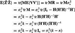
Solving this equation for , we find that

(8-35)

Although this is an exact result for , it is not one that can be evaluated, because we cannot compute E{′}

Using the structure of as a starting point, we estimate by the simple formula

(8-36)

To show that is an unbiased estimator of we observe that

(8-37)

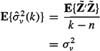
where we have used (8-34) for E{′}.

Large-Sample Properties of Least-Squares Estimators

Many large sample properties of LSEs are determined by establishing that the LSE is equivalent to another estimator for which it is known that the large-sample property holds true. In Lesson 11, for example, we will provide conditions under which the LSE of θ, , is the same as the maximum-likelihood estimator of θ, . Because is consistent, asymptotically efficient, and asymptotically Gaussian, inherits all these properties.

Theorem 8-5. If

(8-38)

exists, and

(8-39)

then

(8-40)

Assumption (8-38) postulates the existence of a probability limit for the second-order moments of the variables in H(k), as given by Σ_H. Note that H′(k)H(k)/k is the sample covariance matrix of the population covariance matrix Σ_H. Assumption (8-39) postulates a zero probability limit for the correlation between H(k) and V(k). H′(k)V(k) can be thought of as a “filtered” version of noise vector V(k). For (8-39) to be true, “filter H′(k)” must be stable. If, for example, H(k) is deterministic and , then (8-39) will be true. See Problem 8-10 for more details about (8-39).

Proof. Beginning with (8-2), but for instead of , we see that

(8-41)

Operating on both sides of this equation with plim and using properties (7-15), (7-16), and (7-17), we find that

which demonstrates that, under the given conditions, is a consistent estimator of θ.

In some important applications Eq. (8-39) does not apply, e.g., Example 8-2. Theorem 8-5 then does not apply, and the study of consistency is often quite complicated in these cases. The method of instrumental variables (Durbin, 1954; Kendall and Stuart, 1961; Young, 1984; Fomby et al., 1984) is a way out of this difficulty. For least squares the normal equations (3-13) are

(8-42)

In the method of instrumental variables, H′(k) is replaced by the instrumental variable matrix H′_IV(k) so that (8-42) becomes

(8-43)

Clearly,

(8-44)

In general, the instrumental variable matrix should be chosen so that it is uncorrelated with V(k) and is highly correlated with H(k). The former is needed so that is a consistent estimator of θ, whereas the latter is needed so that the asymptotic variance of does not become infinitely large (see Problem 8-12). In general, is not an asymptotically efficient estimator of θ (Fomby et al., 1984). The selection of H_IV(k) is problem dependent and is not unique. In some applications, lagged variables are used as the instrumental variables. See the references cited previously (especially, Young, 1984) for discussions on how to choose the instrumental variables.

Theorem 8-6. Let H_IV(k) be an instrumental variable matrix for H(k). Then the instrumental variable estimator , given by (8-44), is consistent.

Because the proof of this theorem is so similar to the proof of Theorem 8-5, we leave it as an exercise (Problem 8-11).

Theorem 8-7. If (8-38) and (8-39) are true, exists, and

(8-45)

then

(8-46)

where is given by (8-29).

Proof. From (8-31), we find that

(8-47)

Consequently,

Supplementary Material Expansion of Total Expectation

Here we provide a proof of the very important expansion of a total expectation given in (8-22), that

E_{H, v} {.} = E_H{E_V|H{. | H}}

Let G(H, V) denote an arbitrary matrix function of H and V [e.g., see (8-21)], and p(H, V) denote the joint probability density function of H and V. Then

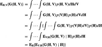
which is the desired result.

Summary Questions

1. When H(k) is random, is an unbiased estimator of θ:

(a) if and only if V(k) and H(k) are statistically independent

(b) V(k) is zero mean or V(k) and H(k) are statistically independent

(c) if V(k) and H(k) are statistically independent and V(k) is zero mean

2. If we fail the unbiasedness test given in Theorem 8-1, it means:

(a) must be biased

(b) could be biased

(c) is asymptotically biased

3. If H(k) is deterministic, then cov [] equals:

(a)(H′WH)^-1H′WRWH(H′WH)^-1

(b) H′WRWH

(c) (H′WH)^-2H′WRWH

4. The condition plim[H′(k)H(k)/k] = Σ_H means:

(a) H′(k)H(k) is stationary

(b) H′(k)H(k)/k converges in probability to the population covariance matrix Σ_H

(c) the sample covariance of H′(k)H(k) is defined

5. When H(k) can only be measured with errors, i.e., H_m(k) = H(k) +N(k), is:

(a) an unbiased estimator of θ

(b) a consistent estimator of θ

(c) not a consistent estimator of θ

6. When H(k) is a deterministic matrix, the WLSE of θ is:

(a) never an unbiased estimator of θ

(b) sometimes an unbiased estimator of θ

(c) always an unbiased estimator of θ

7. In the application of impulse response identification, WLSEs of impulse response coefficients are unbiased:

(a) only if the system’s input is deterministic

(b) only if the system’s input is random

(c) regardless of the nature of the system’s input

8. When we say that “ is efficient within the class of linear estimators,” this means that we have fixed the structure of the estimator to be a linear transformation of the data, and the resulting estimator:

(a) just misses the Cramer-Rao bound

(b) achieves the Cramer-Rao bound

(c) has the smallest error-covariance matrix of all such structures

9. In general, the instrumental variable matrix should be chosen so that it is:

(a) orthogonal to V(k) and highly correlated with H(k)

(b) uncorrelated with V(k) and highly correlated with H(k)

(c) mutually uncorrelated with V(k) and H(k)

Problems

8-1. Suppose that _LS is an unbiased estimator of θ. Is an unbiased estimator of θ²? (Hint: Use the least-squares batch algorithm to study this question.)

8-2. For to be an unbiased estimator of θ we required E{V(k)} = 0. This problem considers the case when E{V(k)} ≠ 0.

(a) Assume that E{V(k)} = V₀, where V₀ is known to us. How is the concatenated measurement equation Z(k) = H(k)θ + V(k) modified in this case so we can use the results derived in Lesson 3 to obtain or ?

(b) Assume that E{V(k)} = m_v1 where m_v is constant but is unknown. How is the concatenated measurement equation Z(k) = H(k)θ + V(k) modified in this case so that we can obtain least-squares estimates of both θ and m_v?

8-3. Consider the stable autoregressive model y(k) = θ₁y(k – 1)+…+θ_ky(k – K) +∈(k) in which the ∈(k) are identically distributed random variables with mean zero and finite variance σ². Prove that the least-squares estimates of θ₁,…,θ_k are consistent (see also, Ljung, 1976).

8-4. In this lesson we have assumed that the H(k) variables have been measured without error. Here we examine the situation when H_m(k) = H(k) + N(k) in which H(k) denotes a matrix of true values and N(k) a matrix of measurement errors. The basic linear model is now

Z(k) = H(k)θ + V(k) = H_m(k)θ +[V(k) – N(k)θ]

Prove that is not a consistent estimator of θ. See, also, Problem 8-15.

8-5. (Geogiang Yue and Sungook Kim, Fall 1991) Given a random sequence z(k) = a + bk + v(k), where v(k) is zero-mean Gaussian noise with variance , and E{v(i)v(j)} = 0 for all i≠ j. Show that the least-squares estimators of a and b, are unbiased.

8-6. (G. Caso, Fall 1991) [Stark and Woods (1986), Prob. 5.14] Let Z(N) = H(N)θ + V(N), where H(N) is deterministic, E{V(N)} = 0, and Φ = Dθ, where D is also deterministic.

(a) Show that for to be an unbiased estimator of Φ we require that LH(N) = D.

(b) Show that L = D[H′(N)H(N)]_-1H′(N) satisfies this requirement. How is related to for this choice of L?

8-7. (Keith M. Chugg, Fall 1991) This problem investigates the effects of preprocessing the observations. If is based on Y(k) = G(k)Z(k) instead of Z(k), where G(k) is an N × N invertible matrix:

(a) What is based on Y(k)?

(b) For H(k) deterministic and cov [V(k)] = R(k), determine the covariance matrix of .

(c) Show that for a specific choice of G(k),

What is the structure of the estimator for this choice of G(k)? (Hint: Any positive definite symmetric matrix has a Cholesky factorization.)

(d) What are the implications of part (c) and the fact that G(k) is invertible?

8-8. Regarding the proof of Theorem 8-3:

(a) Prove that θ^*(k) is an unbiased estimator of θ if and only if CH = 0.

(b) Derive Eq. (8-28).

8-9. Prove Theorem 8-4 when H(k) is random.

8-10. In this problem we examine the truth of (8-39) when H(k) is either deterministic or random.

(a) Show that (8-39) is satisfied when H(k) is deterministic, if

(b) Show that (8-39) is satisfied when H(k) is random if E{V(k)} = 0, V(k) and H k are statistically independent, and the components of V(k) are independent and identically distributed with zero mean and constant variance (Goldberger, 1964, pp. 269-270).

8-11. Prove Theorem 8-6.

8-12. (Fomby et al., 1984, pp. 258-259) Consider the scalar parameter model z(k) = h(k)θ + v(k), where h(k) and v(k) are correlated. Let h_iv(k) denote the instrumental variable for h(k). The instrumental variable estimator of θ is

Assume that v(k) is zero mean and has unity variance.

(a) Show that the asymptotic variance of is

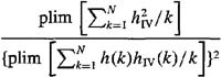
(b) Explain, based upon the result in part (a), why h_IV(k) must be correlated with h(k).

8-13. Suppose that ;, where Ω is symmetric and positive semidefinite. Prove that the estimator of given in (8-35) is inconsistent. Compare these results with those in Theorem 8-7. See, also, Problem 8-14.

8-14. Suppose that , where Ω is symmetric and positive semidefinite. Here we shall study (k), where [in Lesson 9 (k) will be shown to be a best linear unbiased estimator of θ, . Consequently, .

(a) What is the covariance matrix for ?

(b) Let , where . Prove that is an unbiased and consistent estimator of .

8-15. In this problem we consider the effects of additive noise in least squares on both the regressor and observation (Fomby et al, 1984, pp. 268-269). Suppose we have the case of a scalar parameter, such that y(k) = h(k)θ, but we only observe noisy versions of both y(k) and h(k), that is, z(k) = y(k) + v(k) and h_m(k) = h(k) + u(k). Noises v(k) and u(k) are zero mean, have variances and , respectively, and E{v(k)u(k)} = E{y(k)v(k)} = E{h(k)u(k)} = E{y(k)u(k)} = E{h(k)v(k)} = 0. In this case z(k) = h_m(k)θ+ ρ(k), where ρ(k) = v(k) – θu(k).

(a) Show that .

(b) Show that plim where .

Note that the method of instrumental variables is a way out of this situation.

8-16. This is a continuation of Problem 3-14, for restricted least squares.

(a) Show that is an unbiased estimator of θ.

(b) Let and . Prove that P^*(k)<P*(k).