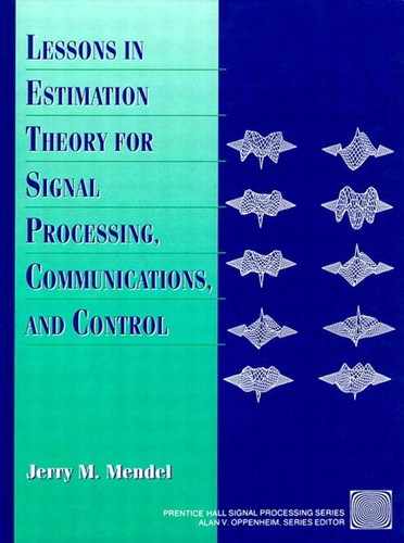
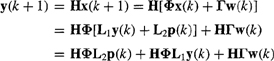
Lesson 22
State Estimation for the Not-so-basic State-variable Model

Summary

In deriving all our state estimators we worked with our basic state-variable model. In many practical applications we begin with a model that differs from the basic state-variable model. The purpose of this lesson is to explain how to use or modify our previous state estimators when there are:

1. Either nonzero-mean noise processes or known bias functions or both in the state or measurement equations; or

2. Correlated noise processes in the state and measurement equations; or

3. Colored disturbances or measurement noises; or

4. Some perfect measurements.

No new concepts are needed to handle items 1 and 2. A state augmentation procedure is needed to handle item 3. Colored noises are modeled as low-order Markov sequences, i.e., as low-order difference equations. The states associated with these colored noise models must be augmented to the original state-variable model prior to application of a recursive state estimator to the augmented system.

A set of perfect measurements reduces the number of states that have to be estimated. So, for example, if there are l perfect measurements, then we show how to estimate x(k) by a Kalman filter whose dimension is no greater than n – l. Such an estimator is called a reduced-order estimator of x(k). The payoff for using a reduced-order estimator is fewer computations and less storage.

In actual practice, some or all of the four special cases can occur simultaneously. Just merge the methods learned for treating each case separately to handle more complicated situations.

When you complete this lesson, you will be able to (1) use state estimation algorithms when the starting state-variable model differs from the basic state-variable model; and (2) apply state estimation to any linear, time-varying, discrete-time, nonstationary dynamical system.

Introduction

In deriving all our state estimators, we assumed that our dynamical system could be modeled as in Lessons 15, i.e., as our basic state-variable model. The results so obtained are applicable only for systems that satisfy all the conditions of that model: the noise processes w(k) and v(k) are both zero mean, white, and mutually uncorrelated, no known bias functions appear in the state or measurement equations, and no measurements are noise-free (i.e., perfect). The following cases frequently occur in practice:

1. Either nonzero-mean noise processes or known bias functions or both in the state or measurement equations

2. Correlated noise processes

3. Colored noise processes

4. Some perfect measurements

In this lesson we show how to modify some of our earlier results in order to treat these important special cases. To see the forest from the trees, we consider each of these four cases separately. In practice, some or all of them may occur together.

Biases

Here we assume that our basic state-variable model, given in (15-17) and (15-18), has been modified to

(22-1)

(22-2)

where W₁(k) and V₁(k) are nonzero mean, individually and mutually uncorrelated Gaussian noise sequences; i.e.,

(22-3)

(22-4)

E{[w₁(i)-m_w1(i)][w₁(j)-m_w1(j)]’} = Q(i)δ_ij,E{[v₁(i)-m_v1(i)][v₁(j)-m_v1(j)-m_v1(j)]’} = R(i)δ_ij, and E{[w₁(i)-m_w1(i)][v₁(j)-m_v1(j)]’} = 0. Note that the term G(k+1)u(k+1), which appears in the measurement equation (22-2), is known and can be thought of as contributing to the bias of V₁(k+1).

This case is handled by reducing (22-1) and (22-2) to our previous basic state-variable model, using the following simple transformations. Let

(22-5)

(22-6)

Observe that both w(k) and v(k) are zero-mean white noise processes, with covariances Q(k) and R(k), respectively. Adding and subtracting Γ(k + 1, k)m_w1(k) in state equation (22-1) and m_v1(k+1) in measurement equation (22-2), these equations can be expressed as

(22-7)

and

(22-8)

where

(22-9)

and

(22-10)

Clearly, (22-7) and (22-8) are once again a basic state-variable model, one in which u₁(k) plays the role of Ψ(k + 1, k)u(k) and z₁(k + 1) plays the role of z(k + 1).

Theorem 22-1. When biases are present in a state-variable model, then that model can always be reduced to a basic state-variable model [e.g., (22-7)to (22-10)]. All our previous state estimators can be applied to this basic state-variable model by replacing z(k) by z₁(k)and Ψ(k + 1, k)u(k) by u₁(k).

Correlated Noises

Here we assume that our basic state-variable model is given by (15-17) and (15-18), except that no w(k) and v(k) are correlated, i.e.,

(22-11)

There are many approaches for treating correlated process and measurement noises, some leading to a recursive predictor, some to a recursive filter, and others to a filter in predictor-corrector form, as in the following:

Theorem 22-2. When w(k) and v(k) are correlated, then a predictor-corrector form of the Kalman filter is

(22-12)

and

(22-13)

where Kalman gain matrix K(k+ 1) is given by (17-12), filtering-error covariance matrix P(k+ l|k+ 1) is given by (17-14), and predication-error covariance matrix P(k + 1 |k) is given by

(22-14)

in which

(22-15)

and

(22-16)

Observe that, if S(k) = 0, then (22-12) reduces to the more familiar predictor equation (16-4), and (22-14) reduces to the more familiar (17-13).

Proof. The derivation of correction equation (22-13) is exactly the same, when w(k) and v(k) are correlated, as it was when w(k) and v(k) were assumed uncorrelated. See the proof of part (a) of Theorem 17-1 for the details so as to convince yourself of the truth of this.

To derive predictor equation (22-12), we begin with the fundamental theorem of estimation theory; i.e.,

(22-17)

Substitute state equation (15-17) into (22-17) to show that

(22-18)

(22-19)

Let Z(k) = col (Z(k - 1), z(k)); then

In deriving (22-19) we used the facts that w(k) is zero mean, and w(k) and Z(k — 1) are statistically independent. Because w(k) and (k|k - 1) are jointly Gaussian,

(22-20)

Where is given by (16-33), and

(22-21)

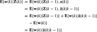
In deriving (22-21) we used the facts that and w(k) are statistically independent, and w(k) is zero mean. Substituting (22-21) and (16-33) into (22-20), we find that

(22-22)

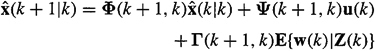
Substituting (22-22) into (22-19) and the resulting equation into (22-18) completes our derivation of the recursive predictor equation (22-12).

Equation (22-14) can be derived, along the lines of the derivation of (16-11), in a straightforward manner, although it is a bit tedious (Problem 22-1). A more interesting derivation of (22-14) is given in the Supplementary Material at the end of this lesson.

Recall that the recursive predictor plays the predominant role in smoothing; hence, we present the following corollary:

Corollary 22-1. When w(k) and v(k) are correlated, then a recursive predictor for x(k + 1) is

(22-23)

where

(22-24)

and

(22-25)

Proof. These results follow directly from Theorem 22-2; or they can be derived in an independent manner, as explained in Problem 22-1.

Corollary 22-2. When w(k) and v(k) are correlated, then a recursive filter for x(k+ 1) is

(22-26)

where

(22-27)

all other quantities have been defined above.

Proof. Again, these results follow directly from Theorem 22-2; however, they can also be derived, in a much more elegant and independent manner, as described in Problem 22-2.

Colored Noises

Quite often, some or all of the elements of either v(k) or w(k) or both are colored (i.e., have finite bandwidth). The following three-step procedure is used in these cases:

1. Model each colored noise by a low-order difference equation that is excited by white Gaussian noise.

2. Augment the states associated with the step 1 colored noise models to the original state-variable model.

3. Apply the recursive filter or predictor to the augmented system.

We try to model colored noise processes by low-order Markov sequences, i.e., low-order difference equations. Usually, first- or second-order models are quite adequate. Consider the following first-order model for colored noise process ω(k),

(22-28)

In this model n(k) is white noise with variance ; thus, this model contains two parameters, α and which must be determined from a priori knowledge about ω(k). We may know the amplitude spectrum of ω(k), correlation information about (ω(k), steady-state variance of ω(k), etc. Two independent pieces of information are needed in order to uniquely identify α and

EXAMPLE 22-1

We are given the facts that scalar noise w(k) is stationary with the properties E[w(k)} = 0 and E{w(i)w(j)} = e^–2|j–i|. A first-order Markov model for w(k) can easily be obtained as

(22-29)

(22-30)

EXAMPLE 22-2

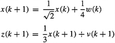
Here we illustrate the state augmentation procedure for the first-order system

(22-31)

(22-32)

where ω(k) is a first-order Markov sequence, i.e.,

(22-33)

and v(k) and n(k) are white noise processes. We augment (22-33) to (22-31), as follows. Let

(22-34)

Then (22-31) and (22-33) can be combined to give

(22-35)

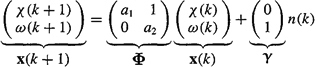
Equation (22-25) is our augmented state equation. Observe that it is once again excited by a white noise process, just as our basic state equation (15-17) is.

To complete the description of the augmented state-variable model, we must express measurement z(k + 1) in terms of the augmented state vector, x(k + 1); i.e.,

(22-36)

Equations (22-35) and (22-36) constitute the augmented state-variable model. We observe that, when the original process noise is colored and the measurement noise is white, the state augmentation procedure leads us once again to a basic (augmented) state-variable model, one that is of higher dimension than the original model because of the modeled colored process noise. Hence, in this case we can apply all our state estimation algorithms to the augmented state-variable model.

EXAMPLE 22-3

Here we consider the situation where the process noise is white but the measurement noise is colored, again for a first-order system:

(22-37)

(22-38)

As in the preceding example, we model v(k) by the following first-order Markov sequence

(22-39)

where n(k) is white noise. Augmenting (22-39) to (22-37) and reexpressing (22-38) in terms of the augmented state vector x(k), where

(22-40)

we obtain the augmented state-variable model

(22-41)

and

(22-42)

Observe that a vector process noise now excites the augmented state equation and that there is no measurement noise in the measurement equation. This second observation can lead to serious numerical problems in our state estimators, because it means that we must set R = 0 in those estimators, and, when we do this, covariance matrices become and remain singular.

Let us examine what happens to when covariance matrix R is set equal to zero. From (17-14) and (17-12) (in which we set R = 0), we find that

(22-43)

Multiplying both sides of (22-43) on the right by H'(k + 1), we find that

(22-44)

Because H'(k + 1) is a nonzero matrix, (22-44) implies that must be a singular matrix. We leave it to the reader to show that once becomes singular it remains singular for all other values of k.

EXAMPLE 22-4

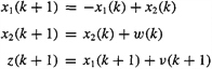
Consider the first-order system

(22-45)

(22-46)

where w(k) is white and Gaussian [ω(k) ~ N(ω(k);0, 1)] and v(k) is the noise process that is summarized in Figure 22-1, in which noise n(k) is also white and Gaussian )]. Our objective is to obtain a filtered estimate of x(k).

Figure 22-1 Noise model.

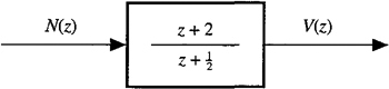
To begin, we shall demonstrate that passing white noise n(k) through the all-pass filter (z + 2)/(z + 1/2) once again leads to another white noise sequence, v(k). To show that v(k) is white we compute its power spectrum, using the fact that

(22-47)

in which

(22-48)

so that

(22-49)

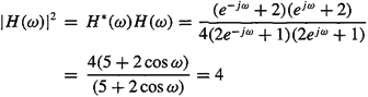
Consequently,

(22-50)

This shows that the power spectrum of v(k) is a constant; hence v(k) is a white process.

Next, we must obtain a state-variable model for the Figure 22-1 system. From an input/output point of view, the additive noise system is given by

(22-51)

Hence,

(22-52)

where

(22-53)

From this last equation, it follows that

(22-54)

Equations (22-54) and (22-52) are the state- variable model for the Figure 22-1 system.

To obtain a filtered estimate for state x(k), we must first combine the models in (22-45), (22-46), (22-54), and (22-52), by means of the state augmentation procedure. Letting , we obtain the following augmented state-variable model:

(22-55)

(22-56)

This state-variable model has correlated process and measurement noises, because n(k) appears in both noises; hence,

(22-57)

Using Theorem 22-2, we can compute and . To obtain the desired result, , just pick out the first element of , that is . We could also use Corollary 22-2 directly to obtain .

The key quantities that are needed to implement Theorem 22-2 are Φ₁ and Q₁, where

(22-58)

and

(22-59)

Perfect Measurements: Reduced-order Estimators

We have just seen that when R = 0 (or, in fact, even if some, but not all, measurements are perfect) numerical problems can occur in the Kalman filter. One way to circumvent these problems is ad hoc, and that is to use small values for the elements of covariance matrix R, even though measurements are thought to be perfect. Doing this has a stabilizing effect on the numerics of the Kalman filter.

A second way to circumvent these problems is to recognize that a set of “perfect” measurements reduces the number of states that have to be estimated. Suppose, for example, that there are l perfect measurements and that state vector x(k) is n × 1. Then, we conjecture that we ought to be able to estimate x(k) by a Kalman filter whose dimension is no greater than n – l. Such an estimator will be referred to as a reduced-order estimator. The payoff for using a reduced-order estimator is fewer computations and less storage.

To illustrate an approach to designing a reduced-order estimator, we limit our discussions in this section to the following time-invariant and stationary basic state-variable model in which and all measurements are perfect,

(22-60)

(22-61)

In this model y is l × 1. What makes the design of a reduced-order estimator challenging is the fact that the l perfect measurements are linearly related to the n states; i.e., H is rectangular.

To begin, we introduce a reduced-order state vector, p(k), whose dimension is (n – l) x 1; p(k) is assumed to be a linear transformation of x(k); i.e.,

(22-62)

Augmenting (22-62) to (22-61), we obtain

(22-63)

Design matrix C is chosen so that (H/C) is invertible. Of course, many different choices of C are possible; thus, this first step of our reduced-order estimator design procedure is nonunique. Let

(22-64)

where L₁ is n × l and L₂ is n × (n – l); thus,

(22-65)

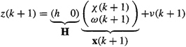
To obtain a filtered estimate of x(k), we operate on both sides of (22-65) with E{.|Y(k)}, where

(22-66)

Doing this, we find that

(22-67)

which is a reduced-order estimator for x(k). Of course, to evaluate , we must develop a reduced-order Kalman filter to estimate p(k). Knowing and y(k), it is then a simple matter to compute , using (22-67).

To obtain , using our previously derived Kalman filter algorithm, we first must establish a state-variable model for p(k). A state equation for p is easily obtained, as follows:

(22-68)

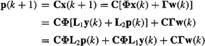
Observe that this state equation is driven by white noise w(k) and the known forcing function, y(k).

A measurement equation is obtained from (22-61) as

(22-69)

At time k + 1, we know y(k); hence, we can reexpress (22-69) as

(22-70)

where

(22-71)

Before proceeding any further, we make some important observations about our state-variable model in (22-68) and (22-70). First, the new measurement y₁(k + 1) represents a weighted difference between measurements y(k + 1) and y(k). The technique for obtaining our reduced-order state-variable model is, therefore, sometimes referred to as a measurement-differencing technique (e.g., Bryson and Johansen, 1965). Because we have already used y(k) to reduce the dimension of x(k) from n to n – 1, we cannot again use y(k) alone as the measurements in our reduced-order state-variable model. As we have just seen, we must use both y(k) and y(k + 1).

Second, measurement equation (22-70) appears to be a combination of signal and noise. Unless HΓ = 0, the term HΓw(k) will act as the measurement noise in our reduced-order state-variable model. Its covariance matrix is HΓQΓ'H'. Unfortunately, it is possible for HΓ to equal the zero matrix. From linear system theory, we known that HΓ is the matrix of first Markov parameters for our original system in (22-60) and (22-61), and HΓ may equal zero. If this occurs, we must repeat all the above until we obtain a reduced-order state vector whose measurement equation is excited by white noise. We see, therefore, that depending on system dynamics, it is possible to obtain a reduced-order estimator of x(k) that uses a reduced-order Kalman filter of dimension less than n – l.

Third, the noises that appear in state equation (22-68) and measurement equation (22-70) are the same, w(k); hence, the reduced-order state- variable model involves the correlated noise case that we described before in this chapter in the section entitled Correlated Noises.

Finally, and most important, measurement equation (22-70) is nonstandard, in that it expresses y₁ at k + 1 in terms of p at k rather than p at k + 1. Recall that the measurement equation in our basic state-variable model is z(k + 1) = Hx(k + 1) + v(k + 1). We cannot immediately apply our Kalman filter equations to (22-68) and (22-70) until we express (22-70) in the standard way.

To proceed, we let

(22-72)

so that

(22-73)

Measurement equation (22-73) is now in the standard from; however, because ζ(k) equals a future value of y₁, that is, y(k + 1), we must be very careful in applying our estimator formulas to our reduced-order model (22-68) and (22-73).

To see this more clearly, we define the following two data sets:

(22-74)

and

(22-75)

Obviously,

(22-76)

Letting

(22-77)

and

(22-78)

we see that

(22-79)

Equation (22-79) tells us to obtain a recursive filter for our reduced-order model; that is, in terms of data set D_y1(k + 1), we must first obtain a recursive predictor for that model, which is in terms of data set . Then, wherever ζ(k) appears in the recursive predictor, it can be replaced by y₁(k + 1).

Using Corollary 22-1, applied to the reduced-order model in (22-68) and (22-73), we find that

(22-80)

Thus,

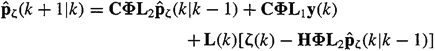
(22-81)

Equation (22-81) is our reduced-order Kalman filter. It provides filtered estimates of p(k + 1) and is only of dimension (n – l) × 1. Of course, when L(k) and P_y1 (k + l|k + l) are computed using (22-24) and (22-25), respectively, we must make the following substitutions:

Final Remark

To see the forest from the trees, we have considered each of our special cases separately. In actual practice, some or all of them may occur simultaneously. We have already seen one illustration of this in Example 22-4. As a guideline, you should handle the effects in your state-variable model in the order in which they were treated in this lesson. The exercises at the end of this lesson will permit you to gain experience with such cases.

Computation

Biases

Follow the procedure given in the text, which reduces a state-variable model that contains biases to our basic state-variable model. Then see the discussions in Lessons 17, 19, or 21 in order to do Kalman filtering or smoothing.

Correlated Noises

There is no M-file to do Kalman filtering for a time-varying or nonstationary state-variable model in which process and measurement noises are correlated. It is possible to modify our Kalman filter M-file, given in Lessons 17, to this case; and we leave this to the reader.

Using the Control System Toolbox, you must use two M-files. One (dlqew) provides gain, covariance, and eigenvalue information about the steady-state KF; the other (destim) computes both the steady-state predicted and filtered values for x(k).

dlqew: Discrete linear quadratic estimator design. Computes the steady-state Kalman gain matrix, predictor, and filter steady-state covariance matrices and closed-loop eigenvalues of the predictor. Does this for the following model (here we use the notation used in the Control System Toolbox reference manual):

where , and . The steady-state Kalman gain matrix, computed by dlqew, must be passed on to destim.

destim: Forms steady-state Kalman filter. Does this for the following model (here we use the notation used in the Control System Toolbox reference manual):

The state-variable model for the case of correlated noises can be put into the form of this model, by expressing it as

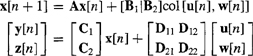
where y[n] are the sensor outputs and z[n] are the remaining plant outputs (if there are none, then set C₂ = D₂₁ = D₂₂ = 0). The partitioned matrices in this last system can then be equated to the plant matrices in the preceding basic state-variable model. Outputs steady-state predicted and filtered values for x(k), as well as the predicted value of the measurement vector y[n], all as functions of time.

Colored Noises

State augmentation is the workhorse for handling colored noises. It can be automatically accomplished for continuous-time systems (but not for discrete-time systems) by using the following M-file from the Control System Toolbox:

apend: Combines dynamics of two (continuous-time) state-space systems

Perfect Measurements

Here you must follow the text very closely. The state-variable model is given in Equations (22-68) and (22-73). It contains a known forcing function in the state equation and has correlated noises. See the subsection on Correlated Noises for how to proceed. Below Equation (22-79), it is stated that you need to obtain a recursive predictor for this model in order to compute the recursive filter for it.

Supplementary Material
Derivation of Equation (22-14)

The equation given in Theorem 22-2 for P(k + 1|k) has a very pleasant form; i.e., it looks just like the usual prediction error covariance equation, which is given in (16-11), except that Φ and Q have been replaced by Φ₁ and Q₁, respectively. Of course, (22-14) can be obtained by a brute-force derivation that makes extensive use of (22-12) and (22-13). Here we provide a more interesting derivation of (22-14), To begin, we need the following:

Theorem 22-3. The following identity is true:

(22-82)

Proof. From (22-13), we know that

(22-83)

Hence, (22-82) can be written as

or

or

Hence,

which reduces to the true statement that .

The importance of (22-82) is that it lets us reexpress the predictor, which is given in (22-12), as

(22-84)

where

(22-85)

Next, we show that there is a related state equation for which (22-84) is the natural predictor. The main ideas behind obtaining this related state equation are stated in Problem 22-2.

We begin by adding a convenient form of zero to state equation (15-17) in order to decorrelate the process noise in the modified basic state-variable model from the measurement noise v(k). We add D(k)[z(k) – H(k)x(k) – v(k)] to (15-17). The process noise, w₁(k), in the modified basic state-variable model, is equal to Γ(k + 1, k)w(k) – D(k)v(k). We choose the decorrelation matrix D(k) so that E{w₁(k)v′(k)} = 0, from which we find that

(22-86)

so that the modified basic state-variable model can be reexpressed as

(22-87)

Obviously, , given in (22-84), can be written by inspection of (22-87).

Return to Lesson 16 to see how P(k + l|k) was obtained. It is straightforward, upon comparison of (22-87) and (15-17), to show that

(22-88)

Finally, we need a formula for Q₁(k), the covariance matrix of W₁(k); but

(22-89)

and a simple calculation reveals that

(22-90)

This completes the derivation of (22-14).

Summary Questions

1. Mathematicians would describe the technique we have adopted for handling biases as:

(a) reductio ad absurdum

(b) reducing the problem to one for which we already have a solution

(c) induction

2. When colored noise is present in the state equation, the order of the final state-variable model:

(a) is always larger than the original order

(b) is sometimes larger than the original order

(c) can be smaller than the original order

3. When R(k) = 0:

(a) P(k + l|k) becomes singular for all k

(b) P(k + l|k + 1) becomes singular for all k

(c) K(k + 1) cannot be computed

4. If l perfect measurements are available, then we can estimate x(k) using a:

(a) unique reduced-order estimator

(b) nonunique KF

(c) nonunique reduced-order estimator

5. Suppose a system is described by a second-order state-variable model, one that is excited by a white disturbance noise w(k). Noisy measurements are made of y(k + 2). In this case:

(a) biases are present

(b) measurement noise is colored

(c) measurement noise and disturbance noise will be correlated

6. A reduced-order Kalman filter is one that:

(a) produces estimates of x(k)

(b) produces estimates of p(k)

(c) produces estimates of both x(k) and p(k)

7. The term state augmentation means:

(a) combine states in the original state-variable model

(b) switch to a new set of states

(c) append states to the original state vector

8. If l perfect measurements are available, then a reduced-order estimator:

(a) can be of dimension less than n–l

(b) must be of dimension n–l

(c) may be of dimension greater than n – l

Problems

22-1. Derive the recursive predictor, given in (22-23), by expressing as .

22-2. Here we derive the recursive filter, given in (22-26), by first adding a convenient form of zero to state equation (15-17), in order to decorrelate the process noise in this modified basic state- variable model from the measurement noise v(k). Add D(k)[z(k) – H(k)x(k) – v(k)] to (15-17). The process noise, W₁(k), in the modified basic state-variable model, is equal to Γ(k + 1, k)w(k)– D(k)v(k). Choose “decorrelation” matrix D(k) so that E{w₁(k)v′(k)} = 0. Then complete the derivation of (22-26).

22-3. In solving Problem 22-2 we arrive at the following predictor equation:

Beginning with this predictor equation and corrector equation (22-13), derive the recursive predictor given in (22-23).

22-4.Show that once becomes singular it remains singular for all other values of k.

22-5. Assume that R = 0, HΓ = 0, and HΦΓ 0. Obtain the reduced-order estimator and its associated reduced-order Kalman filter for this situation. Contrast this situation with the case given in the text, for which HΓ 0.

22-6. Develop a reduced-order estimator and its associated reduced-order Kalman filter for the case when l measurements are perfect and m – l measurements are noisy.

22-7. (Tom F. Brozenac, Spring 1992) (a) Develop the single-stage smoother in the correlated noise case, (b) Develop the double-stage smoother in the correlated noise case, (c) Develop formulas for in the correlated noise case, (d) Refer to Example 21-1, but now w(k) and v(k) are correlated, and E{w(i)v(j) } = 0.5δ(i, j). Compute the analogous quantities of Table 21-1 when N = 4.

22-8. Consider the first-order system and z(k + 1) = x(k + 1) + v(k + 1), where E{w₁(k)} = 3, E{v(k)} = 0, w₁(k) and v(k) are both white and Gaussian, E{w²₁ (k)} = 10, E{v² k} = 2, and w₁(k) and v(k) are correlated; i.e., E{w₁ (k)v(k)} = 1.

(a) Obtain the steady-state recursive Kalman filter for this system.

(b) What is the steady-state filter error variance, and how does it compare with the steady-state predictor error variance?

22-9. Consider the first-order system and z(k + 1) = x(k + 1) + v(k + 1), where w(k) is a first-order Markov process and v(k) is Gaussian white noise with E{v(k)} = 4, and r = 1.

(a) Let the model for w(k) be w(k + 1) = αw(k) + u(k), where u(k) is a zeromean white Gaussian noise sequence for which E{u²(k)} = Additionally, E{w(k)} = 0. What value must a have if E{w²(k)} = W for all k?

(b) Suppose W² = 2 and = 1. What are the Kalman filter equations for estimation of x(k) and w(k)?

22-10. Obtain the equations from which we can find , , and for the following system:

where v(k) is a colored noise process; i.e.,

Assume that w(k) and n(k) are white processes and are mutually uncorrelated, and = 2. and = 2. Include a block diagram of the interconnected system and reduced-order KF.

22-11. Consider the system x(k + 1) = Φx(k) + γµ(k) and , where µ(k) is a colored noise sequence and v(k) is zero-mean white noise. What are the formulas for computing ? Filter is a deconvolution filter.

22-12. Consider the scalar moving average (MA) time-series model

z(k) = r(k)+r(k-1)

where r(k) is a unit variance, white Gaussian sequence. Show that the optimal one-step predictor for this model is [assume = 1]

(Hint: Express the MA model in state-space form.)

22-13. Consider the basic state-variable model for the stationary time-invariant case. Assume also that w(k) and v(k) are correlated; i.e.,

(a) Show, from first principles, that the single-stage smoother of x(k), i.e.,, is given by

where is an appropriate smoother gain matrix.

(b) Derive a closed-form solution for as a function of the correlation matrix S and other quantities of the basic state-variable model.

22-14. (Tony Hung-yao Wu, Spring 1992) In the section entitled Colored Noises we modeled colored noise processes by low-order Markov processes. We considered, by means of examples, the two cases when either the disturbance is colored, but the measurement noise is not, or the measurement noise is colored, but the disturbance is not. In this example, consider the case when both the disturbance and the measurement noises are colored, when the system is first-order. Obtain the augmented SVM for this situation, and comment on whether or not any difficulties occur when using this SVM as the starting point to estimate the system’s states using a KF.

22-15. Given the state-variable model where now w(k) = col (w₁(k), w₂(k) in which W₁(k) is white with covariance matrix Q₁(k), but is nonzero mean, and w₂(k) is colored and is modeled as a vector first-order Markov sequence. Reformulate this not-so-basic state-variable model so that you can estimate x(k) by a Kalman filter designed for the basic SVM.

22-16. (Tony Hung-yao Wu, Spring 1992) Sometimes noise processes are more accurately modeled as second-order Markov sequences rather than as first-order sequences. Suppose both w(k) and v(k) are described by the following second-order sequences:

w(k + 2) = b₁w(k+l) + b₂ w(k)+ n_w(k)

v(k + 2) = C_l v(k + 1) + c₂ v(K) + n_v (k)

The system is the first-order system given in (22-31) and (22-32). Obtain the augmented SVM for this situation, and comment on whether or not any difficulties occur when using it as the starting point to estimate the system’s states using a KF.

22-17. Consider the following first-order basic state-variable model:

where

(a) What is the steady-state value of the variance of z(k + 1)?

(b) What is the structure of the Kalman filter in predictor-corrector format?

(c) It is claimed that the Kalman gain is the same as in part (c) of Problem 19-12, because Theorem 22-2 states “Kalman gain matrix, K(k + 1), is given by (17-12)….” Explain whether this claim is true or false.

22-18. Given the following second-order SVM:

where . Obtain a first-order KF for expressed in predictor-corrector format. Include all equations necessary to implement this filter using numerical values from the given model.