Lesson C
Estimation and Applications of Higher-order Statistics
Summary
Higher-order statistics can either be estimated from data or computed from models. In this lesson we learn how to do both. Cumulants are estimated from data by sample-averaging techniques. Polyspectra are estimated from data either by taking multidimensional discrete-time Fourier transforms of estimated cumulants or by combining the multidimensional discrete Fourier transform of the data using windowing techniques. Because cumulant and polyspectra estimates are random, their statistical properties are important. These properties are described.
Just as it is important to be able to compute the second-order statistics of the output of a single-input, single-output dynamical system, it is important to be able to compute the higher-order statistics of the output for such a system. This can be accomplished using the Bartlett-Brillinger-Rosenblatt formulas. One formula lets us compute the Mi-order cumulant of the system’s output from knowledge about the system’s impulse response. Another formula lets us compute the fob-order polyspectrum of the system’s output from knowledge about the Fourier transform of the system’s impulse response.
Not only are the Bartlett-Brillinger-Rosenblatt formulas useful for computing cumulants and polyspectra for given systems, but they are also the starting points for many important related results, including a closed-form formula (the C(q, k) formula) for determining the impulse response of an MA(q) system; a closed-form formula (the g-slice formula) for determining the impulse response of an ARMA(p, q) system, given that we know the AR coefficients of the system; cumulant-based normal equations for determining the AR coefficients of either an AR (p) system or an ARMA (p, q) system; a nonlinear system of equations (the GM equations) that relates second-order statistics to higher-order statistics, which can be used to determine the coefficients of an MA(q) system; and equations that relate a system and its inverse, which lead to new optimal deconvolution filters that are based on higher-order statistics.
When you complete this lesson, you will be able to (1) estimate cumulants from data; (2) estimate polyspectra from data; (3) understand the statistical properties of cumulant and polyspectral estimators; (4) derive the Bartlett-Brillinger Rosenblatt formulas; (4) apply the Bartlett-Brillinger-Rosenblatt formulas to compute cumulants and polyspectra for single-input and single-output dynamical systems; and (5) understand many applications of the Bartlett-Brillinger-Rosenblatt formulas to system identification and deconvolution problems.
Estimation of Cumulants (Nikias and Mendel, 1993)
In many practical situations we are given data and want to estimate cumulants from the data. Later in this lesson we describe applications where this must be done in order to extract useful information about non-Gaussian signals from the data. Cumulants involve expectations and cannot be computed in an exact manner from real data; they must be estimated, in much the same way that correlations are estimated from real data. Cumulants are estimated by replacing expectations by sample averages; i.e.,
(c-1)
![]()
where NR is the number of samples in region R. A similar but more complicated equation can be obtained for ![]() by beginning with (B-12c) (Problem C-l). It will not only involve a sum of a product of four terms [analogous to (c-1)] but it will also involve products of sample correlations, where
by beginning with (B-12c) (Problem C-l). It will not only involve a sum of a product of four terms [analogous to (c-1)] but it will also involve products of sample correlations, where
(c-2)

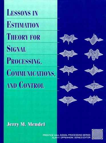
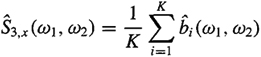
A practical algorithm for estimating C3, x(τ1,τ2) is (Nikias and Mendel, 1993): Let {x(l),x(2),…,x(N)} be the given data set; then (1) segment the data into K records of M samples each, i.e., N = K M; (2) subtract the average value of each record; (3) assuming that {x(i)(k),k = 0, 1,…,M-1}, is the zero-mean data set per segment i = 1,2,…, k, obtain an estimate of the thirdmoment sequence
(c-3)
where i = 1,2,…, K;S1 = max(0,-τ1,-τ2); and, s2 = min(M -1, M - 1-τ1, M -1- τ2) (Problem C-2); (4) average ![]() (τ1τ2 over all segments to obtain the final estimate
(τ1τ2 over all segments to obtain the final estimate
(C-4)

Of course, we should use the many symmetry properties of third (fourth)-order cumulants, which are given in Lesson B, to reduce the number of computations.
It is well known (e.g., Ljung and Soderstrom, 1983, and Priestley, 1981) that exponential stability of the underlying channel model guarantees the convergence in probability of the sampled autocorrelation function to the true autocorrelation function. A correlation estimator that uses several independent realizations is very reliable, since doing this reduces the variance of the estimator. It is preferrable to use a biased unsegmented correlation estimator to an unbiased unsegmented correlation estimator, because the biased estimator leads to a positive-definite covariance matrix, whereas the unbiased estimator does not (Priestley, 1981). When we only have a single realization, as is often the case in signal-processing applications, the biased segmented estimator gives poorer correlation estimates than both the unbiased segmented estimator and the biased unsegmented estimator. Some of these issues are explored in Problems C-3 and C-4 at the end of this lesson.
The convergence of sampled third-order cumulants to true third-order cumulants is studied in Rosenblatt and Van Ness (1965). Essentially, if the underlying channel model is exponentally stable, input random process v(ri) is stationary, and its first six (eight) cumulants are absolutely summable, then the sampled third-order (fourth-order) cumulants converge in probability to the true third-order (fourth-order) cumulants. Additionally, sampled third-order and fourth-order cumulants are asymptotically Gaussian (Giannakis and Swami, 1990; Lii and Rosenblatt, 1982,1990; and Van Ness, 1966). Consequently, we are able to begin with an equation like
(c-5)
![]()
in which estimation error is asymptotically Gaussian and to ex classification or detection procedures to this formulation.
Formulas for estimating the covariances of higher-order moment estimates can be found in Friedlander and Porat (1990) and Porat and Friedlander (1989). Although they are quite complicated, they may be of value in certain methods where estimates of such quantities are needed.
The reason it is important to know that sample estimates of cumulants converge in probability to their true values (i.e., are consistent) is that functions of these estimates are used in many of the techniques that have been developed to solve a wide range of signal-processing problems. From Lessons 7, we know that arbitrary functions of consistent estimates are also consistent; hence, we are assured of convergence in probability (or sometimes with probability 1) when using these techniques.
From Lessons 11, we know that sampled estimates of Gaussian processes are also optimal in a maximum-likelihood sense; hence, they inherit all the properties of such estimates. Unfortunately, sampled estimates of non-Gaussian processes are not necessarily optimal in any sense; hence, it may be true that estimates other than the conventional sampled estimates provide “better” results.
Estimation of Bispectrum (Nikias and Mendel, 1993)
There are two popular approaches for estimating the bispectrum, the indirect method and the direct method, both of which can be viewed as approximations of the definition of the bispectrum. Although these approximations are straightforward, sometimes the required computations may be expensive despite the use of fast Fourier transform (FFT) algorithms. We will briefly describe both conventional methods. Their extensions to trispectrum estimation is described in Nikias and Petropulu(1993).
Indirect Method
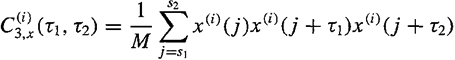
Let {x(1), x(2),…, x(N)}, be the given data set; then (1) estimate cumulants using segmentation and averaging, as described in the preceding section, to obtain ![]() in (C-4); and (2) generate the bispectrum estimate
in (C-4); and (2) generate the bispectrum estimate
(c-6)
where L < M – 1 and W(τ1,τ2) is a two-dimensional window function. For discussions on how to choose the window function, see Nikias and Petropulu (1993). ![]()
This method is “indirect” because we first estimate cumulants, after which we take their two-dimensional discrete-time Fourier transforms (DTFT). Of course, the computations of the bispectrum estimate may be substantially reduced if the symmetry properties of third-order cumulants are taken into account for the calculations of ![]() and if the symmetry properties of the bispectrum, as discussed in Lesson B, are also taken into account.
and if the symmetry properties of the bispectrum, as discussed in Lesson B, are also taken into account.
Direct Method
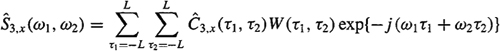
Let {x(l),x(2),…, x(N)}be the given data set. Assume that fs is the sampling frequency and Δ0 = fs/N0 is the required spacing between frequency samples in the bispectrum domain along horizontal or vertical directions; thus, N0 is the total number of frequency samples. Then (1) segment the data into K segments of M samples each, i.e., N = KM, and subtract the average value of each segment. If necessary, add zeros at the end of each segment to obtain a convenient (even) length M for the FFT; (2) assuming that {x(i) (k), k = 0, 1,…, M–1}, is the data set per segment i = 1,2,…, K, generate the discrete Fourier transform (DFT) coefficients (Brigham, 1988) Y(i)(λ),i = l,2,…,K, where
(c-7)
and λ= 0, 1,…, M/2; (3) form the bispectrum estimate [motivated by (C-17) for k = 3] based on the DFT coefficients
(c-8)
![]()
over the triangular region 0 ≤ λ2≤ λ1,λ1+λ2=Fs/2. In general, M = M1×N0, where M1 is a positive integer (assumed odd); i.e., M1 = 2L1 + 1. Since M is even and M1 is odd, we compromise on the value of N0 (closest integer). In the special case where no averaging is performed in the bispectrum domain, M1 = 1 and L1= 0, in which case
(c-9)
![]()
(4) the bispectrum estimate of the given data is the average over the K segments;i.e.,
(c-10)
where
(c-11)
![]()
This method is called “direct” because all calculations are in the frequency domain.
The statistical properties of the direct and indirect conventional methods for bispectrum estimation have been studied by Rosenblatt and Van Ness (1965), Van Ness (1966), Brillinger and Rosenblatt (1967a), and Rao and Gabr (1984). Their implications in signal processing have been studied by Nikias and Petropulu (1993). The key results are that both methods are asymptotically unbiased, consistent, and asymptotically complex Gaussian. Formulas for their asymptotic variances can be found in Nikias and Petropulu (1993, p. 143). From these formulas, we can conclude that the variance of these conventional estimators can be reduced by (1) increasing the number of records (K), (2) reducing the size of support of the window in the cumulant domain (L) or increasing the size of the frequency smoothing window (Mi), and (3) increasing the record size (M). Increasing the number of records (K) is demanding on computer time and may introduce potential nonstationarities. Frequency-domain averaging over large rectangles of size M1 or use of cumulant-domain windows with small values of LQ reduces frequency resolution and may increase bias. In the case of “short length” data, K could be increased by using overlapping records (Nikias and Raghuveer, 1987).
Both conventional methods have the advantage of ease of implementation (FFT algorithms can be used) and provide good estimates for sufficiently long data; however, because of the “uncertainty principle” of the Fourier transform, the ability of the conventional methods to resolve harmonic components in the bispectral domain is limited.
Applications of Higher-order Statistics to Linear Systems
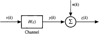
A familiar starting point (some of the material in this section is taken from Mendel,1991) for many problems in signal-processing and system theory is the single-input, single-output (SISO) linear and time-invariant (LTI) model depicted in Figure C-1, in which v(k) is white Gaussian noise with finite variance ![]() ,H(z)[h(k)] is causal and stable, n(k) is also white Gaussian noise with variance
,H(z)[h(k)] is causal and stable, n(k) is also white Gaussian noise with variance ![]() , and v(k) and n(k) are statistically independent. Letting r(.) and S(.) denote correlation and power spectrum, respectively, then it is well known (Problem C-5) that (e.g., Papoulis, 1991)
, and v(k) and n(k) are statistically independent. Letting r(.) and S(.) denote correlation and power spectrum, respectively, then it is well known (Problem C-5) that (e.g., Papoulis, 1991)
(c-12)
![]()
(c-13)
![]()
and
(c-14)
![]()
From (C-13) we see that all phase information has been lost in the spectrum (or in the autocorrelation); hence, we say that correlation or spectra are phase blind.
Bartlett(1955) and Brillinger and Rosenblatt (1967b) established a major generalization to Equations (C-12) and (C-13). In their case the system in Figure C-l is assumed to be causal and exponentially stable, and (v(k)} is assumed to be independent, identically distributed (i.i.d.), and non-Gaussian; i.e.,
(c-15)
![]()
where γk, v denotes the kth-order cumulant of v(i). Additive noise n(k) is assumed to be Gaussian, but need not be white.
Theorem C-l.
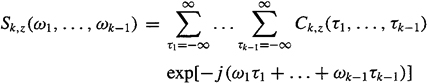
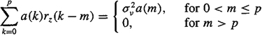
For the single-channel system depicted in Figure C-l, if{v(i)} is independent, identically distributed (i.i.d.), and non-Gaussian, as in (C-l5), and n(k) is Gaussian (colored or white), then the kth-order cumulant and poly spectra of measured signal z(k) are
Figure C-l Single-channel system
(c-16)
![]()
(c-17)
![]()
where k > 3.
This theorem generalizes our statistical characterization and understanding of the system in Figure C-l, from second- to higher-order statistics. It is even valid for k = 2 by replacing z(k) by y(k). In that case, (C-l6) and (C-l7) reduce to C2, y(τ1)=γ2, vΣh(n)h(n+τ1) and ![]() Note that (C-l2) and (C-l3) are the correct second-order statistics for noisy measurement z(k). Equations (C-16) and (C-17) have been the starting points for many nonparametric and parametric higher-order statistics techniques that have been developed during the past 10 years [e.g., Nikias and Raghuveer (1987) and Mendel(1988)].
Note that (C-l2) and (C-l3) are the correct second-order statistics for noisy measurement z(k). Equations (C-16) and (C-17) have been the starting points for many nonparametric and parametric higher-order statistics techniques that have been developed during the past 10 years [e.g., Nikias and Raghuveer (1987) and Mendel(1988)].
Proof. (Mendel, 1991) Because n(k) is assumed to be Gaussian, the Mil- order cumulant of z(k) equals the fob-order cumulant of y(k), where
(c-18)

Note that the following derivation is expedited by working with the more general form in (C-18), where i ranges from –∞ to ∞, instead of the form associated with a causal IR for which i ranges from 0 to k. Changes of variables then do not change the ranges of the summation. Consequently,
(c-19)
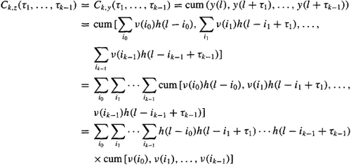
To arrive at the third line of this derivation, we have used cumulant property [CP3];and to arrive at the fourth line, we have used cumulant property [CP1] (see Lesson B).
In the case of a white noise input, (C-l9) simplifies considerably to 
which is (C-16). To arrive at the first line, we have used (C-15), noting that
(c-20)
And to arrive at the second line of (C-19), we have made a simple substitution of variables and invoked the stationarity of y(n) and the causality of h(n). The former tells us that Ck, y(τ1,…,τk-1) = Ck, z(τ1,…, τk-1) will not depend on time n; the latter tells us that h(ri) = 0 for n < 0.
The polyspectrum in (C-17) is easily obtained by taking the (k – 1)-dimensional discrete-time Fourier transform of (C-16):
(c-21)
Substitute (C-16) into (C-21) to obtain (C-17) (problem C-6).![]()
From this proof, we observe that (C-16) and (C-17) are also valid for noncausal systems, in which case N ranges from – ∞ to∞ in (C-16).
The generalization of (C-16) to the case of a colored non-Gaussian input v(i) is [Bartlett (1955) only considers the k = 2,3,4 cases; Brillinger and Rosenblatt(1967b) provide results for all k]
(c-22
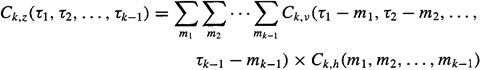
where
(c-23)
![]()
A derivation of this result is requested in Problem C-7. Observe that the right-hand side of (C-22) is a multidimensional convolution of Ck, v(τ1,…,τk-1) with the deterministic correlation function of h(n), which we have denoted Ck, h(m1,m2,…,Mk-1). Consequently, the generalization of (C-17) to the case of a colored non-Gaussian input v(i) is
(c-24)
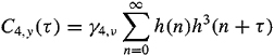
One very important use for (C-16) is to compute cumulants for models of systems. The procedure for doing this is (1) determine the model’s IR, h(k), k = 0, 1, 2,…, K; (2) fix the τj values at integers, and evaluate (C-16); and (3) repeat step 2 for all τj values in the domain of support of interest (be sure to use the symmetry properties of cumulants to reduce computations). This is how the results in Figures B-3(c) and (d), (B-4), and (B-5) were obtained.
Similarily, a very important use of (C-17) is to compute polyspectra for models. The procedure for doing this is (1) determine the model’s IR, h(k), k = 0, 1, 2,…, K; (2) compute the DTFT of h(k), H(ω); (3) fix the ωj values and evaluate (C-17); and (4) repeat step 3 for all ωj values in the domain of support of interest (be sure to use the symmetry properties of polyspectra to reduce computations). This is how the results in Figures B-7 were obtained. Of course, another way to compute the polyspectra is to first compute the cumulants, as just described, and then compute their multidimensional DTFT’s.
EXAMPLE C-l MA(q) Model (Mendel, 1991)
Suppose that h(k) is the impulse response of a causal moving average (MA) system. Such a system has a finite IR and is described by the following model:
(C-25)
![]()
The MA parameters are b(0), b(l),…,b(q), where q is the order of the MA model and b(0) is usually assumed equal to unity [the scaling is absorbed into the statistics of v(k)]. It is well known that for this model h(i) = b(i), i = 0,1,…, q; hence, when {v(l)} is i.i.d., we find from (C-16) that
(C-26)
![]()
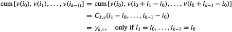
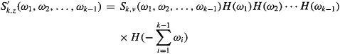
An interesting question is, “For which values of τ1 and τ2 is C3, y(τ1, τ2) nonzero?” The answer to this question is depicted in Figure C-2. The domain of support for C3, y(τ1 = m, τ2 = n) is the six-sided region. This is due to the FIR nature of the MA system. The triangular region in the first quadrant is the principal region. In the stationary case, we only have to determine third-order cumulant values in this region, R, where
(C-27)
![]()
Observe, from Figure C-2, that the third-order cumulant equals zero for either one or both of its arguments equal to q + 1. This suggests that it should be possible to determine the order of the MA model, q, by testing, in a statistical sense, the smallness of a third-order cumulant such as C3, y(q + 1, 0). See Giannakis and Mendel (1990) for how to do this.![]()
EXAMPLE C-2 C(q, k) Formula
Equation (C-14) is a “classical” way for computing the impulse response of a SISO system; however, it requires that we have access to both the system’s input and output in order to be able to compute the cross-correlation rvz(k). In many applications, we have access only to a noise-corrupted version of the system’s output (e.g., blind equalization, reflection seismology). A natural question to ask is, “Can the system’s IR be determined just from output measurements?” Using output cumulants, the answer to this question is yes. Giannakis (1987b) was the first to show that the IR of a qth-order MA system can be calculated just from the system’s output cumulants.
Figure C-2 The domain of support for C3, y(τ1,τ2) for an MA(q) system. The horizontally shaded triangular region is the principal region.
We begin with (C-16) for k = 3; i.e.,
(C-28)
![]()
in which h(0) = 1, for normalization purposes. Set τ1 = q and τ2 = k in (C-28), and use the fact that for an MA(q) system h(j) = 0∀j > q, to see that
(C-29)
![]()
Next, set τ1 = q and τ2 = 0 in (C-28) to see that
(C-30)
![]()
Dividing (C-29) by (C-30), we obtain the “C(q, k) formula,”
(C-31)
![]()
This is a rather remarkable theoretical result in that it lets us determine a system’s IR just from system output measurements. Observe that it only uses values of third-order cumulants along the right-hand side of the principal region of support (seeFigure C-2).
The C(q, k) formula can be generalized to arbitrary-order cumulants (Problem C-8), and, as a byproduct, we can also obtain formulas to compute the cumulant of the white input noise (Problem C-9).![]()
Corollary C-l. Suppose that h(k) is associated with the following ARMA (p, q) model
(C-32)

(C-33)
![]()
This rather strange looking result (Swarni and Mendel, 1990b) has some very nteresting applications, as we shall demonstrate later.
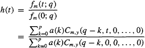
Proof. To begin, we define the scalar function ƒm(t; τ) as
(C-34)
![]()
If we know both the AR coefficients and the output cumulants, then we can compute ƒm(t; τ) for different values of t and τ. Next, substitute (C-16) into the right-hand side of (C-34) to see that
(C-35)
![]()
Impulse response h(n) of the ARMA (p, q) model in (C-32) satisfies the recursion
(C-36)
![]()
Hence, we recognize that the sum on the far right of (C-35) equals b(i + τ), so (C-35) becomes
(C-37)
![]()
Finally, to obtain the right-hand side of (C-33) from (C-37); let i + τ = j; truncate the upper limit in the summation from ∞ to q, because b(j) = 0 ∀j > q; and extend the lower limit in the summation from j = τ to j = 0, because h(l) is causal [so that h(–τ) = h(–τ + l)=… = h(–l) = 0].![]()
EXAMPLE C-3 q-Slice Formula
From (C-37) and the fact that b(j) = 0 for ∀ j > q, it is straightforward to show that
(C-38)
![]()
and
(C-39)
![]()
Consequently,
(C-40)
where t = 0,1,…. This is a closed-form formula for the IR of an ARMA(p, q) system (Swami and Mendel, 1990b). When p = 0, then (C-40) reduces to the C(q,K) formula. To use (C-40), the AR parameters must be known, and we must estimate the cumulants in its numerator and denominator.
It is easy to show that (C-36) can be used to compute the MA coefficients b(1), b(2),…, b(q) if we are given all the AR coefficients and IR values h(0), h(l),…, h(q) (Problem C-10). Because of normalization, h(0) = 1; hence, we can use (C-40) to compute h(l),…, h(q). For each value of t, the numerator cumulants must be estimated along a horizontal slice, ranging from τ1 = q – p (which will be negative, because p > q) to τ1 = q. The denominator of (C-40) only needs to be computed one time, and it uses cumulants along a horizontal slice along the τ1 axis, where again T1 ranges from τ1 = q – p to τ1 = q. Because the numerator slice changes with each calculation of h(t), and we need to compute q values of h(t), (C-40) is known as the q-slice algorithm (Swami and Mendel, 1990b). The q-slice algorithm can be used as part of a procedure to estimate the coefficients in an ARMA(p, q) system (Problem C-21).![]()
EXAMPLE C-4 Cumulant-based Normal Equations
Many ways exist for determining the AR coefficients of either the ARMA (p, q) model in (C-32) or the following AR(p) model:
(C-41)
![]()
where a(0) = 1. One of the most popular ways is to use the following correlation-based normal equations (Box and Jenkins, 1970) (Problem C-ll):
(C-42)
![]()
If AR order p is known, then (C-42) is collected for p values of m, from which the AR coefficients a(l), a(2),…, a(p) can be determined. Note that (C-42) is also true for an ARMA(p, q) model when m > q. The correlation-based normal equations do not lead to very good results when only a noise-corrupted version of y(k) is available, because additive Gaussian measurement noise seriously degrades the estimation of ry (k – m); hence, we are motivated to seek alternatives that are able to suppress additive Gaussian noise. Cumulants are such an alternative.
Starting with (C-33), it follows that
(C-43)
![]()
From the causality of h(l), it follows that the right-hand side of (C-43) is zero for τ > q; hence,
(C-44)
![]()
Of course, in the AR case q = 0, so in this case the right-hand side of (C-44) is zero for τ >0.
Equation (C-44) is a cumulant-based normal equation and should be compared with (C-42). Parzen (1967) credits Akaike (1966) for the “idea of extending” correlation-based normal equations to cumulants. See, also, Giannakis (1987a), Giannakis and Mendel (1989), Swami (1988), Swami and Mendel (1992), and Tugnait (1986a, b).
For an AR(p) system, suppose that we concatenate (C-44) for τ = 1, 2, …, p + M (or τ = q + 1, q + 2,…, q + p + M in the ARMA case), where M ≥ 0 (when M > 0, we will have an overdetermined system of equations, which is helpful for reducing the effects of noise and cumulant estimation errors) and k0 is arbitrary. Then we obtain
(C-45)
![]()
where the cumulant entries in Toeplitz matrix C(k0) are easily deduced, and a = col(l, a(l),…, a(p – 1), a(p)). If C(k0) has rank p, then the corresponding one-dimensional slice (parameterized by k0 of the mth-order cumulant is a full rank slice and the p AR coefficients can be solved for from (C-45). If C(k0) does not have rank p, then some of the AR coefficients cannot be solved for from (C-45), and those that can be solved for do not equal their true values. In essence, some poles of the AR model, and subsequently some of the AR coefficients, are invisible to (C-45).
Interestingly enough, C(k0) does not necessarily have rank p for an arbitrary value of k0. This issue has been studied in great detail by Swami and Mendel (1992), Giannakis (1989, 1990), and Tugnait (1989). For example, Swami and Mendel (1992) show that (1) every one-dimensional cumulant slice need not be a full rank slice, and (2) a full rank cumulant slice may not exist. Swami and Mendel, as well as Giannakis, have shown that the AR coefficients of an ARMA model can be determined when at least p + 1 slices of the mth-order cumulant are used. Furthermore, these cannot be arbitrary slices. Equation (C-44) must be concatenated for τ = 1, 2,…, p + M and (at least) k0 = -p,…,0 [or τ = q + l, q + 2,…, q + p + M and (at least) k0 = q – p,…, q in the ARMA case], where M ≥ 0. The resulting linear system of equations is overdetermined and should be solved using a combination of SVD and TLS.![]()
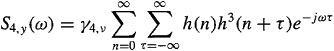
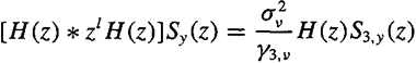
Corollary C-2. Let Ck, y(τ) denote the diagonal slice of the kth-order cumulant, e.g., C3, y (τ) = C3, y(τ1 = τ, τ2 = τ) and Sk, y(ω) is its discrete-time Fourier transform (DTFT). Additionally, let
(C-46)
![]()
Then
(C-47)
![]()
This is a very interesting equation that relates the usual spectrum of a system’s output to a special polyspectrum, Sk, y (ω). It was developed by Giannakis (1987a) and Giannakis and Mendel (1989). Some applications of (C-47) are given later.
Proof. We derive (C-47) for the case when k = 4, leaving the general derivation as an exercise (Problem C-12). From (C-16), we find that
(C-48)
(C-49)
which can be expressed as
(C-50)
![]()
Using DTFT properties, it is straightforward to show that (C-50) can be written as
(C-51)
![]()
Recall that the spectrum of the system’s output is
(C-52)
![]()
Multiply both sides of (C-51) by H(ω), and substitute (C-52) into the resulting equation to see that
(C-53)
![]()
which can be reexpressed as (C-47).![]()
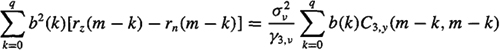
EXAMPLE C-5 GM Equations for MA(q) Systems
For the MA(q) system in (C-25), h(n) = b(n)(n = 1,2,…,q),H2(969;) is the DTFT of b2(n), and H3(ω) is the DTFT of b3(n), so (C-47) can be expressed in the time domain as
(C-54)
![]()
and
(C-55)
![]()
where –q ≤ m ≤ 2q (Problem C-13). These formulas, especially (C-54), have been used to estimate the MA coefficients b(l), b(2),…, b(q) using least-squares or adaptive algorithms (Giannakis and Mendel, 1989; Friedlander and Porat, 1989). Friedlander and Porat refer to these formulas as the “GM equations.” Because they are special cases of (C-47), we prefer to call (C-47) the GM equation.
See Problems C-13 and C-14 for additional aspects of using the GM equations to estimate MA coefficients and an even more general version of the GM equations.![]()
EXAMPLE C-6 Deconvolution
Our system of interest is depicted in Figure C-3. It is single input and single output, causal, linear, and time invariant, in which v(k) is stationary, white, and non-Gaussian with finite variance ![]() nonzero third- or fourth-order cumulant, y 3.v or y4.v, (communication signals are usually symmetrically distributed and, therefore, have zero third-order cumulants); n(k) is Gaussian noise (colored or white); v(k) and n(k) are statistically independent; and H(z) is an unknown asymptotically stable system. Our objective is to design a deconvolution filter in order to obtain an estimate of input v(k). The deconvolution filter is given by θ(z); it may be noncausal.
nonzero third- or fourth-order cumulant, y 3.v or y4.v, (communication signals are usually symmetrically distributed and, therefore, have zero third-order cumulants); n(k) is Gaussian noise (colored or white); v(k) and n(k) are statistically independent; and H(z) is an unknown asymptotically stable system. Our objective is to design a deconvolution filter in order to obtain an estimate of input v(k). The deconvolution filter is given by θ(z); it may be noncausal.
Using the fact that ![]() GM equation (C-47) can be expressed as
GM equation (C-47) can be expressed as
(C-56)
![]()
Figure C-3 Single-channel system and deconvolution filter.

Hence,
(C-57)
![]()
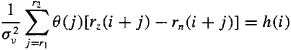
where we have used the fact that, ideally, θ(ω) = l/H(ω). Taking the inverse DTFT of (C-57), using the formula for Hk-1 (ω) in (C-46), we obtain the following interesting relation between H(ω) and its inverse filter 6(co) (Dogan and Mendel, 1994):
(C-58)
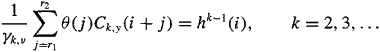
where r1 and r2 are properly selected orders of the noncausal and causal parts of θ(z), respectively.
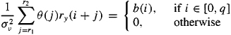
When we have access only to noisy measurements, z(k) = y(k) + n(k), where n(k) is Gaussian and is independent of v(k), then (C-58) becomes
(C-59a)
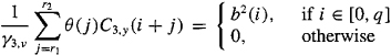
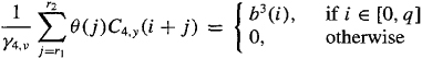
and
(C-59b)

Equation (C-59a) is obtained by using the fact that rz (i+j) = ry (i + j) + rn (i + j). Equation (C-59b) is obtained by using the fact that Ck, n (i + j) = 0, for all k ≥ 3, because n(k) is Gaussian.
Equations (C-58) and (C-59) are applicable to any SISO system, including MA, AR, and ARMA systems. When noisy measurements are available, we must be very careful about using (C-59a), because usually rn (i+j) is unknown. If (C-59a) is used simply by ignoring the rn (i +j) term, errors will be incurred. Such errors do not occur in (C-59b) because the higher-order cumulants have (theoretically) suppressed the additive Gaussian noise.
In the case of an MA(q) system, (C-58) can be expressed as
(C-60)
(C-61)
and
(C-62)
These equations were first derived by Zheng et al. (1993), but in a very different way than our derivation (Problem C-15). They can be used to solve for the deconvolution filter’s coefficients; by choosing i > q, (C-60)-(C-62) become linear in these coefficients. The resulting equations can be solved using least squares. For many numerical examples, see Zheng et al. (1993); their examples demonstrate that in the noisy measurement case it is better to use (C-62) [or (C-61) when third-order cumulants are nonzero] than (C-60), for the reasons described above in connection with (C-59a) and (C-59b).
Finally, we are able to connect the IIR digital Wiener deconvolution filter, described in the Supplementary Material at the end of Lesson 21 (see the section entitled Relationship between Steady-state MVD Filter and an Infinite Impulse Response Digital Wiener Deconvolution Filter) and the cumulant-based deconvolution filter of Example C-6.
Theorem C-2 (Dogan and Mendel, 1994). Under the condition of perfect deconvolution, the deconvolution coefficients determined from (C-59) are optimal in the sense that they are the coefficients that minimize the MSE E{[![]() (k) – v(k)2], when
(k) – v(k)2], when
(C-63)
![]()
and only noisy measurements are available; i.e.,
(C-64)
![]()
regardless of the color of the Gaussian noise, n(k).
Proof. The condition of perfect deconvolution is
(C-65)
![]()
Consider the problem of minimizing E{[![]() ) – v(k2)]}, when
) – v(k2)]}, when ![]() is given by (C-63). This problem was studied in the Supplementary Material at the end of Lesson 21 (see the section entitled Relationship between Steady-state MVD Filter and an Infinite Impulse Response Digital Wiener Deconvolution Filter). Using (21-93), in which z(k) is replaced by y(k), we see that θ(ω) must be chosen so that
is given by (C-63). This problem was studied in the Supplementary Material at the end of Lesson 21 (see the section entitled Relationship between Steady-state MVD Filter and an Infinite Impulse Response Digital Wiener Deconvolution Filter). Using (21-93), in which z(k) is replaced by y(k), we see that θ(ω) must be chosen so that
(C-66)
![]()
Because only z(k) [and not y(k)] is available, we cannot estimate Sy (ω) the best we can do is to estimate S z (a)), where
(C-67)
![]()
Of course, Sn (ω) is unknown to us.
Substitute (C-67) into (C-66) to see that
(C-68)
We now use the GM equation, solving it for Sn (ω). Beginning with (C-47), using (C-67) for Sy (ω), and the fact that Sk, y(ω) = Sk,Z (ω) for all k ≥ 3 [due to the Gaussian nature of n(k)], (C-47) can be expressed as
(C-69)
![]()
Hence,
(C-70)
![]()
Substituting (C-70) into (C-68), we find that
(C-71)
![]()
Applying (C-65) to (C-71), we see that ![]() , or
, or
(C-72)
![]()
From (C-65), we find that l/H(-ω) = θ(-ω). For real signals, H*(ω) = H(ω); hence, (C-72) becomes
(C-73)
![]()
which is exactly the same as (C-57), in which Sk, z(ω) is replaced by Sk, z(ω). From (C-73), we find that
(C-74)
![]()
which is (C-59b).
We have now shown that the IIR WF design equation (C-66) leads to the cumulant-based design equation (C-59b); hence, the cumulant-based deconvolution design is optimal in the mean-squared sense given in the statement of this theorem. ![]()
So far all our results are based on (C-16). What about starting with (C-17)? Two approaches that have done this are worth mentioning. Giannakis and Swami (1987, 1990) have developed a “double C(q, k) algorithm” for estimating the AR and MA coefficients in an ARMA(p, q) model. Their algorithm is derived by starting with (C-17) and inserting the fact that, for an ARMA model, H(z) = B(z)/A(z). By means of some very clever analysis, they then show that both the AR and MA parameters can be determined from a C(q, k) type of equation. See Problem C-16 for some of the details.
The complex cepstrum is widely known in digital signal-processing circles (e.g., Oppenheim and Schafer, 1989, Chapter 12). We start with the transfer function H(z), take its logarithm, ![]() , and then take the inverse z-transform of
, and then take the inverse z-transform of ![]() to obtain the complex cepstrum
to obtain the complex cepstrum ![]() . Associated with
. Associated with ![]() are cepstral coefficients. If they can be computed, then it is possible to reconstruct h(k) to within a scale factor. Starting with (C-17), it is possible to derive a linear system of equations for the cepstral coefficients (Nikias and Pan, 1987; Pan and Nikias, 1988). This method lets us determine the magnitude and phase of a system’s transfer functon using cepstral techniques without the need for phase unwrapping. See Problems C-17 and C-18 for some of the details.
are cepstral coefficients. If they can be computed, then it is possible to reconstruct h(k) to within a scale factor. Starting with (C-17), it is possible to derive a linear system of equations for the cepstral coefficients (Nikias and Pan, 1987; Pan and Nikias, 1988). This method lets us determine the magnitude and phase of a system’s transfer functon using cepstral techniques without the need for phase unwrapping. See Problems C-17 and C-18 for some of the details.
All the higher-order statistical results in Lessons B and C have been for scalar random variables and processes. Extensions of many of these results to vector random variables and processes can be found in Swami and Mendel (1990a) and Mendel (1991). Among their results is a generalization of the Bartlett-Brillinger-Rosenblatt formula (C-16), a generalization in which multiplication [e.g., h(n)h(n + τ)] is replaced by the Kronecker product.
Some additional applications of cumulants to system identification can be found in the problems at the end of this lesson.
Computation
All the M-files that are described next are in the Hi-SpecTM Toolbox (Hi-Spec is a trademark of United Signals and Systems, Inc.). To estimate cumulants or the bispectrum from real data, use:
cumest: Computes sample estimates of cumulants using the overlapped segment method.
bispecd: Bispectrum estimation using the direct (FFT-based) method.
bispeci: Bispectrum estimation using the indirect method.
To compute cumulants for a given single-channel model, use:
cumtrue: Computes theoretical (i.e., true) cumulants of a linear process. This is done using the Bartlett-Brillinger-Rosenblatt formula (C-16). If you also want to compute the theoretical bispectrum of a linear process, first compute the cumulants of that process and then compute the two-dimensional DTFT of the cumulants; or evaluate (C-17) directly.
Determining parameters in AR, MA, or ARMA models can be accomplished using the following Hi-Spec M-files:
arrcest: Estimates AR parameters using the normal equations based on autocorrelations and/or cumulants. See Example C-4.
maest: Estimates MA parameters using the modified GM method. See Example C-5 and Problems C-13 and C-14.
armaqs: Estimates ARMA parameters using the q-slice method. See Example C-3 and Problem C-21.
armarts: Estimates ARMA parameters using the residual time series method. See Problem C-20.
The impulse response of a linear process can be estimated using the bicepstrum method, as described in Problem C-18. This can be accomplished using:
biceps: Nonparametric system identification or signal reconstruction using the bicepstrum method. Computation of the complex cepstrum, by third-order cumulants, without phase unwrapping.
Summary Questions
1. Cumulants are estimated from data by:
(a) numerical integration, as required by the formal definition of expectation
(b) passing the data through a low-pass filter
(c) replacing expectation by sample average
2. The reason it is important to know that sample estimates of cumulants converge in probability to their true values is:
(a) we use functions of cumulants in solutions to many signal-processing problems and can therefore use the consistency carry-over property for these functions
(b) we use functions of cumulants in solutions to many signal-processing problems and can therefore conclude that these functions converge in mean square
(c) it lets us work with short data lengths when we estimate cumulants
3. Which bispectrum estimation method does not first estimate cumulants?
(a) segmentation and averaging
(b) direct method
(c) indirect method
4. The Bartlett-Brillinger-Rosenblatt formulas are important because they:
(a) provide a new way to compute second-order statistics
(b) relate cumulants and polyspectra
(c) generalize our statistical characterization and understanding of the Figure C-1 system from second- to higher-order statistics
5. The Bartlett-Brillinger-Rosenblatt formulas:
(a) only need knowledge of a system’s impulse response
(b) need knowledge of a system’s impulse response and the cumulant of the system’s input
(c) need knowledge of a system’s impulse response and the correlation function of the system’s input
6. The C(q, k) formula lets us determine a channel’s impulse response from:
(a) input and output measurements
(b) only output measurements
(c) only input measurements
7. The output of an AR(p) system is measured in the presence of additive Gaussian noise. Which equations would you use to estimate the p AR coefficients?
(a) correlation-based normal equations
(b) Wiener-Hopf equations
(c) cumulant-based normal equations
8. The GM equation relates:
(a) power spectrum to the DTFT of a diagonal-slice cumulant
(b) power spectrum to the DTFT of the full-blown cumulant
(c) bispectrum to trispectrum
9. A diagonal-slice cumulant relates:
(a) the impulse response of a channel to powers of an inverse filter’s coefficients
(b) inverse filter’s coefficients to powers of the channel’s impulse response
(c) signal to noise
Problems
C-1. Explain in detail how to estimate fourth-order cumulants.
C-2. Here we examine different aspects of ![]() given in Equation (C-3).
given in Equation (C-3).
(a) Verify and explain the meanings of the ranges for s1, and s2 given below Equation (C-3).
(b) Observe that M in the factor 1/M is not equal to the total number of elements in the summation; hence, (C-4) will be biased. Change this factor to ![]() , where
, where ![]() . Prove that
. Prove that ![]() is then an unbiased estimator of
is then an unbiased estimator of ![]()
(c) Prove that ![]() [Hint: max(–a, –b) = – min (a, b).]
[Hint: max(–a, –b) = – min (a, b).]
C-3. In this problem we consider biased correlation estimators. Problem C-4 considers unbiased correlation estimators. Assume that our data are obtained either from M independent realizations, each with a finite number of K samples, or from MK samples from one realization.
(a) Let ![]() denote the following biased segmented correlation estimator:
denote the following biased segmented correlation estimator:
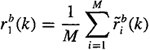
where ![]() denotes the estimated correlation function in the ith segment; i.e.,
denotes the estimated correlation function in the ith segment; i.e.,
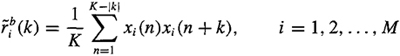
Show that ![]() , where r(k) = E{xi(n)xi(n + k)}, and explain why this estimator is neither unbiased nor asymptotically unbiased.
, where r(k) = E{xi(n)xi(n + k)}, and explain why this estimator is neither unbiased nor asymptotically unbiased.
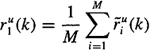
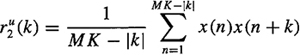
(b) Let ![]() denote an estimator that uses all MK data without segmentation; i.e.,
denote an estimator that uses all MK data without segmentation; i.e.,
![]()
Show that ![]() and explain why this estimator is biased but is asymptotically unbiased.
and explain why this estimator is biased but is asymptotically unbiased.
(c) Compare the biases for ![]() and
and ![]() .
.
(d) Determine formulas for ![]() , and
, and ![]() . Note that this part of the problem will take a very significant effort.
. Note that this part of the problem will take a very significant effort.
C-4. In this problem we consider unbiased correlation estimators. Problem C-3 considers biased correlation estimators. Assume that our data are obtained either from M independent realizations, each with a finite number of K samples, or from MK samples from one realization.
(a) Let ![]() be the unbiased segmented correlation estimator
be the unbiased segmented correlation estimator
where ![]() denotes the estimated correlation function in the ith segment; i.e.,
denotes the estimated correlation function in the ith segment; i.e.,
![]()
Show that ![]() , where r(k) = E{xi(n)xi (n + k)}.
, where r(k) = E{xi(n)xi (n + k)}.
(b) Let ![]() denote an estimator that uses all MK data without segmentation; i.e.,
denote an estimator that uses all MK data without segmentation; i.e.,
Show that ![]() .
.
(c) If you have also completed Problem C-3, then compare ![]() and
and ![]() and
and ![]() and
and ![]() .
.
(d) Determine formulas for ![]() and
and ![]() . Note that this part of the problem will take a very significant effort.
. Note that this part of the problem will take a very significant effort.
C-5. Derive the second-order statistics given in Equations (C-12)–(C-14).
C-6. Complete the details of the derivation of (C-17), starting with (C-16) and (C-21).
C-7. Derive the Bartlett-Brillinger-Rosenblatt equation (C-22), which is valid for the case of a colored non-Gaussian system input, v(k).
C-8. Show that the C(q, k) formula for fourth-order cumulants is
![]()
What is the structure of the C(q, k) formula for fcth-order cumulants?
C-9. Obtain the following formulas for γ3, v and γ4, v, which are by-products of the C(q, k) formula:

and

C-10. Show that (C-36) can be used to compute the MA coefficients b(1), b(2),…, b(q) if we are given all the AR coefficients and only the IR values h(0),h(1),…,h(q).
C-11. This problem explores correlation-based normal equations.
(a) Derive the correlation-based normal equations for the case of noise-free measurements, as stated in (C-42). Do this for both an AR(p) model and an ARMA(p, q) model. Be sure your derivation includes an explanation of the condition m > 0 for the case of an AR(p) model. What is the comparable condition for the ARMA(p, q) model?
(b) Repeat part (a), but for noisy measurements. For an ARMA(p >, q) model and the case of additive white noise, show that
(c) Repeat part (b) but for the case of additive colored noise.
(d) Using the results from parts (b) and (c), explain why measurement noise vastly complicates the utility of the correlation-based normal equations.
[Hints: Operate on both sides of (C-41) with E{-y(n – m)} or E{-z(n – m)}; use the fact that y(n – m) or z(n – m) depends at most on v(n – m).]
C-12. Derive the GM equation (C-47) for arbitrary values of k.
C-13. One method for determining MA coefficients is to use the GM equations of Example C-5, treating both b(i) and b2(i) [or b3(i)] as independent parameters, concatenating (C-54) or (C-55), and then solving for all the unknown b(i) and b2(i) [or b3 (i)] coefficients using least squares. Here we focus on (C-54); comparable results can be stated for (C-55).
(a) Explain why, at most, –q ≤ m ≤ 2q..
(b) Once b(i) and b2(i) have been estimated using least squares, explain two strategies for obtaining ![]() (i), i = 1,2,…,q. Also, explain why this general approach to estimating MA parameters may not give credible results.
(i), i = 1,2,…,q. Also, explain why this general approach to estimating MA parameters may not give credible results.
(c) Suppose only white noisy measurements are available; then GM equation (C-54) becomes
Because we don’t know the variance of the additive white measurement noise, we must remove all the equations to which it contributes. Show that by doing this we are left with an underdetermined system of equations (Tugnait, 1990).
This problem is continued in Problem C-14.
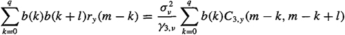
C-14. Tugnait (1990) and Friedlander and Porat (1990) have generalized the GM equation from a diagonal slice to another one-dimensional slice result. We illustrate their results for third-order cumulants.
(a) Set τ1 = τ and τ2 = τ + 1 in (C-16) and obtain the following generalized GM equation (z = ejωτ):
Observe that when l = 0 this equation reduces to (C-47) (for third-order cumulants).
(b) Show that for an MA(g) system the generalized GM equation can be expressed as
Observe that when l = 0 this equation reduces to (C-54).
(c) Set l = q in the formula derived in part (b) to obtain an equation that is almost linear in the unknown MA coefficients. Show that there are 2q + 1 such equations.
(d) How many equations survive when only white noisy measurements are available?
(e) Explain how the remaining equations from part (d) can be combined with those from part (c) of Problem C-13 to provide an overdetermined system of equations that can then be simultaneously solved for b(k) and b2(k), k = 1, 2,…, q.
C-15. In this problem you will derive (C-60) and (C-61) using a very different approach than the GM equation. The approach (Zheng et al., 1993) is to obtain two formulas for Φvy(i) = E{v(k)y(k +i)} (or Φvyy(i) = E{v(k)y2(k + i)}) and to then equate the two formulas. The first formula is one in which y(k) is replaced by its convolutional model, y(k) = v(k) * h(k), whereas the second formula is one in which ![]() is replaced by v(k), where
is replaced by v(k), where ![]() .
.
(a) Derive Equation (C-60).
(b) Derive Equation (C-61).
Note that it is also possible to derive (C-62) by computing Φvyyy(i) = E{v(k)y3, in two ways.
C-16. In this problem we examine the double C(q, k) algorithm, which was developed by Giannakis and Swami (1987, 1990) for estimating the parameters of the ARMA(p, q) system H(z) = B(z)/A(z), where
The double C(q, k) algorithm is a very interesting application of (C-17).
(a) Let ![]() and show that
and show that
(C-16.1)

for (m, n) outside the Figure C-2 six-sided region, where

(b) Starting with (C-16.1) when m = n, obtain a linear system of equations for d(i, j)/d(p, 0) [be sure to use the symmetry properties of d(i, j)]. Show that the number of variables d(i, j)/d(p, 0) is p(p + 3)/2. Explain how you would solve for these variables.
(c) Explain how the C(q, k) algorithm can then be used to extract the AR coefficients.
(d) Show that we can also compute another two-dimensional array of numbers, γ3, vb(m, n), where
and the b(m, n) are related to the MA coefficients of the ARM A model as

(e) Explain how the MA coefficients can then be computed using the C(q, k) algorithm.
The practical application of this double C(q, k) algorithm requires a modified formulation so that steps (c) and (e) can be performed using least squares. See Giannakis and Swami for details on how to do this. Note, finally, that this algorithm is applicable to noncausal as well as to causal channels.
C-17. Different representations of ARMA(p, q) processes are possible. Here we focus on a cascade representation, where H(z) = B(z)/A(z) = cz-rI(z-1)O(z), c is a constant, r is an integer,

is the minimum phase component of H(z), with poles {ci} and zeros {ai} inside the unit circle, i.e., |ci| < 1 and |ai| < 1 for all i, and

is the maximum phase component of H(z), with zeros outside the unit circle at 1/|bi|, where |bi| < 1 for all i. Clearly, h(k) = ci(k) * o(k) * δ(k – r). In this problem we show how to estimate o(k) and i(k), after which h(k) can be reconstructed to within a scale factor and time delay.
Oppenheim and Schafer [1989, Eqs. (12.77) and (12.78)] show i(k) and o(K) can be computed recursively from knowledge of so-called A and B cepstral coefficients, where
In this problem we are interested in how to estimate the cepstral coefficients using higher-order statistics (Nikias and Pan, 1987; Pan and Nikias, 1988).
(a) Beginning with (C-17) for the bispectrum, expressed in the z1 – z2 domain as S3, y,(z1, z2) = γ3, y![]() , take the logarithm of S3, y(z1,Z2),
, take the logarithm of S3, y(z1,Z2), ![]() , and then take the inverse two-dimensional transform of
, and then take the inverse two-dimensional transform of ![]() to obtain the complex bicepstrum by (m, n). To do this, you will need the following power series expansions:
to obtain the complex bicepstrum by (m, n). To do this, you will need the following power series expansions:
and
Show that by (m, n) has nonzero values only at m = n = 0, integer values along the m and n axes and at the intersection of these values along the 45° line m = n; i.e.,
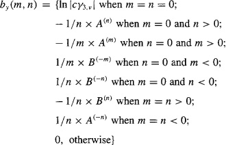
Plot the locations of these complex bicepstral values.
(b) Beginning with (C-17) for the bispectrum, expressed in the z1 – z2 domain as S3, y,(z1, z2) = γ3, y![]() , show that
, show that
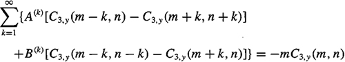
(C-17.1)
![]()
This is a very interesting equation that links the third-order cumulant and the bicepstral values. [Hint: Take the two-dimensional inverse z-transform of ![]()
(c) Using the results from parts (a) and (b), show that
(C-17.2)
(d) Explain why A(k) and B(k) decay exponentially so that A(k) → 0 for k > p1 and B(k) → 0 for k > q1
(e) Truncate (C-17.2) and explain how the A and B cepstral coefficients can be computed using least squares or TLS.
C-18. Here we shall determine second- and third-order statistics for the following three systems (Nikias and Raghuveer, 1987): H1(z) = (1 – az-1)(1 – bz-1), H2(z) = (1 – az)(1 – bz), and H3(z) = (1 – az(1 – bz-1). Note that H1(z) is minimum phase, H2(z) is maximum phase, and H3(z) is mixed phase.
(a) Determine the three autocorrelations r(0), r(1), and r(2) for the three systems. Explain why you obtained the same results for the three systems.
(b) Determine the following third-order cumulants for the three systems: C(0,0), C(1, 0), C(1, 1), C(2, 0), C(2,1), and C(2, 2).
C-19. The residual time-series method for estimating ARMA coefficients is (Giannakis, 1987a, and Giannakis and Mendel, 1989) a three-step procedure: (1) estimate the AR coefficients; (2) compute the residual time series; and (3) estimate the MA parameters from the residual time series. The AR parameters can be estimated using cumulant-based normal equations, as described in Example C-4. The “residual time series,” denoted ![]() , equals
, equals ![]() , where
, where

(a) Letting ![]() , show that the residual satisfies the following equation:
, show that the residual satisfies the following equation:

(b) Explain why ![]() is a highly nonlinear function of the measurements.
is a highly nonlinear function of the measurements.
(c) At this point in the development of the residual time-series method, it is assumed that ![]() , so
, so

Explain how to determine the MA coefficients.
(d) Explain the sources of error in this method.
C-20. The q-slice formula in Example C-3 is the basis for the following q-slice algorithm for determining the coefficients in an ARMA model (Swami, 1988, and Swami and Mendel, 1990b): (1) estimate the AR coefficients; (2) determine the first q IR coefficients using q one-dimensional cumulant slices; and (3) determine the MA coefficients using (C-36). The AR parameters can be estimated using cumulant-based normal equations, as described in Example C-4.
(a) Show that (C-40) can be reexpressed as
![]()
(b) Using the cumulant-based normal equations from Example C-4 and the result in part (a), explain how the AR parameters and scaled values of the IR can be simultaneously estimated.
(c) Explain how we can obtain an estimate of the unsealed IR response values.
(d) Discuss the strengths and weaknesses of this method.