Lesson 25
Maximum-likelihood State and Parameter Estimation

Summary

The purpose of this lesson is to study the problem of obtaining maximum-likelihood estimates of a collection of parameters that appear in our basic state-variable model. A similar problem was studied in Lesson 11; there, state vector x(t) was deterministic, and the only source of uncertainty was the measurement noise. Here, state vector x(t) is random and measurement noise is present as well.

First, we develop a formula for the log-likelihood function for the basic state-variable model. It is in terms of the innovations process; hence, the Kalman filter acts as a constraint that is associated with the computation of the log-likelihood function for the basic state-variable model. We observe that, although we began with a parameter estimation problem, we wind up with a simultaneous state and parameter estimation problem. This is due to the uncertainties present in our state equation, which necessitate state estimation using a Kalman filter.

The only way to maximize the log-likelihood function is by means of mathematical programming. A brief description of the Levenberg-Marquardt algorithm for doing this is given. This algorithm requires the computation of the gradient of the log-likelihood function. The gradient vector is obtained from a bank of Kalman filter sensitivity systems, one such system for each unknown parameter. A steady-state approximation, which uses a clever transformation of variables, can be used to greatly reduce the computational effort that is associated with maximizing the log-likelihood function.

When you complete this lesson, you will be able to use the method of maximum likelihood to estimate parameters in our basic state-variable model.

Introduction

In Lesson 11 we studied the problem of obtaining maximum-likelihood estimates of a collection of parameters, θ = col (elements of Φ, Ψ, H, and R), that appear in the state-variable model

(25-1)

(25-2)

We determined the log-likelihood function to be

(25-3)

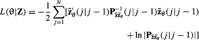
where quantities that are subscripted θ denote a dependence on θ. Finally, we pointed out that the state equation (25-1), written as

(25-4)

acts as a constraint that is associated with the computation of the log-likelihood function. Parameter vector θ must be determined by maximizing L(θ|Z) subject to the constraint (25-4). This can only be done using mathematical programming techniques (i.e., an optimization algorithm such as steepest descent or Levenberg–Marquardt).

In this lesson we study the problem of obtaining maximum-likelihood estimates of a collection of parameters, also denoted 9, that appear in our basic state-variable model,

(25-5)

(25-6)

Now, however,

(25-7)

and we assume that θ is d × 1. As in Lesson 11, we shall assume that θ is identifiable.

Before we can determine , we must establish the log-likelihood function for our basic state-variable model.

A Log-likelihood Function
for the Basic State-variable Model

As always, we must compute p(Z|θ) = p(z(l), z(2),…, z(N)|θ). This is difficult to do for the basic state-variable model, because

(25-8)

The measurements are all correlated due to the presence of either the process noise, w(k), or random initial conditions, or both. This represents the major difference between our basic state-variable model, (25-5) and (25-6), and the state-variable model studied earlier, in (25-1) and (25-2). Fortunately, the measurements and innovations are causally invertible, and the innovations are all uncorrelated, so it is still relatively easy to determine the log-likelihood function for the basic state-variable model.

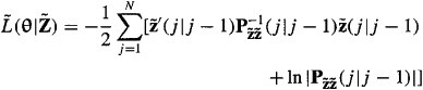
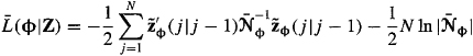
Theorem 25-1. The log-likelihood function for our basic state-variable model in (25-5) and (25-6) is

(25-9)

where is the innovations process, and is the covariance of that process;

(25-10)

This theorem is also applicable to either time-varying or nonstationary systems or both. Within the structure of these more complicated systems there must still be a collection of unknown but constant parameters. It is these parameters that are estimated by maximizing L(θ|Z).

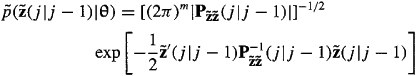
Proof (Mendel, 1983, pp. 101-103). We must first obtain the joint density function p(Z|θ) = p(z(1),…, z(N|θ). In Lesson 17 we saw that the innovations process and measurement z(i) are causally invertible; thus, the density function

contains the same data information as p(z(l),…, z(N|N)|θ) does. Consequently, L(θ|Z) can be replaced by , where

(25-11)

and

(25-12)

Now, however, we use the fact the innovations process is white noise to express as

(25-13)

For our basic state-variable model, the innovations are identically distributed (and Gaussian), which means that for j = 1,…, N; hence,

(25-14)

From part (b) of Theorem 16-2, we know that

(25-15)

Substitute (25-15) into (25-14) to show that

(25-16)

where by convention we have neglected the constant term – ln(2π)^m/2 because it does not depend on θ.

Because and p(#θ) contain the same information about the data, and L(θ|Z) must also contain the same information about the data; hence, we can use L(θ|Z) to denote the right-hand side of (25-16), as in (25-9). To indicate which quantities on the right-hand side of (25-9) may depend on θ, we have subscripted all such quantities with θ.

The innovations process can be generated by a Kalman filter; hence, the Kalman filter acts as a constraint that is associated with the computation of the log-likelihood function for the basic state-variable model.

In the present situation, where the true values of θ, θ_r, are not known but are being estimated, the estimate of x(j) obtained from a Kalman filter will be suboptimal due to wrong values of θ being used by that filter. In fact, we must use in the implementation of the Kalman filter, because will be the best information available about θ_r at t_j If as N → ∞ then as N → ∞, and the suboptimal Kalman filter will approach the optimal Kalman filter. This result is about the best that we can hope for in maximum-likelihood estimation of parameters in our basic state-variable model.

Note, also, that although we began with a parameter estimation problem we wound up with a simultaneous state and parameter estimation problem. This is due to the uncertainties present in our state equation, which necessitated state estimation using a Kalman filter.

On Computing

How do we determine for L(θ|Z) given in (25-9) (subject to the constraint of the Kalman filter)? No simple closed-form solution is possible, because 9 enters into L(θ|Z) in a complicated nonlinear manner. The only way presently known to obtain is by means of mathematical programming.

The most effective optimization methods to determine require the computation of the gradient of L(θ[Z) as well as the Hessian matrix, or a pseudo-Hessian matrix of L(θ|Z). The Levenberg-Marquardt algorithm (Bard, 1970; Marquardt, 1963), for example, has the form

(25-17)

where g_i denotes the gradient

(25-18)

H_i denotes a pseudo-Hessian

(25-19)

and D_i is a diagonal matrix chosen to force H_i + D_i to be positive definite so that (H_i + D_i)^-1 will always be computable.

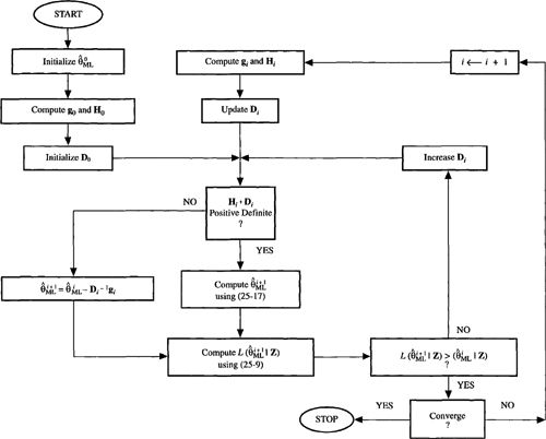
Figure 25-1 depicts a flow chart for the Levenberg-Marquardt procedure. Initial values for must be specified as well as the order of the model, n [for some discussions on how to do this, see Mendel (1990, p. 52), Mendel (1983, pp. 148-149) and Gupta and Mehra (1974)]. Matrix D₀ is initialized to a diagonal matrix. The Levenberg-Marquardt algorithm in (25-17) computes , after which is compared with If we increase D₀ and try again. If then we accept this iteration and proceed to compute using (25-17). By accepting only if we guarantee that each iteration will improve the likelihood of our estimates. This iterative procedure is terminated when the change in falls below some prespecified threshold.

Figure 25-1 Optimization strategy using the Levenberg-Marquardt algorithm. (Adopted from Figure 7.3-1 in J. M. Mendel (1983), Optimal Seismic Deconvolution: An Estimation-based Approach, Academic Press, New York).

Calculations of g_i and H_i, which we describe next, are what is computationally intensive about this algorithm. The gradient of L(θ|Z) is (Problem 25-1)

(25-20)

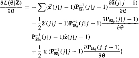
Observe that ∂L(θ|Z)/∂θ requires the calculations of

The innovations depend on ; hence, to compute , we must compute . A Kalman filter must be used to compute ; but this filter requires the following sequence of calculations: . Taking the partial derivative of the prediction equation with respect to θ_i, we find that

(25-21)

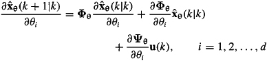
We see that to compute we must also compute Taking the partial derivative of the correction equation with respect to θ_i, we find that

(25-22)

Observe that to compute we must also compute ∂K_θ(k+1)/∂θ_i. We leave it to the reader (Problem 25-2) to show that the calculation of ∂K_θ(k+1)/∂θ_i requires the calculation of ∂P_θ(k+1|k)/∂θ_i which in turn requires the calculation of ∂P_θ(k+1|k+1)/∂θ_i

The system of equations

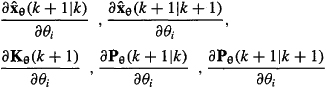
is called a Kalman filter sensitivity system. It is a linear system of equations, just like the Kalman filter, which is not only driven by measurements z(k + 1) [e.g., see (25-22)], but is also driven by the Kalman filter [e.g., see (25-21) and (25-22)]. We need a total of d such sensitivity system, one for each of the d unknown parameters in θ.

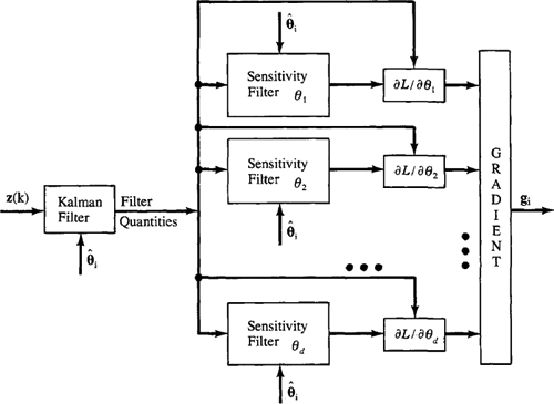
Each system of sensitivity equations requires about as much computation as a Kalman filter. Observe, however, that Kalman filter quantities are used by the sensitivity equations; hence, the Kalman filter must be run together with the d sets of sensitivity equations. This procedure for recursively calculating the gradient ∂L(θ|Z)/∂θ therefore requires about as much computation as d + 1 Kalman filters. The sensitivity systems are totally uncoupled and lend themselves quite naturally to parallel processing (see Figure 25-2).

Figure 25-2 Calculations needed to compute gradient vector g_i. Note that θ_j. denotes the jth component of θ (Mendel, 1983, © 1983, Academic Press, Inc.).

The Hessian matrix of L(θ|Z) is quite complicated, involving not only first derivatives of and , but also their second derivatives. The pseudo-Hessian matrix of L(θ|Z) ignores all the second derivative terms; hence, it is relatively easy to compute because all the first derivative terms have already been computed in order to calculate the gradient of L(θ|Z). Justification for neglecting the second derivative terms is given by Gupta and Mehra (1974), who show that as approaches θ_T the expected value of the dropped terms goes to zero.

The estimation literature is filled with many applications of maximum-likelihood state and parameter estimation. For example, Mendel (1983, 1990) applies it to seismic data processing, Mehra and Tyler (1973) apply it to aircraft parameter identification, and McLaughlin (1980) applies it to groundwater flow.

A Steady-state Approximation

Suppose our basic state-variable model is time invariant and stationary so that exists. Let

(25-23)

and

(25-24)

Log-likelihood function is a steady-state approximation of L(θ|Z). The steady-state Kalman filter used to compute and is

(25-25)

(25-26)

in which K is the steady-state Kalman gain matrix.

Recall that

(25-27)

We now make the following transformations of variables:

(25-28)

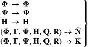
We ignore Γ (initially) for reasons that are explained following Equation (26-33). Let

(25-29)

where Φ is p x 1 and view as a function of Φ; i.e.,

(25-30)

Instead of finding that maximizes , subject to the constraints of a full-blown Kalman filter, we now propose to find that maximizes , subject to the constraints of the following filter:

(25-31)

(25-32)

and

(25-33)

Once we have computed we can compute by inverting the transformations in (25-28). Of course, when we do this, we are also using the invariance property of maximum-likelihood estimates.

Observe that in (25-30) and the filter in (25-31) -(25-33) do not depend on Γ; hence, we have not included Γ in any definition of Φ. We explain how to reconstruct Γ from following Equation (25-45).

Because maximum-likelihood estimates are asymptotically efficient (Lesson 11), once we have determined the filter in (25-31) and (25-32) will be the steady-state Kalman filter.

The major advantage of this steady-state approximation is that the filter sensitivity equations are greatly simplified. When and are treated as matrices of un-known parameters, we do not need the predicted and corrected error-covariance matrices to “compute” and . The sensitivity equations for (25-33), (25-31), and (25-32) are

(25-34)

(25-35)

and

(25-36)

where i = 1,2,…, p. Note that is zero for all Φ_i not in and is a matrix filled with zeros and a single unity value for Φ_i in .

There are more elements in Φ than in θ, because and have more unknown elements in them than do Q and R,_i.e., p > d. Additionally, does not appear in the filter equations; it only appears in . It is, therefore, possible to obtain a closed-form solution for covariance matrix

Theorem 25-2. A closed-form solution for matrix is

(25-37)

Proof. To determine , we must set and solve the

resulting equation for . This is most easily accomplished by applying gradient matrix formulas to (25-30), which are given in Schweppe (1974). Doing this, we obtain

(25-38)

whose solution is in (25-37).

Observe that is the sample steady-state covariance matrix of ; i.e., as

Suppose we are also interested in determining and How do we obtain these quantities from

As in Lessons 19, we let , P_p, and P_f denote the steady-state values of K(k + 1), P(k + l|k), and P(kk), respectively, where

(25-39)

(25-40)

and

(25-41)

Additionally, we know that

(25-42)

By the invariance property of maximum-likelihood estimates, we know that

(25-43)

and>

(25-44)

Solving (25-44) for and substituting the resulting expression into (25-43), we obtain the following solution for :

(25-45)

No closed-form solution exists for. Substituting , , , and into (25-39)-(25-41), and combining (25-40) and (25-41), we obtain

(25-46)

and, from (25-44), we obtain

(25-47)

These equations must be solved simultaneously for P _p and using iterative numerical techniques. For details, see Mehra (1970a).

Note, finally, that the best for which we can hope by this approach is not and , but only . This is due to the fact that, when Γ and Q are both unknown, there will be an ambiguity in their determination; i.e., the term Γw(k) that appears in our basic state-variable model [for which E{w(k)w’(k)} = Q] cannot be distinguished from the term W₁(k), for which

(25-48)

This observation is also applicable to the original problem formulation wherein we obtained directly; i.e., when both Γ and Q are unknown, we should really choose

(25-49)

In summary, when our basic state-variable model is time invariant and stationary, we can first obtain by maximizing given in (25-30), subject to the constraints of the simple filter in (25-31), (25-32), and (25-33). A mathematical programming method must be used to obtain those elements of associated with , , , and The closed-form solution, given in (25-37), is used for Finally, if we want to reconstruct and we use (25-45) for the former and must solve (25-46) and (25-47) for the latter.

EXAMPLE 25-1 (Mehra, 1971)

The following fourth-order system, which represents the short period dynamics and the first bending mode of a missile, was simulated:

(25-50)

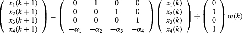
(25-51)

For this model, it was assumed that x(0) = 0, q = 1.0, r = 0.25,α₁ = –0.656, α₂ – 0.784, α₃ = -0.18, and α₄ = 1.0.

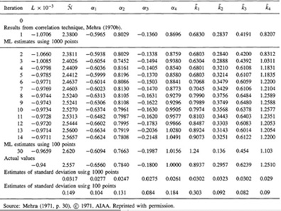
Using measurements generated from the simulation, maximum-likelihood estimates were obtained for Φ, where

(25-52)

In (25-52), is a scalar because, in this example, z(k) is a scalar. Additionally, it was assumed that x(0) was known exactly. According to Mehra (1971, p. 30), “The starting values for the maximum likelihood scheme were obtained using a correlation technique given in Mehra (1970b). The results of successive iterations are shown in Table 25-1. The variances of the estimates obtained from the matrix of second partial derivatives (i.e., the Hessian matrix of ) are also given. For comparison purposes, results obtained by using 1000 data points and 100 data points are given.”

Computation

The Optimization and Control System Toolboxes are very useful to implement portions of maximum-likelihood state and parameter estimators; but neither toolbox has M-files that do everything that is needed for you to implement either a full-blown maximum-likelihood solution or the computationally simpler steady-state approximation.

To implement the full-blown maximum-likelihood solution, you will need to create M-files for Kalman filter sensitivity systems (see Figure 25-2), gradient, pseudo-Hessian, log-likelihood objective function in (25-9), and the Levenberg–Marquardt algorithm as described in the Figure 25-1 flow chart. Our Kalman filter M-file kf (see Appendix B) will also be needed. It is possible that the following M-file, which is in the Optimization Toolbox can be used to directly maximize the log-likelihood function:

Table 25-1 Parameter Estimates For Missile Example

leastsq: Solve nonlinear least squares optimization problems. Its default is the Levenberg–Marquardt algorithm; however, the implementation of this algorithm is very different from the description that we gave in Lessons 25. See the Algorithm section of the software reference manual for the Optimization Toolbox for its description.

To implement the steady-state approximation, you can use our M-file sof (see Appendix B) to implement (25-31)-(25-33), but you will need to create M-files for filter sensitivity systems in (25-34) - (25-36), gradient, pseudo-Hessian, log-likelihood objective function in (25-30), and a Levenberg-Marquardt algorithm that is similar to the one in Figure 25-1. It is also possible that the M-file leastsq can be used to directly maximize the log-likelihood function.

Summary Questions

1. Log-likelihood function in (25-9) depends on θ:

(a) implicitly and explicitly

(b) implicitly

(c) explicitly

2. The log-likelihood function for the basic state-variable model is:

(a) unconstrained

(b) constrained by the state equation

(c) constrained by the Kalman filter

3. To determine for L(θ|Z) in (25-9), we must:

(a) solve a system of normal equations

(b) use mathematical programming

(c) use an EKF

4. The major advantage of the steady-state approximation is that:

(a) the log-likelihood function becomes unconstrained

(b) the filter sensitivity equations are greatly simplified

(c) all parameters can be estimated in closed form

5. For an nth-order system with l unknown parameters, there will be——— Kalman filter sensitivity systems:

(a) l

(b) n

(c) (n+l)/2

6. Matrices Γ and Q, which appear in the basic state-variable model, can:

(a) always be uniquely identified

(b) only be identified to within a constant scale factor

(c) never be uniquely identified

7. The Levenberg-Marquardt algorithm, as presented here, uses:

(a) first- and second-derivative information

(b) only second-derivative information

(c) only first-derivative information

8. The Levenberg-Marquardt algorithm:

(a) converges to a global maximum of L(θ|Z)

(b) will never converge

(c) converges to a local maximum of Z,(θ|Z)

Problems

25-1. Derive the formula for the derivative of the log-likelihood function that is given in (25-20). A useful reference is Kay (1993), pp. 73-74.

25-2. Obtain the sensitivity equations for ∂K_θ (k + 1)/∂θ_i, ∂P_θ (k + 1 |k)/∂θ_i and ∂P_θ (k+1 |k + 1)/∂θ_i. Explain why the sensitivity system for and (k + 1|k + 1)/∂θ_i is linear.

25-3. Compute a formula for H_i. Then simplify H_i to a pseudo-Hessian.

25-4. In thefirst-ordersystem x(k+l) = ax(k)+w(k), and z(k+l) = x(k+l)+v(k+l), k = 1,2,…, N, a is an unknown parameter that is to be estimated. Sequences w(k) and v(k) are, as usual, mutually uncorrelated and white, and w(k) ~ N(w(k); 0, 1) and v(k) ~ N(v(k); 0, ). Explain, using equations and a flow chart, how parameter a can be estimated using a MLE.

25-5. Here we wish to modify the basic state-variable model to one in which w(k) and v(k) are correlated, i.e., E{w(k)v'(k)} = S(k) ≠ 0.

(a) What is θ for this system?

(b) What is the equation for the log-likelihood function L(θ|Z) for this system?

(c) Provide the formula for the gradient of L(θ|Z).

(d) Develop the Kalman filter sensitivity system for this system.

(e) Explain how the preceding results for the modified basic state-variable model are different from those for the basic state-variable model.

25-6. Repeat Problem 25-4 where all conditions are the same except that now w(k) and v(k) are correlated, and .

25-7. We are interested in estimating the parameters a and r in the following first-order system:

x(k + 1) + ax(k) = w(k)

z(k) = x(k) + v(k), k = 1, 2,…,N

Signals w(k) and v(k) are mutually uncorrelated, white, and Gaussian, and E{w²(k)} = 1 and E{n²(k)} = r.

(a) Let θ = col (a, r). What is the equation for the log-likelihood function?

(b) Prepare a macro flow chart that depicts the sequence of calculations required to maximize L(θ|Z). Assume an optimization algorithm is used that requires gradient information about L(θ|Z).

(c) Write out the Kalman filter sensitivity equations for parameters a and r.

25-8. (Gregory Caso, Fall 1991) For the first-order system

x(k + 1) = ax(k) + w(k)

z(k + 1) = x(k + 1) + v(k + 1)

where a, q = E{w²(k)} and E{v²(k)} are unknown:

(a) Write out the steady-state Kalman filter equations.

(b) Write out the steady-state Kalman filter sensitivity equations.

(c) Determine equations for and when the remaining parameters have been estimated.

25-9. (Todd A. Parker and Mark A. Ranta, Fall 1991) The “controllable canonical form” state-variable representation for the discrete-time autoregressive moving average (ARMA) was presented in Example 11-3. Find the log-likelihood function for estimating the parameters of the third-order ARMA system H(z) = [β₁z + β₂]/[z² + α₁z + α₂].

25-10. Develop the sensitivity equations for the case considered in Lessons 11, i.e., for the case where the only uncertainty present in the state-variable model is measurement noise. Begin with L(θ|Z) in (11-42).

25-11. Refer to Problem 23-7. Explain, using equations and a flow chart, how to obtain MLEs of the unknown parameters for:

(a) Equation for the unsteady operation of a synchronous motor, in which C and p are unknown.

(b) Duffing's equation, in which C, α, and β are unknown.

(c) Van der Pol's equation, in which ε is unknown.

(d) Hill's equation, in which a and b are unknown.

25-12. In this lesson, we formulated ML parameter estimation for a state-variable model. Formulate it for the single-input, single-output convolutional model that is described in Example 2-1, Equations (2-2) and (2-3). Assume that input u(k) is zero mean and Gaussian and that the unknown system is MA. You are to estimate the MA parameters as well as the variances of u(k) and n(k).

25-13. When a system is described by an ARMA model whose parameters are unknown and have to be estimated using a gradient-type optimization algorithm, derivatives of the system's impulse response, with respect to the unknown parameters, will be needed. Let the ARMA model be described by the following difference equation:

w(k + n) + a₁w(k + n – 1) +… + a_n-1w(k + 1) + a_nw(k)

=b₁u(k + n - 1) + b₂u(k + n - 2) +…+ b_n-1u(k+ 1) + b_nu(k)

The impulse response is obtained by replacing u(k) by δ(k) and w(k) by h(k); i.e.,

h(k + n) + a₁h(k + n - 1) +… + a_n-1h(k + 1) + a_nh(k)

= b₁δ(k + n - 1)+ b₂δ(k + n - 2) +… + b_n-1δ(k + 1) + b_nδ(k)

For notational simplicity, let A(z) = zⁿ + a₁z^n-1 +… + a_n-1z + a_n and B(z) = b₁z^n-1 + b₂ z^n-2 +… + b_n-1Z + b_n.

(a) Show that ∂h(k)/∂a₁(k = 1,2,…,N) can be obtained by solving the finite difference equation A(z)S_a1(k) = –h(k + n – 1), where sensitivity coefficient s_a1(k) is defined as .

(b) Prove that ∂h(k)/∂a_j = ∂h(k - j + 1)∂a₁ for all j and k. This means that ∂h(k)/∂a_j is obtained from ∂h(k)/∂a₁ simply by shifting the latter's arguments and properly storing the associated values. What is the significance of this result?

(c) Obtain comparable results for ∂h(k)/∂b₁ and ∂h(k)/∂b_j (j = 2,3,…, n and k = 1, 2,…,N).

(d) Flow chart the entire procedure for obtaining s_aj(k) and s_bj(k) for j = 1, 2,… n and k = 1, 2,…,N.

25-14. In Example 14-2 we developed the essence of maximum-likelihood deconvolution. Review that example to see that we assumed that the channel was known. Now let us assume that the channel is unknown. Suppose that the channel is the ARMA model described in Problem 25-13 (the reference for this example is Mendel, 1990).

(a) Show that the results in Example 14-2 remain unchanged, except that objective function M(q|Z) in (14-35) also depends on the unknown ARMA parameters, , and ; i.e., M(q|Z) → M(q, a, b|Z).

(b) Explain why it is not possible to optimize M(q, a, b|Z) simultaneously with respect to q, a, and b.

(c) Because of part (b), we usually maximize M(q, a, b|Z) using a block component method (BCM), in which we initially specify the ARMA parameters and then detect the events; then we optimize the ARMA parameters, after which we redetect the events; and so on until M(q, a, b|Z) does not change appreciably. Flow chart this BCM.

(d) Assume that a gradient algorithm is used to optimize M(q, a, b|Z) with respect to a and b. Explain how you compute ∂Z'Ω^-1Z/∂a_j without computing the inverse of matrix Ω.

(e) Explain, using words, flow charts, and equations, how you compute ∂ M(q, a, b|Z)/∂a and ∂M(q, a, b|Z)/∂b.

(f) Explain why using the convolutional model to maximize M(q, a, b|Z) is a computational nightmare.

(g) Explain how you convert this problem into an equivalent state- variable model and why solving the resulting ML estimation problem is computationally efficient.