Lesson B
Introduction to Higher-order Statistics

Summary

When signals are non-Gaussian, higher than second-order statistics can be very useful. These higher-order statistics are called cumulants and are related to higher-order moments. We prefer to use cumulants rather than higher-order moments because cumulants have some very desirable properties, which moments do not have, that let us treat cumulants as operators.

Higher-order statistics are defined in this lesson. In general, they are multidimensional functions; e.g., third-order statistics are functions of two variables and fourth-order statistics are functions of three variables. Cumulants, which are analogous to cor-relation functions, work directly with signals in the time domain. Polyspectra, which are analogous to the power spectrum, are multidimensional Fourier transforms of cumulants. Fortunately, many important problems can be solved using one or more one-dimensional slices of a higher-order statistic. Additionally, cumulants and polyspectra of stationary random sequences are rich in symmetries, so they only have to be determined over a rather small region of their domains of support.

Six important properties are given for cumulants. Their use lets us apply cumulants to new situations, just as we apply the familiar expectation operator to new situations. One of the most important situations is that of a measurement that equals signal plus noise, where the noise is Gaussian (colored or white). Using the properties of cumulants, we show that the cumulant of this measurement equals the cumulant of just the signal; hence, cumulants boost signal-to-noise ratio. The same is not true for the correlation of this measurement because it is adversely affected by the correlation of the additive noise.

When you complete this lesson, you will be able to (1) define and determine formulas for cumulants; (2) define and determine formulas for polyspectra; (3) understand the relationships between cumulants and moments and why we prefer to work with cumulants; (4) understand the symmetries of cumulants and polyspectra; (5) understand the notion of a one-dimensional slice cumulant; (6) understand and use six important properties of cumulants; and (7) understand why cumulants tend to boost signal-to-noise ratio.

Introduction

Gaussian signals are completely characterized by first- and second-order statistics, because a Gaussian probability density function is completely described by the mean and variance of the signal. We also know that linear transformations of Gaussian signals result in new Gaussian signals. These facts are the basis for many of the techniques described in this book. When signals are non-Gaussian, which is frequently the case in real-world applications, things are not so simple. Even if we knew the signal’s original non-Gaussian probability density function, a linear transformation of the non-Gaussian signal would change the entire nature of the resulting probability density function.

Ideally, we would like to work with the signal’s probability density function. To do so would require knowledge of all the moments of the probability density function, and, in general, this means that we would need to compute an infinite number of moments, something that is impossible to do. What are the alternatives? We could choose to work with just the first- and second-order moments and then stay within the framework of optimal linear estimators, an approach that has been described in Lesson 13; or we could choose to estimate the entire probability density function, an approach that has been briefly described in the Supplementary Material to Lesson 13; or we could choose to work not only with first- and second-order moments, but with some higher-order moments as well. Doing the latter is based on the premise that, when dealing with non-Gaussian signals, we ought to be able to do a better job of estimation (or other types of signal processing) using more than just first- and second-order statistics. This lesson, as well as the next, focuses on the latter approach.

Before we define higher-order moments and their close relations, cumulants, and study important properties of these statistics, let us pause to explain that these lessons are not about the so-called “method of moments.” Around 1900, the statistician Karl Pearson (1936, and references therein) developed the method of moments, which is conceptually simple, but which has very little theoretical justification; i.e., it may give acceptable results sometimes, but frequently it gives very unacceptable results. The method of moments is based on the fact that sample moments (e.g., the sample mean, sample variance, etc.) are consistent estimators of population moments (e.g.,Bury, 1975); hence, for large samples, it is reasonable to expect that the sample moments provide good approximations to the true (population) moments of the probability density function. If we knew the underlying probability density function, which may depend on some unknown parameters, and could express the population moments in terms of these parameters, then we could equate the sample moments to the population moments. If the density function depends on n parameters (e.g., a Gamma density function depends on two parameters), then, if we do this for the first n nonzero moments, we will obtain a system of n equations in n unknowns, which must be solved for the n unknown parameters. Frequently, in signal-processing applications, the probability density function is not known ahead of time; hence, it is impossible to follow this procedure. Additionally, it is not uncommon for the n equations to be nonlinear, in which case their solution is not unique and is difficult to obtain. See Sorenson (1980) and Gallant (1987) for very extensive discussions on the method of moments.

Definitions of Higher-order Statistics

Higher-order statistics can be defined for both stochastic and deterministic signals. Because of our great interest in this book on the former types of signals, we only define higher-order statistics for them. See Nikias and Petropulu (1993) for definitions of higher-order statistics of deterministic signals. Some of the material in this section is taken from Nikias and Mendel (1993) and Mendel (1991).

If {x(k)}, k = 0, ±1, ±2,… is a real stationary discrete-time random sequence and its moments up to order n exist, then (Papoulis, 1991) the nth-order moment function of {x(k)}, is given by

(B-1)

Observe that, because {x (k)} is a stationary sequence, the nth-order moment depends only on the time differences τ₁,τ₂,…,τ_n-1, where τ_i = 0, ±1, ±2,…, for all i. The second-order moment function m_{2, x}(τ₁) is the autocorrelation function, whereas m_{3, x}(τ₁,τ₂) and m_{4, x}τ(₁,τ₂,τ₃) are the third- and fourth-order moments, respectively.

Note that higher-order moments of the sum of two (or more) statistically independent random sequences do not necessarily equal the sum of the higher-order moments of the two (or more) sequences. This makes it difficult to work with higher-order moments in applications, such as signal processing, where random sequences are combined additively. Cumulants, which are related to moments and are defined next, have the very desirable property that cumulants of the sum of two (or more) statistically independent random sequences equal the sum of the cumulants of the two (or more) sequences.

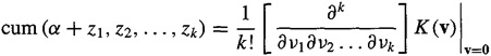
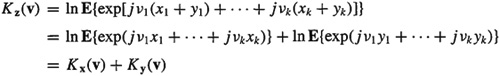
Definition B-l. Let v = col (v₁, v₂,…, vk) and x = col(x₁, x₂,…, x_k), where (x₁, x₂,…, x_k) denotes a collection of random variables. The kth-order cumulant of these random variables is defined (Priestley, 1981) as the coefficient of (v₁v₂…v_k) x j^k in the Taylor series expansion (provided it exists) of the cumulant-generating function

(B-2)

For zero-mean real random variables, the second-, third- and fourth-order cumulants are given by

(B-3a)

(B-3b)

(B-3c)

In the case of nonzero-mean real random variables, we replace x_i by x_i – E{x_i} in these formulas. The case of complexsignals is treated in the references given above and in Problem B-8.

EXAMPLE B-l

Here we derive (B-3a) using (B-2). We leave the comparable derivations of (B-3b) and (B-3c) as a problem for the reader (Problem B-l). According to Definition B-l,

(B-4)

where

(B-5)

Consequently,

(B-6)

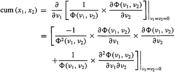
where

(B-7)

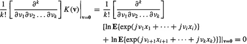
Setting v, = 0 in (B-7), we see that

(B-8)

because the random variables, X_i are zero mean. Note, also, that

(B-9)

Substituting (B-8) and (B-9) into (B-6), we find

(B-10)

where this last result follows (B-7).

The kth-order cumulant is therefore defined in terms of its joint moments of orders up to k. See the Supplementary Material at the end of this lesson for explicit relationships between cumulants and moments.

Definition B-2. Let {x(t)} be a zero-mean kth-order stationary random pro cess. The kth-order cumulant of this process, denoted C_{k, x}(τ₁,τ₂,…τ_k-1) is defined as the joint kth-order cumulant of the random variables x(t), x(t + τ₁),…, x(t + τ_k-1); i.e.,

(B-11)

Because of stationarity, the kth-order cumulant is only a function of the k – 1 lags τ₁,τ₂,…,τ_k-1. If {x(t)} is nonstationary,then the kth-order cumulant depends explicitly on t as well as on τ₁,τ₂…,τ_k-1, and the notation C_{k, x} (t; τ₁,τ₂,…,τ_k-1) can be used.

The second-, third-, and fourth-order cumulants of zero-mean x(t), which follow from (B-3) and (B-11), are

(B-12a)

(B-12b)

(B-12c)

Of course, the second-order cumulant C_{2, x}(τ) is just the autocorrelation of x(t). We shall use the more familiar notation for autocorrelation, r_x (τ), interchangeably with C_{2, x}(τ).

The τ₁ –τ₂ –… τ_k-1space constitutes the domain of support for C_{k, x}(τ₁, τ₂…, τ_{k_1}); i.e., it is where the (k – 1)-dimensional function C_{k, x} (τ₁,τ₂…, τ_k-1) must be evaluated. The domain of support for the autocorrelation function is the one-dimensional real axis. The domain of support for the third-order cumulant function is the two-dimensional τ₁ – τ₂ plane, and the domain of support for the fourth-order cumulant function is the three-dimensional τ₁ – τ₂ – τ₃ volume. Note that a plot of autocorrelation is two-dimensional, a plot of a third-order cumulant is three-dimensional, and a plot of a fourth-order cumulant would be four-dimensional. Naturally, we cannot display the fourth-order cumulant by usual means. Color or sound could be used for the fourth dimension.

EXAMPLE B-2

Here we compute the second- through fourth-order cumulants of the Bernoulli-Gaussian sequence, which we have used in earlier lessons in connection with minimum-variance and maximum-likelihood deconvolution and which is described in Example 13-1. That sequence is

(B-13)

where r (k) is a Gaussian white random sequence, r (k) = N(r (k);0), and q(k) is a Bernoulli sequence for which Pr[q(k) – 1] = λ. Additionally, r(k) and q(k) are statistically independent. Obviously, E{μ(k)} = 0. Due to the whiteness of both r(k) and q(k), as well as their statistical independence, the only higher-order statistics that may be nonzero are those for which all lags are zero. Consequently,

(B-14)

(B-15)

because E{r³(k)} = 0, and

(B-16)

The Bernoulli-Gaussian sequence is one whose third-order cumulant is zero, so we must consequently use fourth-order cumulants when working with it. It is also an example of a higher-order white noise sequence, i.e., a white noise sequence whose second- and higher-order cumulants are multidimensional impulse functions. Its correlation function is nonzero only at the origin of the line of support, with amplitude given by (B-14). Its third-order cumulant is zero everywhere in its plane of support (we could also say that its only possible nonzero value, which occurs at the origin of its two-dimensional domain of support, is zero). Its fourth-order cumulant is nonzero only at the origin of its three-dimensional volume of support, and its value at the origin is given by (B-16).

Equations (B-12) can be used in two different ways: given a data-generating model, they can be used to determine exact theoretical formulas for higher-order statistics of signals in that model; or, given data, they can be used as the basis for estimating higher-order statistics, usually by replacing expectations by sample averages. We shall discuss both of these uses in Lesson C.

For a zero-mean stationary random process and for k = 3,4, the fcth-order cumulant of {x(t)} can also be defined as (Problem B-2)

(B-17)

where M _k.x [x(τ₁),…, x(τ_k-1)] is the kth-order moment function of x(t) and M_{k, g}[gτ₁,…, g(τ_k-1)] is the kth-order moment function of an equivalent Gaussian process, g(t), that has the same mean value and autocorrelation function as x(t). Cumulants, therefore, not only display the amount of higher-order correlation, but also provide a measure of the distance of the random process from Gaussianity. Clearly, if x(t) is Gaussian, then the cumulants are all zero; this is not only true for k = 3 and4, but for all k.

A one-dimensional slice of the kth-order cumulant is obtained by freezing k – 2 of its k – 1 indexes. Many types of one-dimensional slices are possible, including radial, vertical, horizontal, diagonal, and offset diagonal. A diagonal slice is obtained by setting τ_i = τ, i = 1,2, …, k – 1. Some examples of domains of support for such slices are depicted in Figure B-l. All these one-dimensional slices are very useful in applications of cumulants in signal processing.

Figure B-1 Domains of support for one-dimensional cumulant slices of third-order cumulants: (a) vertical slices, (b) horizontal slices, and (c) diagonal and off-diagonal slices.

Many symmetries exist in the arguments of C_{k, x} (τ₁, τ₂,…, τ_k-i), which make the calculations of cumulants manageable. In practical applications, we only work with third- or fourth-order cumulants, because the variances of their estimation errors increase with the order of the cumulant (Lesson C and Nikias and Petropulu, 1993); hence, we only give symmetry conditions for third- and fourth-order cumulants here.

Theorem B-l. (a) Third-order cumulants are symmetric in the following five ways:

(B-18)

(b) Fourth-order cumulants are symmetric in the following 23 ways:

(B-19)

(B-20)

The remaining 15 equalities are obtained by permuting the arguments in the three equalities on the right-hand side of (B-19) five times as in (B-20).

The proof of this theorem works directly with the definitions of the third- and fourth- order cumulants, in (B-12b) and (B-12c), and is left to the reader (Problems B-3 and B-4). Note that the 23 equalities for the fourth-order cumulant are obtained from the 3 equalities in (B-19) plus the 4 x 5 = 20 equalities obtained by applying the 5 equalities in (B-20) to the 4 cumulants in (B-19). See Pflug et al. (1992) for very comprehensive discussions about these symmetry regions.

Using the five equations in (B-18), we can divide the plane into six regions, as depicted in Figure B-2. Knowing the cumulants in any one of these regions, we can calculate the cumulants in the other five regions using these equations. The principal region of support is the first-quadrant 45° sector, 0 . See Pflug et al. (1992, Fig. 9) for a comparable diagram for the 24 regions of symmetry of the fourth-order cumulant. The symmetry relationships for cumulants do not hold in the nonstationary case.

Figure B-2Symmetry regions for third-order cumulants.

If a random sequence is symmetrically distributed, then its third-order cumulant equals zero; hence, for such a process we must use fourth-order cumulants. For example, Laplace, uniform, Gaussian, and Bernoulli-Gaussian distributions are symmetric, whereas exponential, Rayleigh, and k-distributions are nonsymmetric (Problems B-6 and B-7).

EXAMPLE B-3

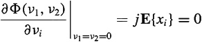
What do cumulants look like? Figure B-3 depicts the impulse response for a tenth-order system, as well as the autocorrelation function, third-order diagonal-slice cumulant, and fourth-order diagonal slice cumulant for that system. Exactly how these results were obtained will be discussed in Lesson C. Whereas autocorrelation is symmetric about the origin [i.e., r_y (–τ) = r_y(τ)], third- and fourth-order diagonal-slice cumulants are not symmetric about their origins. Observe that positive-lag values of the diagonal-slice cumulants have a higher frequency content than do negative lag values and that positive-lag frequency content is greater for fourth-order cumulants than it is for third-order cumulants. The latter is a distinguishing feature of these cumulants, which always differentiates them from each other.

Figure B-3 (a) Impulse response for a SISO system that is excited by non-Gaussian white noise and its associated (b) output autocorrelation, (c) output diagonal-slice third-order cumulant, and (d) output diagonal-slice fourth-order cumulant.

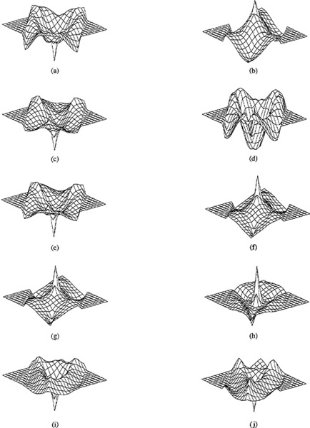
Fourth-order cumulants for this tenth-order system are depicted in Figure B-4. These plots were obtained by first fixing τ₃ and then varying τ₁ and τ₂ from 1 to 9.

Figure B-4 Fourth-order cumulants for the tenth-order system depicted in Figure B-3a. Cumulants C₄,y (τ₁, τ₂, τ₃) –9 ≤ τ₁. τ₂ ≤ 9 are depicted in (a)–(j) for τ₃3 = 0, 1,…, 9. The orientations of the axes are as follows: origin is at the center of the grid; vertical axis is C₄,y(τ₁, τ₂, τ₃) τ₁ axis points to the right; and τ₂ axis points to the left (Swami and Mendel, 1990a, © 1990, IEEE).

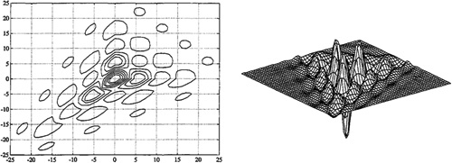
As a second example, Figure B-5 depicts C_{3, y}(τ_1,τ₂) for the ARMA (2, 1) system H (z) = (z – 2) / (z² – 1.5_z + 0.8). The contour plot clearly demonstrates the nonsymmetrical nature of the complete third-order cumulant about the origin of the domain of support. The three-dimensional plot demonstrates that the largest value of the third-order cumulant occurs at the origin of its domain of support and that it can have negative as well as positive values.

Figure B-5 Third-order output cumulant for an ARMA(2, 1) SISO system that is excited by non-Gaussian white noise.

Definition B-3. Assuming that C_{k, x} (τ₁, τ₂,…,τ_k–1) is absolutely summable, the kth-order polyspectrum is defined as the (k-1) -dimensional discrete-time Fourier transform of the kth-order cumulant; i.e.,

(B-21)

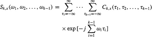
where |ω_i| ≤ π for i = 1, 2,…, k – 1, and |ω₁ + ω₂ +… + ω_{k – 1}|≤ π.

The ω₁ – ω₂ –… –ω_{k – 1} space is the domain of support for S_{k, x} (ω₁, ω₂,…,ω_k–1). s_{3, x} (ω₁,ω₂) is known as the bispectrum [in many papers the notation B_x (ω₁, ω₂) is used to denote the bispectrum], whereas s _{4, x}(ω₁, ω₂, ω₃) is known as the trispectrum.

Theorem B-2. (a) The bispectrum is symmetric in the following 11 ways:

(B-22)

where |ω₁|≤π,|ω₂|≤ π and |ω₁ + ω₂| ≤π, (b) The trispectrum is symmetric in 95 ways, all of which can be found in Pflug et al. (1992), where |ω₁| ≤ π, |ω₂| ≤ π |ω₃ ≤ π, and |ω₁+ω₂+ω₃| ω π

The proof of this theorem works directly with the definitions of bispectrum and trispectrum, which are obtained from (B-21). The reader is asked to prove (B-22) in Problem B-5. Note that if x(t) is complex then S_{3, x} (ω₁, ω₂) is symmetric in only 5 ways [the five unconjugated equations in (B-22)]. When x(t) is real, then so that symmetry occurs in 11 ways.

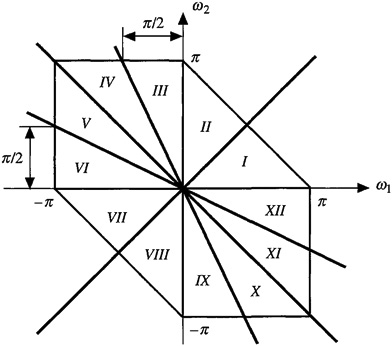
Using the 11 equations in (B-22), we can divide the τ – τ plane into 12 regions, as depicted in Figure B-6. Note that these regions are bounded because of the three inequalities on τ and τ, which are stated just after (B-22). Knowing the bispectrum in any one of these regions, we can calculate the bispectrum in the other 11 regions using (B-22).

Figure B-6 Symmetry regions for the bispectrum.

EXAMPLE B-4

Figure B-7 depicts two different signals that have identical autocorrelation but different third-order statistics. Consequently, these two signals have identical power spectra and different bispectra. Figure (a-1) depicts the zeros of a minimum-phase system; i.e., all the zeros lie inside of the unit circle. Figure (b-1) depicts the zeros of a spectrally equivalent nonminimum-phase system; i.e., some of the zeros from the (a-1) constellation of zeros have been reflected to their reciprocal locations outside of the unit circle. The term spectrally equivalent denotes the fact that the spectrum, which is proportional to , is unchanged when z is replaced by z^-1; hence, when some or all of a minimum-phase H(z)’ zeros are reflected (i.e., z – > z^-1) outside the unit circle (minimum phase → nonminimum phase), remains unchanged.

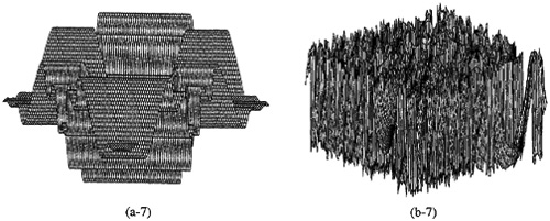
Figure B-7 Comparisons of two systems that have the same power spectra but different bispectra. One system is minimum phase and the other is a spectrally equivalent nonminimum-phase system. See the text of Example B-4 for a description of the many parts of this figure.

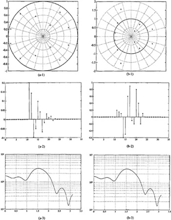
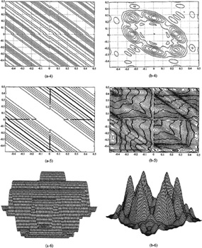
Figures (a-2) and (b-2) depict the impulse responses for the minimum- and nonminimum-phase MA systems. Observe that the IR of the minimum-phase system is “front-loaded” i.e., its maximum value occurs at its front end, whereas the maximum value of the IR of the nonminimum-phase system occurs between its initial and final values. This is a distinguishing feature of minimum- and nonminimum-phase systems.

Figures (a-3) and (b-3) depict the power spectra for the two systems, which of course are identical. We see, therefore, that it is impossible to discriminate between these two systems on the basis of their power spectra, because power spectrum is “phase blind.”

The bispectrum is a complex function of two frequencies, ω₁ and ω₂. A contour of the magnitude of the bispectrum is depicted in (a-4) and (b-4) for the two systems. Examination of these two figures reveals significant differences. A contour of the phase of the bispectrum is depicted in (a-5) and (b-5) for the two systems. Three-dimensional plots of the magnitude and phase of the bispectra for the two systems are given in (a-6) and (a-7) and (b-6) and (b-7), respectively. It is very clear that the phase plots are also markedly different for the two systems. This suggests that it should be possible to discriminate between the two systems on the basis of their bispectra (or their third-order cumulants). We shall demonstrate the truth of this in Lesson C.

Properties of Cumulants

One of the most powerful features of expectation is that it can be treated as a linear operator; i.e., E{ax (k) + by (k)} = a E{x (k)} + bE{y(k)}. Once we have proved this fact, using the probabilistic definition of expectation, we do not have to reprove it every time we are faced with a new situation to which we apply it. Cumulants can also be treated as an operator; hence, they can be applied in a straightforward manner to many new situations. The next theorem provides the bases for doing this.

Theorem B-3. Cumulants enjoy the following properties:

[CP1] If λ_i= 1,…, k, are constants, and x_i, = 1,…, k, are random variables, then

(B-23)

[CP2] Cumulants are symmetric in their arguments; i.e.,

(B-24)

where (i₁,…, i_k) is a permutation of (1,…, k).

[CP3] Cumulants are additive in their arguments; i.e.,

(B-25)

This means that cumulants of sums equal sums ofcumulants (hence, the name “cumulant”).

[CP4] If α is a constant, then

(B-26)

[CP5] If the random variables {x_i} are independent of the random variables {y_i}, i = 1,2…, k, then

(B-27)

[CP6] If a subset of the k random variables {xⁱ} is independent of the rest, then

(B-28)

Proof. A complete proof of this theorem is given in the Supplementary Material at the end of this lesson.

EXAMPLE B-5 (Mendel, 1991)

Suppose z(n) = y(n) + v(n), where y(n) and v(n) are independent; then, from [CP5],

(B-29)

If v(n) is Gaussian (colored or white) and k ≥ 3, then

(B-30)

whereas

(B-31)

This makes higher-order statistics more robust to additive measurement noise than correlation, even if that noise is colored. In essence, cumulants can draw non-Gaussian signals out of Gaussian noise, thereby boosting their signal-to-noise ratios.

It is important to understand that (B-30) is a theoretical result. When cumulants are estimated from data using sample averages, the variances of these estimates are affected by the statistics of the additive noise v(n). See Lesson C for some discussions on estimating cumulants.

Additional applications of Theorem B-3 are given in Lesson C.

Supplementary Material

Relationships between Cumulants and Moments (Mendel, 1991)

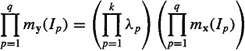
Let x denote a collection of random variables, i.e., X = col (x1, x2,…, x_k), and I_x = {1, 2,…, k}, denote the set of indexes of the components of x. If then X_i is the vector consisting of those components of x whose indexes belong to I. We denote the simple moment and cumulant of the subvector X_i of the vector x as m_x(I) [i.e., m_x(I) is the expectation of the product of the elements in x_i] and C_x(I). The partition of the set I is the unordered collection of nonintersecting nonempty sets I_psuch that . For example, the set of partitions corresponding to k = 3 is {(1, 2, 3)}, {(1),(2, 3)},{(2), (1, 3)}, {(3), (1, 2)}, {(1), (2), (3)}.

The moment-to-cumulant (i.e., M-C) formula is [Leonov and Shiryaev (1959)]

(B-32)

where denotes summation over all partitions of set I. In the preceding example, q = 1 for {(1, 2, 3)}, q = 2 for {(1), (2, 3)}, {(2), (1, 3)}, and {(3), (1, 2)}, and q = 3 for {(1), (2), (3)}. The cumulant-to-moment (i.e., C-M) equation is [Leonov and Shiryaev (1959)]

(B-33)

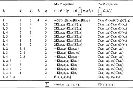
An example that illustrates the use of (B-32) and (B-33) for I = {1, 2, 3,4} is given in Table B-1. In its bottom row, Σ means add all preceding rows to obtain either cum {(x₁, x₂, x₃, x₄)}, using (B-32), or E{(₁x₂x₃x₄)} using (B-33).

Proof of Theorem B-3 (Mendel, 1991)

Property [CP1]: Let y = col (λ₁x₁,…, λ_kx_k), and x = col (x₁,…, x_k). Note that (see previous section) I_x = I_y From (B-32), we see that

(B-34)

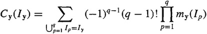
Table B-1 CALCULATIONS OF FOURTH-ORDER CUMULANTS IN TERMS OF MOMENTS AND VICE VERSA (MENDEL, 1991)

where [for example, apply the results in Table B-1 to y = col (λ₁x₁, λ₂x₂, λ₃x₃, λ₄x₄)]

(B-35)

Consequently,

(B-36)

which is (B-23).

Property [CP2]: Referring to (B-32), since the partition of the set I_x is an unordered collection of nonintersecting nonempty sets of I_p such that _x, the order in the cumulant’s argument is irrelevant to the value of the cumulant. As a result, cumulants are symmetric in their arguments.

Property [CP3]: col(u₁+ v₁, x₂,…,x_k) where u = col(u₁, x₂,…,x_k) and v = col(v₁, x₂,…, x_k). Observe that [because m_x(I_i) is the expectation of the product of the elements in I_i and u₁ + v₁ appears only raised to the unity power]

(B-37)

Substitute (B-37) into (B-32) to obtain the result in (B-25).

Property [CP4]: Let y = col (α + z₁, z₂,…, z_k); then, from (B-2), we see that

(B-38)

According to the paragraph that precedes (B-2), we know that

(B-39)

but, from (B-38), we see that

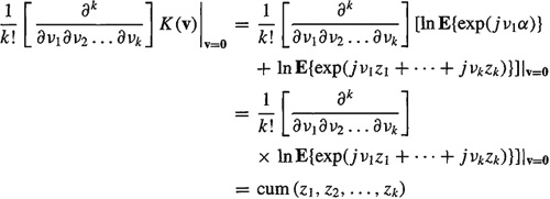
which is (B-26).

Property [CP5]: Let z = col(x₁ + y₁,…,x_k + y_k) = x + y, where x = col (x₁,…, x_k) and y = col (y₁,…, y_k) Using the independence of the {x_i} and {y_i}, it follows that

(B-40)

from which the result in (B-27) follows directly.

Property [CP6]: Assume that (x₁,…, x_i) is independent of (x_i+1,…, x_k);

hence,

(B-41)

Now

which is (B-28).

Summary Questions

1. Cumulants and moments are:

(a) always the same

(b) never the same

(c) sometimes the same

2. The domain of support for C_k,_x(τ₁, τ₂,…, τ_k-1) is the:

(a) τ₂ - τ₁, τ₃ - τ₁,…,τ_k-1 - τ₁ soace

(b) t, τ₁, τ₂, τ_k-1 space

(c) τ₁, τ₂,…,τ_k-1 space

3. Cumulants not only display the amount of higher-order correlation, but also provide a measure of:

(a) non-Gaussianity

(b) the distance of the random process from Gaussianity

(c) causality

4. Symmetries, which exist in the arguments of C_{k, x}(τ₁, τ₂,…,τ_k-1):

(a) are only useful in theoretical analyses

(b) are only valid for k = 3

(c) make the calculations of Cumulants manageable

5. The bispectrum is the discrete-time Fourier transform of the:

(a) fourth-order cumulant

(b) third-order cumulant

(c) correlation function

6. In general, cumulants are preferrable to higher-order moments, because:

(a) cumulants of two (or more) statistically independent random sequences equal the sum of the cumulants of the two (or more) sequences, whereas the same is not necessarily true for higher-order moments

(b) cumulants are easier to compute than higher-order moments

(c) odd-order cumulants of symmetrically distributed sequences equal zero

7. Cumulants are said to “boost signal-to-noise ratio” because:

(a) cum(signal + non-Gaussian noise) = cum(signal) + cum(non-Gaussian noise)

(b) cum(signal + Gaussian noise) = cum(signal)

(c) cum(signal + Gaussian noise) = cum(signal) × cum(Gaussian noise)

8. Cumulants and moments can:

(a) never be determined from one another

(b) sometimes be determined from one another

(c) always be determined from one another

9. Cumulant properties:

(a) let us treat the cumulant as an operator

(b) always have to be reproved

(c) are interesting, but are of no practical value

Problems

B-l. Derive Equations (B-3b) and (B-3c) using Equation (B-2).

B-2. Beginning with Equation (B-17), derive the third- and fourth-order cumulant formulas that are given in Equations (B-12b) and (B-12c).

B-3. Derive the symmetry conditions given in Equation (B-18) for the third-order cumulant C_{3, x}(τ₁, τ₂). Then explain how Figure B-2 is obtained from these conditions.

B-4. Derive the symmetry conditions given in Equations (B-19) and (B-20) for the fourth-order cumulant C_{4, x}(τ₁, τ₂, τ₃).

B-5. Derive the bispectrum symmetry conditions that are given in Equation (B-22). Then explain how Figure B-5 is obtained from these conditions.

B-6. Consider a random variable x that is exponentially distributed; i.e., its probability density function is p(x) = λe^-λx u_-1(x). Let m_{i, x} and C_{i, x} denote the ith-order moment and cumulant, respectively, for x. Show that (Nikias and Petropulu, 1993): m_{1, x} = 1/λ, m_{2, x} = 2/λ², m_{3, x} = 6/λ³, m_{4, x} = 24/λ⁴ and C_{1, x} = 1/λ, C_{2, x} = 1/λ², C_{3, x} = 2/λ³, C_{4, x} = 6/λ⁴. For comparable results about Rayleigh or K- distributed random variables, see page 11 of Nikias and Petropulu (1993).

B-7. Consider a random variable x that is Laplace distributed; i.e., its probability density function is p(x) = 0.5e,^-|x|. Let m_{i, x} and C_{i, x} denote the ith-order moment and cumulant, respectively, for x. Show that (Nikias and Petropulu, 1993): m_{1, x} = 0, m_{2, x} = 2, m_3,x = 0, m_4,x = 24, and C_{1, x} = 0, C_2,x = 2, C_3,x = 0, C_4,x = 12. For comparable results about Gaussian or uniformly distributed random variables, see page 10 of Nikias and Petropulu (1993). Note that for these three distributions x is “symmetrically distributed” so that all odd-order moments or cumulants equal zero.

B-8. Let a = exp(jφ), where φ is uniformly distributed over [ -π, π].

(a) Show that all third-order cumulants of complex harmonic a are always zero.

(b) Show that, of the three different ways (different in the sense of which of the variables should be conjugated) to define a fourth-order cumulant of a complex harmonic, only one always yields a nonzero value; i.e., cum (a, a, a, a) = 0, cum (a^*, a, a, a) = 0, but cum (a^*, a^*, a, a) = -1. These results suggest that the fourth-order cumulant of the complex random sequence {y(n)}, should be defined as

C_{4, y}(τ₁, τ₂, τ₃ = cum (y^*(n), y^*(n + τ₁), y(n + τ₂, y(n + τ₃))

(c) Explain why it doesn’t matter which two of the four arguments in this definition are conjugated.

B-9. Let S = exp(jφ), where φ is uniformly distributed over [ -π, π], and let a₁(l = 0, 1, 2, 3) be constants. Prove that (Swami, 1988)

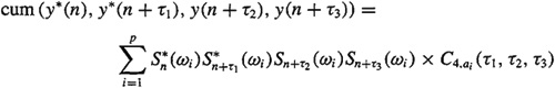
B-10. A model that can be used to describe a wide range of problems is (Prasad et al., 1988)

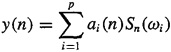
where the S_n(.)’s are signal waveshapes, ω_i’s are constants, and the a_i’s are zero mean and mutually independent, with fourth-order cumulant C_{4, aj}(τ₁, τ₂, τ₃). Show that

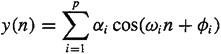
In the harmonic retrieval problem for complex signals, the model is

where the _i’s are independent identically distributed random variables uniformly distributed over [-ππ], wii ≠ j and the a,’s and w_i,’s are constants (i.e., not random). Given measurements of y(n), the objective is to determine the number of harmonics, p, their frequencies, w_i, and their amplitudes, α_i-

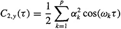
(a) Derive the following formula for the autocorrelation of y(n):

(b) Show that C_{3, y}(τ₁, τ₂ = 0; hence, we must use fourth-order cumulants in this application.

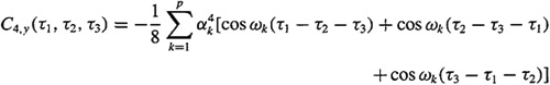
(c) Derive the following formula for C_{4, y}(τ₁, τ₂, τ₃ (Swami and Mendel, 1991):

[Hint: Use the result of Problem B-10, with B-10, with S_n(W_i)= exp(jnw_i,) and α_i = α_i exp(j_i.]

(d) Now assume that only the noise-corrupted measurements z(n)= y(n) + v(n) are available, where v(n) is Gaussian colored noise. Determine formulas for C_{2, z}(τ)and C4,Z(τ₁,τ₂,τ₃). Explain why any method for determining the unknown parameters that is based on fourth-order cumulants will still work when we have access only to z(n), whereas a method based on second-order statistics will not work when we have access only to z(n).

Observe that when τ₁ τ₂ = τ₃ the equation for C_{4, y}(τ_,τ_,τ)looks very similar to the equatiion for C₂, y(τ). Thissuggests that a method for determining p, W_i and τ, that is based on second-order statistics can also be applied to C_{4, y}(τ,τ,τ). See Swami and Mendel (1991) for details on how to do this.

B-12.In the harmonic retrieval problem for real signals, the model is

where the are independent identically distributed random variables uniformly distributed over [ππ], thefrequencies are distinct, and the α_i’s and ω_i’s are constants (i.e., not random). Given measurements of y(n), the objective is to determine the number of harmonics, p, their frequencies, w_i, and their amplitudes,α_i.

(a) Derive the following formula for the autocorrelation of y(n):

(b) Show that C_{3, y}(τ₁,τ₂) = 0; hence, we must use fourth-order cumulants in this application.

(c) Derive the following formula for C_{4, y}(τ₁,τ₂,τ₃) (Swami and Mendel, 1991):

[Hint: Express each cosine function as a sum of two complex exponentials, and use the results of Problems B-10 and B-9.]

(d) Now assume that only the noise-corrupted measurements z(n) = y(n) + v(n) are available, where v(n) is Gaussian colored noise. Determine formulas for C_{2, z} and C_4,Z(τ₁,τ₂,τ₃). Explain why any method for determining the unknown parameters that is based on fourth-order cumulants will still work when we have access only to z(n), whereas a method based on second-order statistics will not work when we have access only to z(n).

Observe that when τ₁ =τ₂ = τ₃ the equation for C_{4, y} looks very similar to the equation for C _{2, y} (τ). This suggests that a method for determining p, w_i, and α_i that is based on second-order statistics can also be applied to C_{4, y}(τ,τ,τ). See Swami and Mendel (1991) for details on how to do this.

B-13. We are given two measurements, x (n)= S(n) + w_i (n) and y(n)= AS(n-D) + w 2 (n), where S(n) is an unknown random signal and W₁(n)and w ₂ (n) are Gaussian noise sources. The objective in this time delay estimation problem is to estimate the unknown time delay, D [Nikias and Pan (1988)].

(a) Assume that w₁ (n) and w₂ (n) are uncorrelated, and show that r_xy (τ) = E{x(n)y(n + τ)} = r_ss (τ-D). This suggests that we can determine D by locating the time at which the cross-correlation function r_xy(τ) is a maximum.

(b) Now assume that w₁(n) and ₂(n) are correlated and Gaussian, and show that r_xy(τ) = r_ss(τ-D)+r₁₂(τ), where r₁₂(τ) is the cross-correlation function between w₁(n) and w₂ (n). Because this cross-correlation is unknown, the method stated in part (a) for determining D won’t work in the present case.

(c) Again assume that w₁(n) and w₂(n) are correlated and Gaussian, and show that the third-order cross-cumulant . Then show that S_xyx(ω₁ω2) = S_3,S(ω₁, ω₂2) exp(–jω₁ D) and S_xxx(ω₁, ω₂) = S_{3, s}(ω₁, ω₂). Suggest a method for determining time-delay D from these results. Observe that the approach in this part of the problem has been able to handle the case of correlated Gaussian noises, whereas the second-order statistics-based approach of part (b) was not able to do it.