Lesson 15
Elements of Discrete-time Gauss-Markov Random Sequences

Summary

This is another transition lesson. Prior to studying recursive state estimation, we first review an important body of material on discrete-time Gauss-Markov random sequences. Most if not all of this material should be a review for a reader who has had courses in random processes and linear systems.

A first-order Markov sequence is one whose probability law depends only on the immediate past value of the random sequence; hence, the infinite past does not have to be remembered for such a sequence.

It is in this lesson that we provide a formal definition of Gaussian white noise. We also introduce the basic state-variable model. It consists of a state equation and a measurement equation and can be used to describe time-varying nonstationary systems. Of course, it is a simple matter to specialize this model to time-invariant and stationary systems, simply by making all the time-varying matrices that appear in the state-variable model constant matrices. The basic state-variable model is not the most general state-variable model; however, it is a simple one to use in deriving recursive state estimators. Lesson 22 treats more general state-variable models.

Many statistical properties are given for the basic state-variable model. They require that all sources of uncertainty in that model must be jointly Gaussian. One important result from this lesson is a procedure for computing the mean vector and covariance matrix of a state vector using recursive formulas.

Finally, we define the important concept of signal-to-noise ratio and show how it can be computed from a state-variable model.

When you complete this lesson, you will be able to (1) state many useful definitions and facts about Gauss-Markov random sequences; (2) define Gaussian white noise; (3) explain the basic state-variable model and specify its properties; (4) use recursive algorithms to compute the mean vector and covariance matrix for the state vector for our basic state-variable model; and (5) define signal-to-noise ratio and explain how it can be computed.

Introduction

Lesson 13 and 14 have demonstrated the importance of Gaussian random variables in estimation theory. In this lesson we extend some of the basic concepts that were introduced in Lessons 12, for Gaussian random variables, to indexed random variables, that is, random sequences. These extensions are needed in order to develop state estimators.

Definition and Properties of Discrete-time Gauss-Markov Random Sequences

Recall that a random process is a collection of random variables in which the notion of time plays a role.

Definition 15-1 (Meditch, 1969, p. 106). A vector random process is a family of random vectors {s(t), t ∈ } indexed by a parameter t all of whose values lie in some appropriate index set . When = {k : k = 0,1,…} we have a discrete-time random sequence.

Definition 15-2 (Meditch, 1969, p. 117). A vector random sequence {s(t), t ∈ } is defined to be multivariate Gaussian if, for any ℓ time points t₁, t₂,…, t_e in , where ℓ is an integer, the set of ℓ random n vectors s(t₁), s(t₂),…, s(t_ℓ), is jointly Gaussian distributed.

Let S(ι) be defined as

(15-2)

Then Definition 15-2 means that

(15-2)

in which

(15-3)

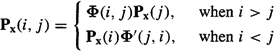
and P_s(ι) is the nl x nl matrix E{[S(ι) – m_s(ι)][S(ι) – m_s(ι)]′} with elements P_s(i, j), where

(15-4)

i, j = 1,2,…, l.

Definition 15-3 (Meditch, 1969, p. 118). A vector random sequence {s(t), t ∈, } is a Markov sequence, if, for any m time points t₁. < t₂ <… < t_m in , where m is any integer, it is true that

(15-5)

For continuous random variables, this means that

(15-6)

Note that, in (15-5), s(t_m) ≤ S(t_m) means s_i(t_m) ≤ S_i(t_m) for i = 1, 2,…, n. If we view time point t_m as the present time and time points t_m-1,…, t₁ as the past, then a Markov sequence is one whose probability law (e.g., probability density function) depends only on the immediate past value, t_m-1. This is often referred to as the Markov property for a vector random sequence. Because the probability law depends only on the immediate past value, we often refer to such a process as a first-order Markov sequence (if it depended on the immediate two past values it would be a second-order Markov sequence).

Theorem 15-1. Let {s(t), t ∈ } be a first-order Markov sequence, and t₁ < t2 <… < t_m be any time points in , where m is an integer. Then

(15-7)

Proof. From probability theory (e.g., Papoulis, 1991) and the Markov property of s(t), we know that

(15-8)

In a similar manner, we find that

(15-9)

Equation (15-7) is obtained by successively substituting each of the equations in (15-9) into (15-8).

Theorem 15-1 demonstrates that a first-order Markov sequence is completely characterized by two probability density functions; the transition probability density function p[s(t_i)|s(t_i–1)] and the initial (prior) probability density function p[s(t₁)]. Note that generally the transition probability density functions can all be different, in which case they should be subscripted [e.g., p_m [s(t_m)|s(t_m–1)] and P_m–1[S(t_m–1)|S(t_m–2)]].

Theorem 15-2. For a first-order Markov sequence,

(15-10)

We leave the proof of this useful result as an exercise.

A vector random sequence that is both Gaussian and a first-order Markov sequence will be referred to in the sequel as a Gauss-Markov sequence.

Definition 15-4. A vector random sequence {s(t), t ∈ } is said to be a (discrete-time) Gaussian white sequence if, for any m time points t₁, t₂,… t_m in , where m is any integer, the m random vectors s(t₁), s(t₂),…, s(t_m) are uncorrelated Gaussian random vectors.

White noise is zero mean, or else it cannot have a flat spectrum. For white noise

(15-11)

Additionally, for Gaussian white noise

(15-12)

[because uncorrelatedness implies statistical independence (see Lesson 12)], where p[s(t_i] is a multivariate Gaussian probability density function.

Theorem 15-3. A vector Gaussian white sequence s(t) can be viewed as a firstorder Gauss-Markov sequence for which

(15-13)

for all t, τ ∈, and t ≠ τ.

Proof. For a Gaussian white sequence, we know from (15-12), that

(15-14)

But we also know that

(15-15)

Equating (15-14) and (15-15), we obtain (15-13).

Theorem 15-3 means that past and future values of s(t) in no way help determine present values of s(_t). For Gaussian white sequences, the transition probability density function equals the marginal density function, p[s(t)], which is multivariate Gaussian. Additionally (Problem 15-1),

(15-16)

Definition 15-5. A vector random sequence {s(t), t ∈ } is strictly stationary if its probability density function is the same for all values of time. It is wide-sense stationary if its first- and second-order statistics do not depend on time.

The Basic State-variable Model

In succeeding lessons we shall develop a variety of state estimators for the following basic linear, (possibly) time-varying, discrete-time, dynamical system (our basic state-variable model), which is characterized by n x 1 state vector x(k) and m x 1 measurement vector z(k):

(15-17)

and

(15-18)

where k = 0,1,… In this model w(k) and v(k) are p x 1 and m x 1 mutually uncorrelated (possibly nonstationary) jointly Gaussian white noise sequences; i.e.,

(15-19)

(15-20)

and

(15-21)

Covariance matrix Q(i) is positive semidefinite and R(i) is positive definite [so that R^-1(i) exits]. Additionally, u(k) is an l x 1 vector of known system inputs, and initial state vector x(0) is multivariate Gaussian, with mean m_x(0) and convariance P_x(0);i.e.,

(15-22)

and x(0) is not correlated with w(k) and v(k). The dimensions of matrices Φ, Γ, Ψ, H, Q, and R are n x n, n x p, n x l, m x n, p x p, and m x m, respectively.

Comments

1. The double arguments in matrices Φ, Γ, and Ψ may not always be necessary, in which case we can replace (k + 1, k) by (k). This will be true if the underlying system, whose state-variable model is described by (15-17) and (15-18), is discrete time in nature. When the underlying system is continuous time in nature, it must first be discretized, a process that is described in careful detail in Lesson 23 (in the section entitled “Discretization of Linear Time-varying State-variable Model”), where you will learn that, as a result of discretization, the matrices Φ, Γ, and Ψ do have the double arguments (k + l, k). Because so many engineering systems are continuous time in nature and will therefore have to first be discretized, we adopt the double argument notation in this book.

2. In Lesson 11 we used the notation for E{v(k)v′(k)}; here we use R. In the earlier lessons, the symbol R was reserved for the covariance of the noise vector in our generic linear model. Because state estimation, which is the major subject in the rest of this book, is based on the state-variable model and not on the generic linear model, there should be no confusion between our use of symbol R in state estimation and its use in the earlier lessons.

3. I have found that many students of estimation theory are not as familiar with state-variable models as they are with input/output models; hence, I have included a very extensive introduction to state-variable models and methods as a supplementary lesson (Lesson D).

4. Disturbance w(k) is often used to model the following types of uncertainty:

a. disturbance forces acting on the system (e.g., wind that buffets an airplane);

b. errors in modeling the system (e.g., neglected effects); and

c. errors, due to actuators, in the traslation of the known input, u(k), into physical signals.

5. Vector v(k) is often used to model the following types of uncertainty:

a. errors in measurements made by sensing instruments;

b. unavoidable disturbances that act directly on the sensors; and

c. errors in the realization of feedback compensators using physical components [this is valid only when the measurement equation contains a direct throughput of the input u(k), i.e., when z(k + 1) = H(k + 1)x(k + 1) + G(k+ 1)u(k + 1) + v(k + 1); we shall examine this situation in Lesson 22].

6. Of course, not all dynamical systems are described by this basic model. In general, w(k) and v(k) may be correlated, some measurements may be made so accurate that, for all practical purposes, they are “perfect” (i.e., no measurement noise is associated with them), and either w(k) or v(k), or both, may be colored noise processes. We shall consider the modification of our basic state-variable model for each of these important situations in Lessons 22.

Properties of the Basic State-variable Model

In this section we state and prove a number of important statistical properties for our basic state-variable model.

Theorem 15-4. When x(0) and {w(k), k = 0, 1,…} are jointly Gaussian, then x(k), k = 0, 1…} is a Gauss-Markov sequence.

Note that if x(0) and w(k) are individually Gaussian and statistically independent (or uncorrelated), they will be jointly Gaussian (Papoulis, 1991).

Proof

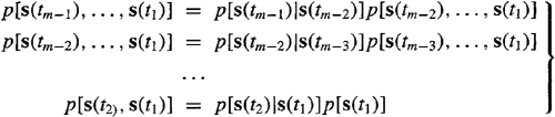
a. Gaussian property [assuming u(k) nonrandom]. Because u(k) is nonrandom, it has no effect on determining whether x(k) is Gaussian; hence, for this part of the proof, we assume u(k) = 0. The solution to (15-17) is (Problem 15-2)

(15-23)

where

(15-24)

Observe that x(k) is a linear transformation of jointly Gaussian random vectors x(0), w(0), w(1)…, w(k – 1); hence, x(k) is Gaussian.

b. Markov property. This property does not require x(k) or w(k) to be Gaussian. Because x satisfies state equation (15-17), we see that x(k) depends only on its immediate past value; hence, x(k) is Markov.

We have been able to show that our dynamical system is Markov because we specified a model for it. Without such a specification, it would be quite difficult (or impossible) to test for the Markov nature of a random sequence.

By stacking up x(1), x(2)…, into a supervector, it is easily seen that this super-vector is just a linear transformation of jointly Gaussian qualities x(0), w(0), w(1),… (Problem 15-3); hence, x(1), x(2),… are themselves jointly Gaussian.

A Gauss-Markov sequence can be completely characterized in two ways:

1. Specify the marginal density of the initial state vector, p[x(0)], and the transition density p[x(k + 1)|x(k)].

2. Specify the mean and covariance of the state vector sequence.

The second characterization is a complete one because Gaussian random vectors are completely characterized by their means and covariances (Lesson 12). We shall find the second characterization more useful than the first.

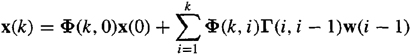
The Gaussian density function for state vector x(k) is

(15-25)

where

(15-26)

and

(15-27)

We now demonstrate that m_x(k) and P_x(k) can be computed by means of recursive equations.

Theorem 15-5. For our basic state-variable model:

a. m_x(k) can be computed from the vector recursive equation

(15-28)

where k = 0, 1,…, and m_x (0) initializes (15-28).

b. P_x(k) can be computed from the matrix recursive equation

(15-29)

where k = 0, 1,…, and Px(0) initializes (15-29).

c. can be computed from

(15-30)

Proof

a. Take the expected value of both sides of (15-17), using the facts that expectation is a linear operation (Papoulis, 1991) and w(k) is zero mean, to obtain (15-28).

b. For notational simplicity, we omit the temporal arguments of4> and F in this part of the proof. Using (15-17) and (15-28), we obtain

(15-31)

Because m_x(k is not random and W(k) is zero mean, E{m_x(k)w’ (k)} = m_xE{w’(k)} = 0, and E{w(k)mx’(k)} = 0. State vector x(k) depends at most on random input w(k – 1) [see (15-17)]; hence,

(15-32)

and E{w(k)x’ (k)} = 0 as well. The last two terms in (15-31) are therefore equal to zero, and the equation reduces to (15-29).

c. We leave to proof of (15-30) as an exercise. Observe that once we know covariance matrix P_x(k) it is an easy matter to determine any cross-covariance matrix between state x(k) and x(i)(≠ k). The Markov nature of our basic state-variable model is responsible for this.

Observe that mean vector m_x(k) satisfies a deterministic vector state equation, (15-28), covariance matrix P_x(k) satisfies a deterministic matrix state equation, (15-29), and (15-28) and (15-29) are easily programmed for digital computation.

Next we direct our attention to the statistics of measurement vector z(k).

Theorem 15-6. For our basic state-variable model, when x(0), w(k), and v(k) are jointly Gaussian, then {z(k), k = 1, 2,…} is Gaussian, and

(15-33)

and

where m_x(k+ 1) and P x(k+1) are computed from (15-28) and (15-29), respectively

We leave the proof as an exercise for the reader. Note that if x(0), w(k), and v(k) are statistically independent and Gaussian they will be jointly Gaussian.

EXAMPLE 15-1

Consider the simple single-input, single-output first-order system

(15-35)

(15-36)

where w(k) and v(k) are wide-sense stationary white noise processes, for which q = 20 and r = 5. Additionally, m _x(0) = 4 and p x (0) = 10.

The mean of x(k) is computed from the following homogeneous equation:

(15-37)

and the variance of x(k) is computed from Equation (15-29), which in this case simplifies to

(15-38)

Additionally, the mean and variance of z(k) are computed from

(15-39)

and

(15-40)

Figure 15-1 depicts m_x (k) and . Observe that m _x (k) decays to zero very rapidly and that approaches a steady-state value . This steady-state value can be computed from Equation (15-38) by setting The existence of is guaranteed by our first-order system being stable.

Figure 15-1 Mean (dashed) and standard deviation (bars) for first-order system (15-35) and (15-36).

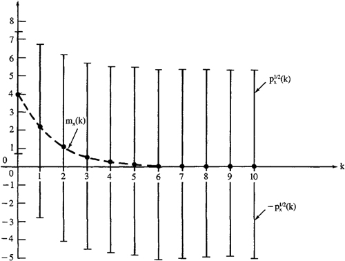
Although m _x (k) –> 0, there is a lot of uncertainty about x(k), as evidenced by the large value of There will be an even larger uncertainty about z(k), because These large values for and are due to the large values of q and r. In many practical applications, both q and r will be much less than unity, in which case and will be quite small.

For our basic state-variable model to be stationary, it must be time invariant, and the probability density functions of w(k) and v(k) must be the same for all values of time (Definition 15-5). Because w(k) and v(k) are Gaussian, this means that Q(k) must equal the constant matrix Q and R(k) must equal the constant matrix R. Additionally, either x(0) = 0 or Φ(k, 0)x(0) ≈ 0 when k > k₀ [see (15-23)]. In both cases x k will be in its “steady-state” regime, so stationarity is possible.

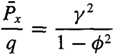
If our basic state-variable model is time invariant and stationary and if Φ is associated with an asymptotically stable system (i.e., one whose poles all lie within the unit circle), then (Anderson and Moore, 1979) matrix P K (k) reaches a limiting (steady-state) solution Px; i.e.,

Figure 15-1 Mean (dashed) and standard deviation (bars) for first-order system (15-35) and (15-36).

(15-41)

Matrix is the solution of the following steady-state version of (15-29):

(15-42)

This equation is called a discrete-time Lyapunov equation. See Laub (1979) for an excellent numerical method that can be used to solve (15-42) for .

Signal-to-Noise Ratio

In this section we simplify our basic state- variable model (15-17) and (15-18) to a time-invariant, stationary, two-input, single-output model:

(15-43)

(15-44)

Measurement z(k) is of the classical form of signal plus noise, where “signal” s(k)=h’x(k)

The signal-to-noise ratio is an often-used measure of quality of measurement z(k). Here we define that ratio, denoted by SNR(k), as

(15-45)

From preceding analyses, we see that

(15-46)

Because P_x(k) is in general a function of time, SNR(k) is also a function of time. If, however, Φ is associated with an asymptotically stable system, then (15-41) is true. In this case we can use in (15-46) to provide us with a single number, , for the signal-to-noise ratio; i.e.,

(15-47)

Finally, we demonstrate that SNR(k) (or ) can be computed without knowing q and r explicitly; all that is needed is the ratio q/r. Multiplying and dividing the right-hand side of (15-46) by q, we find that

(15-48)

Scaled covariance matrix P_x(k)/q is computed from the following version of (15-29):

(15-49)

One of the most useful ways for using (15-48) is to compute q/r for a given signal-to-noise ratio ; i.e.,

(15-50)

In Lesson 18 we show that q/r can be viewed as an estimator tuning parameter; hence, signal-to-noise ratio, , can also be treated as such a parameter.

EXAMPLE 15-2 (Mendel, 1981)

Consider the first-order system

(15-51)

(15-52)

In this case, it is easy to solve (15-49) to show that

(15-53)

Hence,

(15-54)

Observe that if h²y² = 1 – ² then = q/r. The condition h²y² = 1 – ² is satisfied if, for example, y = 1, = 1/, and h = 1/.

Computation

This lesson as well as its companion lesson, Lesson E, are loaded with computational possibilities. The Control System Toolbox contains all the M-files listed next except eig, which is a MATLAB M-file.

Models come in different guises, such as transfer functions, zeros and poles, and state variable. Sometimes it is useful to be able to go from one type of model to another. The following Model Conversion M-files will let you do this:

ss2tf: State space to transfer function conversion.

ss2zp: State space to zero pole conversion.

tf2ss: Transfer function to state space conversion.

tf2zp: Transfer function to zero pole conversion.

zp2tf: Zero pole to transfer function conversion.

zp2ss: Zero pole to state space conversion.

Once a model has been established, it can be used to generate time responses. The following time response M-files will let you do this:

dlsim: Discrete-time simulation to arbitrary input.

dimpulse: Discrete-time unit sample response.

dinitial: Discrete-time initial condition response.

dstep: Discrete-time step response.

Frequency responses can be obtained from:

dbode: Discrete Bode plot. It computes the magnitude and phase response of discrete-time LTI systems.

Eigenvalues can be obtained from:

ddamp: Discrete damping factors and natural frequencies.

eig: eigenvalues and eigenvectors.

There is no M-file that lets us implement the full-blown time-varying state-vector covariance equation in (15-29). If, however, your system is time invariant and stationary, so that all the matrices associated with the basic state-variable model are constant, then the steady-state covariance matrix of x(k) [i.e., the solution of (15-42)] can be computed using:

dcovar: Discrete (steady-state) covariance response to white noise.

Summary Questions

1. A first-order Markov sequence is one whose probability law depends:

(a) on its first future value

(b) only on its immediate past value

(c) on a few past values

2. Gaussian white noise is:

(a) biased

(b) uncorrelated

(c) colored

3. The basic state-variable model is applicable:

(a) to time-varying and nonstationary systems

(b) only to time-invariant and nonstationary systems

(c) only to time-varying and stationary systems

4. If no disturbance is present in the state equation, then:

(a) m_x (k + 1) = Φm_x(k)

(b) P_x(i, j) = I for all i and j

(c) P_x(k + 1) = ΦP_x(k + 1) = Φ'

5. A steady-state value of P_x (k) exists if our system is:

(a) time invariant and has all its poles inside the unit circle

(b) time varying and stable

(c) time invariant and has some of its poles outside the unit circle

6. In general, signal-to-noise ratio is:

(a) always a constant

(b) a function of time

(c) a polynomial in time

7. If measurements are perfect, then:

(a) P_z (k + 1) = HP_x (k + 1)H'

(b) Q = 0

(c) m_z (k + 1) = 0

8. Which statistical statements apply to the description of the basic state-variable model?

(a) w(k) and v(k) are jointly Gaussian

(b) w(k) and v(k) are correlated

(c) w(k) and v(k) are zero mean

(d) Q(k) > 0

(e) R(k) > 0

(f) x(0) is non-Gaussian

9. {x(k), k = 0, 1,…} is a Gauss-Markov sequence if x(0) and w(k) are:

(a) independent

(b) jointly Gaussian

(c) uncorrelated

10. A random sequence is a (an)___________ family of random variables:

(a) large

(b) Markov

(c) indexed

11. To compute signal-to-noise ratio for a two-input single-output model, we need to know:

(a) both q and r

(b) q but not r

(c) just q/r

12. A first-order Markov sequence is completely characterized by which probability density functions?

(a) p[s(t₁)]

(b) p[s(t_i|t₁)]

(c) p[s(t_i|s(t_i-1)]

Problems

15-1. Prove Theorem 15-2, and then show that for Gaussian white noise E{s(t_m)|s(t_m-1),…, s(t₁)} = E{s(t_m)}.

15-2. (a) Derive the solution to the time-varying state equation (15-17) that is given in (15-23).

(b) The solution in (15-23) expresses x(k) as a function of x(0); derive the following solution that expresses x(k) as a function of x(j), where j < k:

15-3. In the text it is stated that “By stacking up x(1), x(2),… into a supervector it is easily seen that this supervector is just a linear transformation of jointly Gaussian quantities x(0), w(0), w(1),…; hence, x(1), x(2),… are themselves jointly Gaussian?.” Demonstrate the details of this “stacking” procedure for x(1), x(2), and x(3).

15-4. Derive the formula for the cross-covariance of x(k), P_x(i, j) given in (15-30). [Hint: Use the solution to the state equation that is given in part (b) of Problem 15-2.]

15-5. Derive the first- and second-order statistics of measurement vector z(k), that are summarized in Theorem 15-6.

15-6. Reconsider the basic state-variable model when x(0) is correlated with w(0), and w(k) and v(k) are correlated [E{w(k)v'(k)} = S(k)].

(a) Show that the covariance equation for z(k) remains unchanged.

(b) Show that the covariance equation for x(k) is changed, but only at k = 1.

(c) Compute E{z(k + l)z'(k)}.

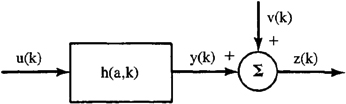
15-7. In this problem, assume that u(k) and v(k) are individually Gaussian and uncorrelated. Impulse response h depends on parameter a, where a is a Gaussian random variable that is statistically independent of u(k) and v(k).

(a) Evaluate E{z(k)}.

(b) Explain whether or not y(k) is Gaussian.

Figure P15-7

15-8. (Kiet D. Ngo, Spring, 1992) White noise is very useful in theoretical studies; however, it usually does not exist in real physical systems. The typical noise in physical systems is colored. A first-order Gauss-Markov process x(k) has an autocorrelation function and spectral density . Find the transfer function of the filter that will shape a unity-variance Gaussian white noise process into a first-order Gauss-Markov process whose autocorrelation and spectral density are as given. Draw the block diagram of the filter.

15-9. (Mike Walter, Spring 1992) Consider the following system:

where w(k) and v(k) are wide-sense stationary white noise processes, m_x (0) = 0, m_x(1) = 0, and q = 25.

(a) Find a basic state-variable model for this system.

(b) Find the steady-state values of E{x²(k)} and E{x(k + l)x(k)}.

15-10. (Richard S. Lee, Jr., Spring 1992) Consider the following measurement equation for the basic state-variable model:

z(k + 1) = H(k + 1)x(k + 1) + v(k + 1)

where x(k + 1) = col (x₁(k + 1), x₂(k + 1):

w(k) and v(k) are mutually uncorrelated, zero-mean, jointly Gaussian white noise sequences, and E{w(i)w(j)} = δ_{i, j}.

(a) Determine the state equation of the basic state-variable model.

(b) Given that E{x₁(0)} = E{x₂ (0)} = 0, u(0) = 1, u(1) = 0.5, and P_x (0) = I, find m_x (1), m_x(2), P_x(1), and P_x(2).

15-11. (Lance Kaplan, Spring 1992) Suppose the basic state-variable model is modified so that x(0) is not multivariate Gaussian but has finite moments [in this problem, u(k) is deterministic].

(a) Is x(k), in general, multivariate Gaussian for any k ≥ 0?

(b) Now let Φ(k + 1, k) = Φ, where all the eigenvalues of Φ have magnitude less than unity. What can be said about the multivariate probability density function of x (k) as k becomes large?

(c) What are the mean and covariance of x(k) as k approaches infinity?

(d) Let = lim x(k) as k → ∞. Does the distribution of depend on the initial condition x(0)?

15-12. (Iraj Manocheri, Spring 1992) Consider the state equation

where x(0) = 2, E{u(k)} = 1, and cov [u(k)] = δ(k₂ – k₁).

(a) Find the recursions for the mean and covariance of x(k).

(b) Find the steady-state mean and covariance of x(k).