Lesson 16
State Estimation: Prediction
Summary
Prediction, filtering, and smoothing are three types of mean-squared state estimation that have been developed during the past 35 years. The purpose of this lesson is to study prediction.
A predicted estimate of a state vector x(k) uses measurements that occur earlier than tk and a model to make the transition from the last time point, say tj, at which a measurement is available to tk. The success of prediction depends on the quality of the model. In state estimation we use the state equation model. Without a model, prediction is dubious at best.
Filtered and predicted state estimates are very tightly coupled together; hence, most of the results from this lesson cannot be implemented until we have developed results for mean-squared filtering. This is done in Lessons 17.
A single-stage predicted estimate of x(k) is denoted ![]() It is the mean-squared estimate of x(k) that uses all the measurements up to and including the one made at time tk-1; hence, a single-stage predicted estimate looks exactly one time point into the future. This estimate is needed by the Kalman filter in Lessons 17.
It is the mean-squared estimate of x(k) that uses all the measurements up to and including the one made at time tk-1; hence, a single-stage predicted estimate looks exactly one time point into the future. This estimate is needed by the Kalman filter in Lessons 17.
The difference between measurement z(k) and its single-stage predicted value, ![]() , is called the innovations process. This process plays a very important role in mean-squared filtering and smoothing. Interestingly enough, the innovations process for our basic state-variable model is a zero-mean Gaussian white noise sequence.
, is called the innovations process. This process plays a very important role in mean-squared filtering and smoothing. Interestingly enough, the innovations process for our basic state-variable model is a zero-mean Gaussian white noise sequence.
When you complete this lesson, you will be able to (1) derive and use the important single-stage predictor; (2) derive and use more general state predictors; and (3) explain the innovations process and state its important properties.
Introduction
We have mentioned, a number if times in this book, that in state estimation three situations are possible depending on the relative relationship of total number of available measurements, N, and the time point, k, at which we estimate state vector x(k): prediction (N < k), filtering (N = k), and smoothing (N > k). In this lesson we develop algorithms for mean-squared predicted estimates, ![]() of state x(k). To simplify our notation, we shall abbreviate
of state x(k). To simplify our notation, we shall abbreviate ![]() as
as ![]() [Just in case you have forgotten what the notation
[Just in case you have forgotten what the notation ![]() stands for, see Lesson 2]. Note that, in prediction, k > j.
stands for, see Lesson 2]. Note that, in prediction, k > j.
Single-stage Predictor
The most important predictor of x(k) for our future work on filtering and smoothing is the single-stage predictor ![]() . From the fundamental theorem of estimation theory (Theorem 13-1), we know that
. From the fundamental theorem of estimation theory (Theorem 13-1), we know that
(16-1)
![]()
where
(16-2)
![]()
It is very easy to derive a formula for ![]() by operating on both sides of the state equation
by operating on both sides of the state equation
(16-3)
![]()
with the linear expectation operator ![]() Doing this, we find that
Doing this, we find that
(16-4)
![]()
where k = 1,2,…. To obtain (16-4), we have used the facts that ![]() and u(k – 1) is deterministic.
and u(k – 1) is deterministic.
Observe, from (16-4), that the single-stage predicted estimate ![]() depends on the filtered estimate
depends on the filtered estimate ![]() of the preceding state vector x(k – 1). At this point, (16-4) is an interesting theoretical result; but there is nothing much we can do with it, because we do not as yet know how to compute filtered state estimates. In Lesson 17 we shall begin our study into filtered state estimates and shall learn that such estimates of x(k) depend on predicted estimates of x(k), just as predicted estimates of x(k) depend on filtered estimates of x(k – 1); thus, filtered and predicted state estimates are very tightly coupled together.
of the preceding state vector x(k – 1). At this point, (16-4) is an interesting theoretical result; but there is nothing much we can do with it, because we do not as yet know how to compute filtered state estimates. In Lesson 17 we shall begin our study into filtered state estimates and shall learn that such estimates of x(k) depend on predicted estimates of x(k), just as predicted estimates of x(k) depend on filtered estimates of x(k – 1); thus, filtered and predicted state estimates are very tightly coupled together.
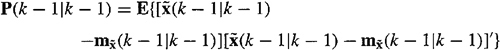
Let ![]() denote the error-covariance matrix that is associated with
denote the error-covariance matrix that is associated with ![]() ; i.e.,
; i.e.,
(16-5)
where
(16-6)
![]()
Additionally, let ![]() denote the error-covariance matrix that is associated with
denote the error-covariance matrix that is associated with![]() ; i.e.,
; i.e.,
(16-7)
For our basic state-variable model (see Property 1 of Lesson 13), ![]() and
and ![]() , so
, so
(16-8)
![]()
and
(16-9)
![]()
Combinin (16-3) and (16-4), we see that
(16-10)
![]()
A straightforward calculation leads to the following formula for ![]() :
:
(16-11)
![]()
where k = 1,2,….
Observe, from (16-4) and (16-11), that ![]() and
and ![]() initialize the single-stage predictor and its error covariance. Additionally,
initialize the single-stage predictor and its error covariance. Additionally,
(16-12)
![]()
and
(16-13)
![]()
Finally, recall (Property 4 of Lesson 13) that both ![]() and
and ![]() are Gaussian.
are Gaussian.
A General State Predictor
In this section we generalize the results of the preceding section so as to obtain predicted values of x(k) that look further into the future than just one step. We shall determine ![]() where k > j under the assumption that filtered state estimate
where k > j under the assumption that filtered state estimate ![]() and its error-covariance matrix
and its error-covariance matrix ![]() are known for some j = 0,1,….
are known for some j = 0,1,….
Theorem 16-1
a. If input u(k) is deterministic, or does not depend on any measurements, then the mean-squared predicted estimator x(k), ![]() , is given by the expression
, is given by the expression
(16-14)

b. The vector random sequence ![]() , k = j + 1, j + 2,…} is:
, k = j + 1, j + 2,…} is:
i. zero mean
ii. Gaussian, and
iii. first-order Markov, and
iv. its covariance matrix is governed by
(16-15)
![]()
Before proving this theorem, let us observe that the prediction formula (16-14) is intuitively what we would expect. Why is this so? Suppose we have processed all the measurements z(l), z(2),…, z(j) to obtain ![]() and are asked to predict the value of x(k), where k > j. No additional measurements can be used during prediction. All that we can therefore use is our dynamical state equation. When that equation is used for purposes of prediction, we neglect the random disturbance term, because the disturbances cannot be measured. We can only use measured quantities to assist our prediction efforts. The simplified state equation is
and are asked to predict the value of x(k), where k > j. No additional measurements can be used during prediction. All that we can therefore use is our dynamical state equation. When that equation is used for purposes of prediction, we neglect the random disturbance term, because the disturbances cannot be measured. We can only use measured quantities to assist our prediction efforts. The simplified state equation is
(16-16)
![]()
a solution of which is (see Problem 15-2b)
(16-17)
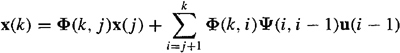
Substituting ![]() for x(y), we obtain the predictor in (16-14). In our proof of Theorem 16-1, we establish (16-14) in a more rigorous manner.
for x(y), we obtain the predictor in (16-14). In our proof of Theorem 16-1, we establish (16-14) in a more rigorous manner.
Proof
a. The solution to state equation (16-3), for x(k), can be expressed in terms of x(j), where j < k, as (see Problem 15-2b)
(16-18)
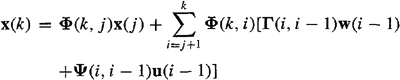
We apply the fundamental theorem of estimation theory to (16-18) by taking the conditional expectation with respect to Z(j) on both sides of it. Doing this, we find that
(16-19)

Note that Z(j) depends at most on x(j), which, in turn, depends at most on w(j – 1). Consequently,
(16-20)
![]()
where i = j + 1, j + 2,…,k. Because of this range of values on argument i, w(i – 1) is never included in the conditioning set of values w(0), w(1),…, w(j – 1); hence,
(16-21)
![]()
for all i = j + 1, j + 2,…, k.
Note, also, that
(16-22)
![]()
because we have assumed that u(i – 1) does not depend on any of the measurements. Substituting (16-21) and (16-22) into (16-19), we obtain the prediction formula (16-14).
b(i) and b(ii). Have already been proved in Properties 1 and 4 of Lessons 13.
b(iii). Starting with ![]() and substituting (16-18) and (16-14) into this relation, we find that
and substituting (16-18) and (16-14) into this relation, we find that
(16-23)

This equation looks quite similar to the solution of state equation (16-3), when u(k) = 0 (for all k), e.g., see (16-18); hence, ![]() also satisfies the state equation
also satisfies the state equation
(16-24)
![]()
Because ![]() depends only on its previous value,
depends only on its previous value, ![]() , it is first-order Markov.
, it is first-order Markov.
b(iv). We derived a recursive covariance equation for x(k) in Theorem 15-5. That equation is (15-29). Because ![]() satisfies the state equation for x(k), its covariance
satisfies the state equation for x(k), its covariance ![]() is also given by (15-29). We have rewritten this equation as in (16-15).
is also given by (15-29). We have rewritten this equation as in (16-15).![]()
Observe that by setting j = k – 1 in (16-14) we obtain our previously derived single-stage predictor ![]() .
.
Theorem 16-1 is quite limited because presently the only values of ![]() and
and ![]() that we know are those at j = 0. For j = 0, (16-14) becomes
that we know are those at j = 0. For j = 0, (16-14) becomes
(16-25)
The reader might feel that this predictor of x(k) becomes poorer and poorer as k gets farther and farther away from zero. The following example demonstrates that this is not necessarily true.
EXAMPLE 16-1
Let us examine prediction performance, as measured by ![]() for the first-order system
for the first-order system
(16-26)
![]()
where q = 25 and px(0) is variable. Quantity ![]() which in the case of a scalar state vector is a variance, is easily computed from the recursive equation
which in the case of a scalar state vector is a variance, is easily computed from the recursive equation
(16-27)
![]()
for k = 1, 2,…. Two cases are summarized in Figure 16-1. When px(0) = 6, we have relatively small uncertainty about ![]() , and, as we expected, our predictions of x(k) for k ≥ 1 do become worse, because
, and, as we expected, our predictions of x(k) for k ≥ 1 do become worse, because ![]() > 6 for all k ≥ 1. After a while,
> 6 for all k ≥ 1. After a while, ![]() reaches a limiting value equal to 50. When this occurs, we are estimating
reaches a limiting value equal to 50. When this occurs, we are estimating ![]() by a number that is very close to zero, because
by a number that is very close to zero, because ![]() approaches zero for large values of k.
approaches zero for large values of k.
Figure 16-1 Prediction error variance ![]() .
.
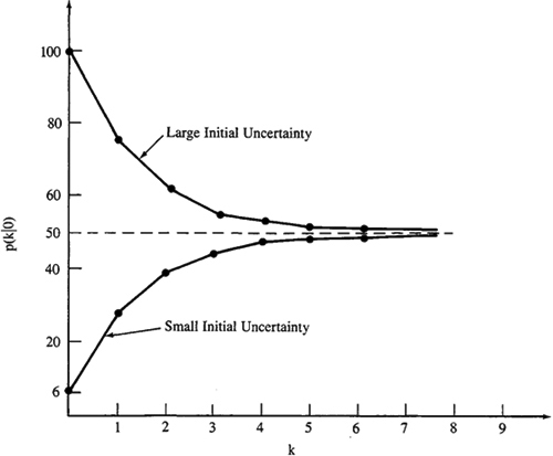
When px(0) = 100, we have large uncertainty about ![]() , and, perhaps to our surprise, our predictions of
, and, perhaps to our surprise, our predictions of ![]() improve in performance, because
improve in performance, because ![]() < 100 for all k ≥ 1. In this case the predictor discounts the large initial uncertainty; however, as in the former case,
< 100 for all k ≥ 1. In this case the predictor discounts the large initial uncertainty; however, as in the former case, ![]() again reaches the limiting value of 50.
again reaches the limiting value of 50.
For suitably large values of k, the predictor is completely insensitive to px(0). It reaches a steady-state level of performance equal to 50, which can be predetermined by setting ![]() and p(k –1/0) equal
and p(k –1/0) equal ![]() , in (16-27), and solving the resulting equation for
, in (16-27), and solving the resulting equation for ![]() .
.![]()
Prediction is possible only because we have a known dynamical model, our state-variable model. Without a model, prediction is dubious at best (e.g., try predicting tomorrow’s price of a stock listed on any stock exchange using today’s closing price).
The Innovations Process
Suppose we have just computed the single-stage predicted estimate of x(k+1),![]() Then the single-stage predicted estimate of z(k + 1),
Then the single-stage predicted estimate of z(k + 1),![]() is
is
![]()
or
(16-28)
![]()
The error between ![]() ; i.e.,
; i.e.,
(16-29)
![]()
Signal ![]() is often referred to either as the innovations process, prediction error process, or measurement residual process. We shall refer to it as the innovations process, because this is most commonly done in the estimation theory literature (e.g., Kailath, 1968). The innovations process plays a very important role in mean-squared filtering and smoothing. We summarize important facts about it in the following:
is often referred to either as the innovations process, prediction error process, or measurement residual process. We shall refer to it as the innovations process, because this is most commonly done in the estimation theory literature (e.g., Kailath, 1968). The innovations process plays a very important role in mean-squared filtering and smoothing. We summarize important facts about it in the following:
Theorem 16-2 (Innovations)
a. The following representations of the innovations process z(k + l|k) are equiva-lent:
(16-30)
![]()
(16-31)
![]()
or
(16-32)
![]()
b. The innovations is a zero-mean Gaussian white noise sequence, with
(16-33)
![]()
a. Substitute (16-28) into (16-29) to obtain (16-31). Next, substitute the measurement equation z(k + 1) = H(k + 1)x(k + 1) + v(k + 1) into (16-31), and use the fact that ![]() to obtain (16-32).
to obtain (16-32).
b. Because ![]() and v(k + 1) are both zero mean,
and v(k + 1) are both zero mean, ![]() . The innovations is Gaussian because z(k + 1) and
. The innovations is Gaussian because z(k + 1) and ![]() are Gaussian, and therefore
are Gaussian, and therefore ![]() is a linear transformation of Gaussian random vectors. To prove that
is a linear transformation of Gaussian random vectors. To prove that ![]() is white noise, we must show that
is white noise, we must show that
(16-34)
![]()
We shall consider the cases i > j and i = j leaving the case i < j as an exercise for the reader. When i > j,

because ![]() and
and ![]() . The latter is true because, for i > j,
. The latter is true because, for i > j, ![]() does not depend on measurement z(i + 1); hence, for i > j, v(i + 1) and
does not depend on measurement z(i + 1); hence, for i > j, v(i + 1) and ![]() are independent, so
are independent, so ![]() . We continue as follows:
. We continue as follows:
![]()
by repeated application of the orthogonality principle (Corollary 13-3).
When i = j,
![]()
because, once again, ![]() , and
, and ![]() .
. ![]()
In Lesson 17 the inverse of ![]() is needed; hence, we shall assume that
is needed; hence, we shall assume that ![]() is nonsingular. This is usually true and will always be true if, as in our basic state-variable model, R(k + 1) is positive definite.
is nonsingular. This is usually true and will always be true if, as in our basic state-variable model, R(k + 1) is positive definite.
Comment. This is a good place to mention a very important historical paper by Tom Kailath, “A View of Three Decades of Linear Filtering Theory” (Kailath, 1974). More than 400 references are given in this paper. Kailath outlines the developments in the theory of linear least-squares estimation and pays particular attention to early mathematical works in the field and to more modern developments. He shows some of the many connections between least-squares filtering and other fields. The paper includes a very good historical account of the innovations process. His use of the term “least-squares filtering” is all-inclusive of just about everything covered in this text.
Computation
Because prediction and filtering are inexorably intertwined, we defer discussions on computation of predicted state estimates until Lessons 17 and 19.
Supplementary Material Linear Prediction
We will see, in Lessons 17, that the filtered state estimate ![]() is a linear transformation of the measurements Z(k); hence, the predicted estimates of x(k) are also linear transformations of the measurements. The linearity of these “digital filters” is due to the fact that all sources of uncertainty in our basic state-variable model are Gaussian, so we can expand the conditional expectation as in (13-12).
is a linear transformation of the measurements Z(k); hence, the predicted estimates of x(k) are also linear transformations of the measurements. The linearity of these “digital filters” is due to the fact that all sources of uncertainty in our basic state-variable model are Gaussian, so we can expand the conditional expectation as in (13-12).
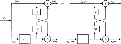
A well-studied problem in digital signal processing (e.g., Haykin, 1991), is the linear prediction problem, in which the structure of the predictor is fixed ahead of time to be a linear transformation of the data. The “forward” linear prediction problem is to predict a future value of a stationary discrete-time random sequence {y(k), k = 1, 2,…} using a set of past samples of the sequence. Let ![]() denote the predicted value of y(k) that uses M past measurements; i.e.,
denote the predicted value of y(k) that uses M past measurements; i.e.,
(16-35)
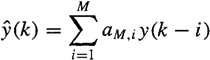
The forward prediction error filter (PEF) coefficients, aM,1,…aM,M, are chosen so that either the mean-squared or least-squares forward prediction error (FPE), fM(k), is minimized, where
(16-36)
![]()
Note that in this filter design problem the length of the filter, M, is treated as a design variable, which is why the PEF coefficients are argumented by M. Note, also, that the PEF coefficients do not depend on tk; i.e., the PEF is a constant coefficent predictor. We will see, in Lessons 17, that our state predictor and filter are time-varying digital filters.
Predictor ![]() uses a finite window of past measurements: y(k – 1), y(k – 2),…, y(k – M). This window of measurements is different for different values of tk. This use of the measurements is quite different than our use of the measurements in state prediction, filtering, and smoothing. The latter are based on an expanding memory, whereas the former is based on a fixed memory (see Lesson 3).
uses a finite window of past measurements: y(k – 1), y(k – 2),…, y(k – M). This window of measurements is different for different values of tk. This use of the measurements is quite different than our use of the measurements in state prediction, filtering, and smoothing. The latter are based on an expanding memory, whereas the former is based on a fixed memory (see Lesson 3).
We return to the minimization of ![]() in Lessons 19.
in Lessons 19.
Digital signal-processing specialists have invented a related type of linear prediction named backward linear prediction in which the objective is to predict a past value of a stationary discrete-time random sequence using a set of future values of the sequence. Of course, backward linear prediction is not prediction at all; it is smoothing (interpolation). But the term backward linear prediction is firmly entrenched in the DSP literature.
Let ![]() denote the predicted value of y(k – M) that uses M future measurements; i.e.,
denote the predicted value of y(k – M) that uses M future measurements; i.e.,

The backward PEF coefficients CM, 1,…, CM,M are chosen so that either the mean-squared or least-squares backward prediction error (BPE), bM(k), is minimized, where
(16-38)
![]()
Both the forward and backward PEFs have a filter architecture associated with them that is known as a tapped delay line (Figure 16-2). Remarkably, when the two filter design problems are considered simultaneously, their solutions can be shown to be coupled. This is the main reason for introducing the backward prediction error filter design problem. Coupling occurs between the forward and backward prediction errors. For example, if the forward and backward PEF coefficients are chosen to minimize ![]() , respectively, then we can show that the following two equations are true:
, respectively, then we can show that the following two equations are true:
(16-39)
![]()
(16-40)
![]()
where m = 1,2,…, M, k = 1,2,…, and coefficent Γ m is called a reflection coefficient. The forward and backward PEF coefficients can be calculated from the reflection coefficients.
Figure 16-2 Tapped delay line architecture for the forward prediction error filter. A similar structure exists for the backward prediction error filter.
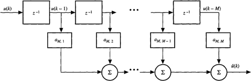
Figure 16-3 Lattice prediction error filter of order M.
A block diagram for (16-39) and (16-40) is depicted in Figure 16-3. The resulting filter architecture is called a lattice. Observe that the lattice filter is doubly recursive in both time, k, and filter order, m. The tapped delay line is only recursive in time. Changing its filter length leads to a completely new set of filter coefficients. Adding another stage to the lattice filter does not affect the earlier reflection coefficients. Consequently, the lattice filter is a very powerful architecture.
No such lattice architecture is known for mean-squared state estimators. The derivation of the lattice architecture depends to a large extent on the assumption that the process to be “predicted” is stationary. Our state-variable model is almost always associated with a nonstationary process. Lesson 19 treats the very special case where the state vector becomes stationary.
Summary Questions
1. The proper initial conditions for state estimation are:
(a) ![]() = 0 and P(0|0) = Px(0)
= 0 and P(0|0) = Px(0)
(b) ![]() = mx(0) and P(-l|0) = 0
= mx(0) and P(-l|0) = 0
(c) ![]() = mx(0) and P(0|0) = Px(0)
= mx(0) and P(0|0) = Px(0)
2. The statement P(k + l|k) = Px(k + 1) is:
(a) always true
(b) never true
(c) obvious
3. Prediction is possible only because we have:
(a) measurements
(b) a known measurement model
(c) a known state equation model
4. If ![]() is an innovations process, then:
is an innovations process, then:
(a) it is white
(b) ![]() is also an innovations process
is also an innovations process
(c) it is numerically the same as z(k + 1)
5. The single-stage predictor is:
(a) ![]()
(b) ![]()
(c) ![]()
6. If u(k) = 0 for all k, then ![]() , where j < k, equals:
, where j < k, equals:
(a) Φ (k,j)![]()
(b) ![]()
(c) Φ(j,k)![]()
7. In forward linear prediction, we:
(a) predict a past value of a stationary discrete-time random sequence using a past set of measurements
(b) predict a future value of a stationary discrete-time random sequence using a past set of measurements
(c) predict a future value of a stationary discrete-time random sequence using a future set of measurements
8. Which of the following distinguish the forward linear predictor from our state predictor?
(a) its length is treated as a design variable
(b) it is a linear transformation of innovations
(c) it uses a finite window of measurements, whereas the state predictor uses an expanding memory
(d) it is noncausal
(e) its coefficients don’t depend on time
9. Two architectures associated with linear prediction are:
(a) tapped delay line
(b) pi-network
(c) lattice
(d) systolic array
(e) neural network
Problems
16-1. Develop the counterpart to Theorem 16-1 for the case when input u(k) is random and independent of Z(j). What happens if u(k) is random and dependent on Z(j)?
16-2. For the innovations process ![]() , prove that
, prove that ![]() when i < j.
when i < j.
16-3. In the proof of part (b) of Theorem 16-2, we make repeated use of the orthogonality principle, stated in Corollary 13-3. In the latter corollary f′[Z(k)] appears to be a function of all the measurements used in ![]() . In the expression
. In the expression ![]() certainly is not a function of all the measurements used in
certainly is not a function of all the measurements used in ![]() . What is f[.] when we apply the orthogonality principle to
. What is f[.] when we apply the orthogonality principle to ![]() , i > j, to conclude that this expectation is zero?
, i > j, to conclude that this expectation is zero?
16-4. Refer to Problem 15-7. Assume that u(k) can be measured [e.g., u(k) might be the output of a random number generator] and that a = a[z(l), z(2),…, z(k – 1)]. What is ![]() ?
?
16-5. Consider the following autoregressive model: z(k + n) = a1z(k + n – 1) – a2z(k + n – 2) –… – anz(k) + w(k + n) in which w(k) is white noise. Measurements z(k), z(k + 1),…, z(k + n – 1) are available.
(a) Compute ![]() .
.
(b) Explain why the result in part (a) is the overall mean-squared prediction of z(k + n) even if w(k + n) is non-Gaussian.
16-6. The state vector covariance matrix can be determined from (see Lesson 15)
![]()
whereas the single-stage predicted state estimation error covariance can be determined from
![]()
The similarity of these equations has led many a student to conclude that Px(k) = ![]() . Explain why this is incorrect.
. Explain why this is incorrect.
16-7. (Keith M. Chugg, Fall 1991) In this lesson we developed the framework for mean-squared predicted state estimates for the basic state-variable model. Develop the corresponding framework for the MAP estimator [i.e., the counterparts to Equations (16-4) and (16-11)].
16-8. (Andrew David Norte, Fall 1991) We are given n measurements z(l), z(2),…, z(n) that are zero mean and jointly Gaussian. Consequently, the innovations is a linear combination of these measurements; i.e.,
(16-8.1)
![]()
(a) Express (16-8.1) in vector-matrix form as ![]() .
.
(b) Demonstrate, by an explicit calculation, that ![]() .
.
(c) Given the three measurements z(l), z(2), and z(3) and their associated covariance matrix
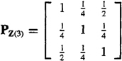
find the numerical elements of matrix Γ that relate the innovations to the measurements.
(d) Using the results obtained in part (c), find the numerical values of the innovations covariance matrix ![]() .
.
(e) Show that Z(3) can be obtained from ![]() , thereby showing that Z(3) and
, thereby showing that Z(3) and ![]() are causally invertible.
are causally invertible.
16-9. (Gregg Isara and Loan Bui, Fall 1991) Curly, Moe, and Larry have just been hired by the Department of Secret Military Products to monitor measurements of the test setup shown in Figure P16-9.
Figure P16-9
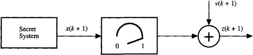
A set of measurements had been recorded earlier with the dial setting of the gain box set to unity. Curly, Moe, and Larry are to monitor a second set of measurements to verify the first. Since the supervisor left no instructions regarding the gain box setting, Curly decides it should be 1/3 because there are 3 people monitoring the measurements. Now
x(k + 1) = 0.5x(k) + 1.25w(k)
and the measurement equations are
zf(k + 1) = x(k + 1) + v(k + 1)
and
zs(k + 1) = 0.333x(k + 1) + v(k + 1)
where zf(k + 1) and zs(k + 1) correspond to the first and second sets of measurements, respectively.
(a) Compute and compare ![]() (l|0) for the two sets of measurements, assuming
(l|0) for the two sets of measurements, assuming ![]() = 0.99 for both systems.
= 0.99 for both systems.
(b) Given that ![]() =
= ![]() (l|0) + K(l)
(l|0) + K(l)![]() (l|0) and K(l)=P(l|0)h[hP(l|0)h+r]-1, find the equations for
(l|0) and K(l)=P(l|0)h[hP(l|0)h+r]-1, find the equations for![]() (2|l) for the two sets of measurements assuming that P(0|0) = 0.2, q = 10, and r = 5.
(2|l) for the two sets of measurements assuming that P(0|0) = 0.2, q = 10, and r = 5.
(c) For zf(1) = 0.8 and z s(l) = ![]() zf(1), compare the predicted estimates
zf(1), compare the predicted estimates![]() f(2|1) and
f(2|1) and![]() s(2|1)
s(2|1)
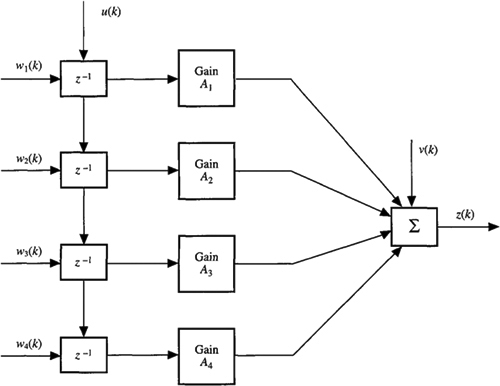
16-10.(Todd A. Parker and Mark A. Ranta, Fall 1991) Using single-stage prediction techniques, design a tool that could be used to estimate the output of the FIR system depicted in Figure PI6-10. Note that u(k) is the system input, which is deterministic, Wi (k) are Gaussian white noise sequences representing errors with the register delay circuitry (i.e., the z-1, and v(k) is a Gaussian white measurement noise sequence. What is the error covariance of the predicted output value?
Figure P16-10
16-11.(Gregory Caso, Fall 1991) For the ARmodel suggested in Problem 16-5, determine the mean-squared p-step predictor ![]() where
where ![]() when the measurements
when the measurements ![]() are available.
are available.