Lesson D
Introduction to State-variable Models and Methods

Summary

State-variable models are widely used in controls, communications, and signal processing. This lesson provides a brief introduction to such models. To begin, it explains the notions of state, state variables, and state space. This culminates in what is meant by a state-variable model, a set of equations that describes the unique relations among a system’s input, output, and state.

Many state-variable representations can result in the same input/output system behavior. We obtain a number of important and useful state-variable representations for single-input, single-output, discrete, linear time-invariant systems, including moving average, autoregressive, and autoregressive moving average.

What can we do with a state-variable model? We can compute a system’s output, given its inputs and initial conditions. A closed-form formula is obtained for doing this. We can also determine the system’s transfer function in terms of the matrices that appear in the state-variable model.

Because a linear time-invariant system can be described in many equivalent ways, including a state-variable model or a transfer function model, it is important to relate the properties of these two representations. We do this at the end of this lesson.

When you complete this lesson, you will be able to (1) express a linear time-invariant system in state-variable format; (2) understand the equivalence of difference equation and state-variable representations; (3) compute the solution to a state-variable model; (4) evaluate the transfer function of a state-variable model; and (5) understand the connections between a state-variable model and a transfer function model.

Notions of State, State Variables, and State Space

The state of a dynamic system (the material in this lesson is taken from Mendel, 1983, pp. 26–41 and 14–16) at time t = t₀ is the amount of information at t₀ that, together with the inputs defined for all values of t ≥ t₀, determines uniquely the behavior of the system for all t ≥ t₀. For systems of interest to us, the state can be represented by a column vector x called the state vector, whose dimension is n × 1.

When the system input is real valued and x is finite dimensional, our state space, defined as an n-dimensional space in which x₁(t), x₂(t),…, x_n(t) are coordinates, is a finite-dimensional real vector space. The state at time t of our system will be defined by n equations and can be represented as a point in n-dimensional state space.

EXAMPLE D-1

The following second-order differential equation models many real devices:

(D-1)

The solution to this differential equation requires two initial conditions in addition to knowledge of input ω(t) for t ≥ t₀. Any two initial conditions will do, although x(t₀) and x(t₀) are most often specified. We can choose x(t) = col[x₁(t), x₂(t)] = col[x(t), (t)] as our 2 × 1 state vector. The state space is two dimensional and is easily visualized as in Figure D-1. Observe how x(t_i) is represented as a point in the two-dimensional state space. When we connect all these points together, we obtain the trajectory of the system in state space.

Figure D-1 Trajectories in two-dimensional state space for (a) overdamped and (b) underdamped systems. (After J. M. Mendel et al. (1981), Geophysics, 46, 1399.)

Visualization is easy in two- and three-dimensional state spaces. In higher-dimensional spaces, it is no longer possible to depict the trajectory of the system, but it is possible to abstract the notions of a point and trajectory in such spaces.

By a state-variable model we mean the set of equations that describes the unique relations among the input, output, and state. It is composed of a state equation and an output equation. A continuous-time state-variable model is

(D-2)

(D-3)

State equation (D-2) governs the behavior of the state vector x(t) (x for short); it is a vector first-order differential equation. Output equation (D-3) relates the outputs to the state vector and inputs. In (D-2) and (D-3), x(t) is an n × 1 state vector, u(t) is an r × 1 control input vector, and y(t) is an m × 1 observation vector; A is, an n × n state transition matrix, B and D are n × r and m × r input distribution matrices, respectively (they distribute the elements of u into the proper state and output equations), and C is an m × n observation matrix.

It is possible to have two distinctly different types of inputs acting on a system: controlled and uncontrolled inputs. A controlled input is either known ahead of time (e.g., a sinusoidal function with known amplitude, frequency, and phase) or can be measured (e.g., the output of a random number generator). An uncontrolled input cannot be measured (e.g., a gust of wind acting on an airplane). Usually, an uncontrolled input is referred to as a disturbance input. Such inputs are included in our basic state-variable model. Here we assume that our state-variable model includes only controlled inputs.

EXAMPLE D-2

Here we demonstrate how to express the second-order model stated in Example D-l in state-variable format. To begin, we normalize (D-l) by making the coefficient of the second derivative unity:

(D-4)

where and Choosing x₁(t) = x(t) and as our state varibles, we observe that

and

These two state equations can be expressed [as in (D-2)] as

Here x(t) = col[x₁(t), x₂(t)],

and u(t) is a scalar input u(t).

To complete the description of the second-order differential equation as a state-variable model, we need an output equation. If displacement is recorded, then y₁(t) = x(t), which can be expressed in terms of state vector x(t) as

On the other hand, if velocity is recorded, then .

Observe that there is no direct transmission of input u(t) into these measurements; hence, D = 0 for both y₁(t) and y₂(t). The same is not true if acceleration is recorded, for in that case

Finally, if two or more signals can be measured simultaneously, then the measurements can be collected (as in (D-3)) as a vector of measurements. For example, if x(t) and can both be recorded, then

A state-variable model can also be defined for discrete-time systems using a similar notion of state vector. Indeed, discrete-time state-variable models are now more popular than continuous-time models because of their applicability to digital computer systems and digital filtering. In many applications it is therefore necessary to convert a continuous-time physical system into an equivalent discrete-time model. Among many discretization methods, one direct approach is to transform a differential equation into a compatible difference equation. See, also, Lessons 23.

EXAMPLE D-3

We discretize the second-order differential equation in Example D-l by letting

and

Making the appropriate substitutions, we obtain

where c₁ = cδ – 2m, k₁ = kδ² – cδ + m, and m₁ = mδ². A commonly used discretization of time is t = nδ; it is also common to use a normalized time unit, achieved by setting δ = 1. The preceding equation can then be further simplified to

a second-order difference equation. For other ways to approximate and , see Taylor and Antoniotti (1993).

In the next section we shall demonstrate how a state-variable model for a difference equation is easily derived. Here we note that a discrete-time state-variable model is again composed of a state equation and an output equation:

(D-5)

(D-6)

State equation (D-5) is a vector first-order difference equation. Equations (D-5) and (D-6) are usually defined for k = 0, 1,…. When y(0) is not physically available or is undefined, it is customary to express the output equation as

(D-6’)

Equations (D-5) and (D-6’) then constitute our state- variable model for k = 0, 1,…. Quantities x(k), u(k), y(k), Φ, Ψ, D, and H have the same definitions as given above for the continuous-time state-variable model.

So as to see the forest from the trees, all our remaining discussions are limited to single-input, single-output linear time-invariant systems. The more general case is treated in the main body of Lessons 15, in the section The Basic State-variable Model.

Constructing State-variable Representations

Many state-variable representations can result in the same input/output system behavior. In this section we obtain a number of important and useful state-variable representations for single-input, single-output (SISO) discrete, linear time-invariant (LTI) systems. Derivations are by means of examples; then general results are stated.

How we obtain a state-variable model depends on our starting point. There are four possibilities: we may be given (1) a collection of differential or difference equations, obtained as in Example D-l from physical principles, (2) a transfer function, (3) an impulse response function, or (4) impulse response data. We shall discuss case 2 in detail. Case 1 has been illustrated in Example D-l. Case 3 can be reduced to case 4 simply by sampling the impulse response function. Case 4 is related to the field of approximation and is beyond the scope of this book.

Our objective is to find state-variable representations for LTI SISO discrete-time systems. We wish to represent such systems by a pair of equations of the form

(D-7)

(D-8)

We must learn not only how to choose the state vector x, but also how to specify the elements of the matrices that appear in the state-variable model in terms of the parameters that appear in the transfer function models.

All-zero (Moving Average) Models

EXAMPLE D-4

The MA model

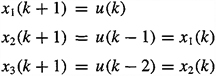
(D-9)

is easily converted to a third-order state-variable model by choosing state variables x₁, x₂, and x₃ as follows: x₁(k) = u(k – 1), x₂(k) = u(k – 2), and x₃(k) = u(k – 3). Equation (D-9), which is treated as an output equation [i.e., Equation (D-8)], is reexpressed in terms of x₁, x₂, and x₃ as

(D-10)

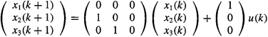
To obtain the associated state equation, we observe that

(D-11)

These three equations are grouped in vector-matrix form to give

(D-12)

Additionally, y(k) can be written as

(D-13)

Equations (D-12) and (D-13) constitute the state-variable representation of the MA model in (D-9).

If y(k) also contains the term β₀u(k), we proceed exactly as before, obtaining state equation (D-12). In this case, observation equation (D-13) is modified to

(D-14)

The term β₀u(k) acts as a direct throughput of input u(k) into the observation.

Using this example, we observe that a state-variable representation for the discrete-time MA model

(D-15)

is

(D-16)

(D-17)

Quantities Φ, Ψ, h′, and d are indicated in (D-16) and (D-17).

All-pole (Autoregressive) Models

EXAMPLE D-5

The discrete-time AR model

(D-18)

associated with the transfer function

(D-19)

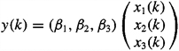
is easily converted to a third-order state-variable model by choosing state variables x₁, x², and x₃ as follows: x₁(k) = y(k), x₂(k) = y(k + 1), and x₃(k) = y(k + 2). Then

or

(D-20)

Additionally, because y(k) = x₁(k)

(D-21)

Equations (D-20) and (D-21) constitute the state-variable representation for the AR model (D-18).

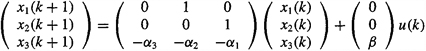
More generally, for the discrete-time AR transfer function

(D-22)

which implies the AR difference equation

(D-23)

(D-24)

qualifies as a state vector. The AR system is described in state variable form as

(D-25)

(D-26)

Pole-Zero (Autoregressive Moving Average) Models

The literature on linear systems contains many state-variable models for pole-zero models [Chen, 1984, and Kailath, 1980, for example]. In this section we describe a few of them.

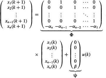
The controllable canonical form state-variable representation for the discrete-time ARMA model

(D-27)

which implies the ARMA difference equation

(D-28)

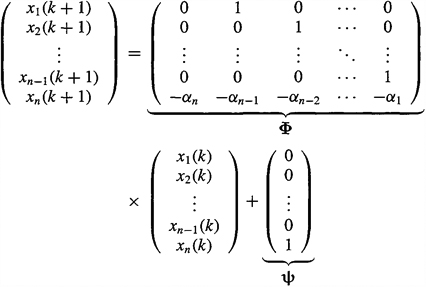
is

(D-29)

and

(D-30)

A very nice feature of this representation is that the α and β coefficients from the difference equation appear unaltered in (D-29) and (D-30). The same cannot be said about all state-variable representations.

EXAMPLE D-6

Rather than prove this result in general, we illustrate the proof for the case when n = 3, for which the third-order ARMA model is

(D-31)

The associated transfer function is

(D-32)

Introduce intermediate variable y₁(k) whose z transform is Y₁(Z):

(D-33)

Doing this is equivalent to treating the ARMA transfer function H(z) as a cascade of two transfer functions; i.e., H(z) = Y(z)/U(z) = H₁(z)H₂(z), where H₁(z) = Y_l(z)/U(z) = 1/(z³ + α₁z² + α₂z + α₃) and H₂(z) = Y(z)/Y₁(z) = β₁z² + β₂z + β₃. Equate the numerator and denominator terms of (D-33) to see that where

(D-34)

and

(D-35)

Equation (D-35) is an autoregressive model, and (D-34) relates intermediate variable y₁(k) y(k)

Using results from Example (D-5), we choose x₁(k) = y₁(k), x₂(k) = y₁(k + 1), and x₃(k) = y₁(k + 2); hence, (D-34) and (D-35) can be expressed as

(D-36)

and

(D-37)

where x(k) = col(x₁(k), x₂(k), x₃(k)). The results in (D-36) and (D-37) are precisely those obtained by setting n = 3 in (D-29) and (D-30).

A completely different state-variable model is obtained when we begin by expanding the transfer function of the system into a partial fraction expansion.

EXAMPLE D-7

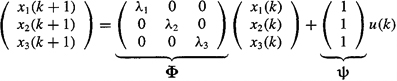
Here we express H(z), given in (D-32), as a sum of three terms:

(D-38)

where λ₁, λ₂, and λ₃, the poles of H(z), are the roots of the characteristic equation z³ + α₁z² + α₂z + α₃ = 0. For the purposes of this example, we assume that λ₁, λ₂ and λ₃ are real and unequal. Equation (D-38) constitutes the partial fraction expansion of H(z).

We now view y(k) as the sum of the outputs from three systems that are in parallel (see Figure D-2). Consider the input/output equation for y₁(k),

Figure D-2 Parallel connection of three first-order systems.

(D-39)

Let x₁(k) = y₁(k) so that (D-39) can be written in terms of state variable x₁(k) as

(D-40)

Proceeding similarly for y₂(k) and y₃(k), letting x₂(k) = y₂(k) and x₃(k) = y₃(k), we find that

(D-41)

and

(D-42)

Combining (D-40) – (D-42), we obtain our final state-variable model:

(D-43)

where

(D-44)

In this state-variable model, matrix Φ is diagonal, which is useful in some computations. If λ₁ is complex, then λ₂ = λ₁*, and Φ and h will contain complex numbers. We explain how to handle this situation in Example D-8. Finally, if two or more of the poles are equal, the structure of Φ will be different, because the structure of the partial fraction expansion is not that given in (D-38).

The approach to developing a state-variable model illustrated by this example leads to a representation known as the Jordan canonical form. We do not state its structure for an arbitrary transfer function. It can be obtained for any AR or ARMA model by the following procedure: (1) calculate the poles of the system; (2) perform a partial fraction expansion; (3) for real (single or repeated) poles, treat each term in the partial fraction expansion as a single-input, single-output (SISO) system and obtain its state-variable representation (as in Example D-7); (4) for complex poles, treat the conjugate pole pairs together as a second-order system and obtain a state-variable representation for it that involves only real numbers; and (5) combine the representations obtained in steps 3 and 4 in the output equation.

EXAMPLE D-8

Here we give a very useful state-variable model for a subsystem composed of two complex conjugate poles:

(D-45)

This transfer function is associated with the second-order difference equation

(D-46)

which can be expressed in state-variable form as

(D-47)

where

(D-48)

We leave the verification of this representation to the reader.

Many other equivalent state-variable models are possible for ARMA systems. The equivalence of different state-variable models is demonstrated later under Miscellaneous Properties.

Solutions of State Equations for Time-invariant Systems

Now that we know how to construct state-variable models, what can we do with them? In this section we show how to obtain y(k) given u(k) and initial conditions x(0). We also show how easy it is to obtain an expression for the transfer function Y(z)/U(z) from a state-variable model.

State equation (D-7) is recursive and, as we demonstrate next, easily solved for x(k) as an explicit function of x(0), u(0), u(1),…, and u(k – 1). Once we know x(k), it is easy to solve for y(k), because y(k) = h′x(k) (we assume d = 0 here).

To solve (D-7) for x(k), we proceed as follows:

etc.

By this iterative procedure we see that a pattern has emerged for expressing x(k) as a function of x(0), u(0), u(1),…, u(k – 1); i.e.,

(D-49)

where k = 1, 2,…. An inductive proof of (D-49) is found in Mendel (1973, pp. 21-23).

Assuming that y(k) = h′x(k), we see that

(D-50)

The first term on the right-hand side of (D-50) is owing to the initial conditions; it is the transient (homogeneous) response. The second term is owing to the forcing function u; it is the forced response and is a convolution summation.

Equation (D-49) provides us with directions for going from an initial state x(0) directly to state x(k). For linear systems we can also reach x(k) by first going from x(0) to state x(j) and then going from x(y) to x(k). In fact, x(k) can be expressed in terms of x(j) as

(D-51)

where k ≥ j + 1.

Matrix Φ^k-i in (D-49)-(D-51) is called a state transition matrix for the homogeneous system x(k + 1) = Φx(k). We denote this matrix Φ(k, i). It has the following properties:

(D-52)

a. Identity property:

(D-53)

b. Semigroup property:

(D-54)

c. Inverse property:

Proofs of these properties use the definition of Φ(k, i) and are left to the reader. The semigroup property was already used when we showed that x(k) could be reached from x(0) by going from x(0) to x(j) and then from x(j) to x(k).

Next we direct our attention to computing the transfer function Y(z)/U(z).

EXAMPLE D-9

Consider a second-order ARMA model written in controllable canonical form as

(D-55)

(D-56)

To compute Y(z)/U(z), we must express X₁(z) and X₂(z) as functions of U(z), after which it is easy to express Y(z) as a function of U(z), using (D-56).

Take the z-transform of the two state equations (D-55), to show that

Treat these equations as a system of two equations in the two unknowns X₁(z) and X₂(Z), and rewrite them as

or

(D-57)

Recognize that (D-57) can also be written, symbolically, as

(D-58)

in which I is the 2 X 2 identity matrix and X(Z) is the Z-transfrom of x(k) [i.e., X_i(Z) = Z{x₁(k)},i = 1, 2].

This example demonstrates that we can take the z-transform of state equation (D-7) without having to do it equation by equation.

Proceeding formally to determine Y(z)/U(z), we first take the z-transform of state equation (D-7)

(D-59)

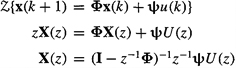
Finally, we combine (D-59) and (D-60) to give us the desired transfer function.

Then we take the Z-transfrom of the output equation y(k) = h′x(k)

(D-60)

or

Finally, we combine (D-59) and (D-60) to give us the desired transfer function

(D-61)

We denote this transfer function as H(z) to remind us of the well-known fact (Chen, 1984) that the transfer function is the z-transform of the unit spike (impulse) response of the system h(k). Observe that we have just determined the transfer function for a LTI SISO discrete-time system in terms of the parameters Φ, Ψ, and h of a state-variable representation of that system.

Matrix (I – z^–1 Ψ)^–1, which appears in H(z), has the power-series expansion

(D-62)

Hence,

(D-63)

Denoting the coefficients of H(z) as h(j), we see that

(D-64)

These coefficients are commonly known as Markov parameters.

Equation (D-64) is important and can be used in two ways: (1) Given (Φ, Ψ, h), compute the sampled impulse response {h(1), h(2),…}, and (2) given {h(1), h(2),…}, compute (Φ, Ψ, h).

Miscellaneous Properties

In this section we present some important facts about stability, nonuniqueness, and flexibility of state-variable models.

Recall that the asymptotic stability of a LTI SISO discrete-time system is guaranteed if all the poles of H(z) lie inside the unit circle in the complex z domain. For H(z) = N(z)/D(z), we know that the poles of H(z) are the roots of D(z). We also know that

(D-65)

where Q(z) is an n × n matrix whose elements are simple polynomials in z whose degree is at most n – 1, and det(zI – Φ), the characteristic polynomial of Φ, is a scalar nth-degree polynomial. The poles of H(z) are therefore the roots of the characteristic polynomial of Φ

Recall from matrix theory [Franklin, 1968, for example] that ≠ 0 is called an eigenvector of matrix Φ if there is a scalar λ such that

(D-66)

In this equation λ is called an eigenvalue of Φ corresponding to . Equation (D-66) can be written as

Because ≠ 0, by definition of an eigenvector, matrix (λI – Φ) must be singular; hence,

(D-68)

We see, therefore, that the eigenvalues of Φ are the roots of det (λI – Φ), the characteristic polynomial of Φ. By means of this line of reasoning, we have demonstrated the truth of:

Property 1. The poles of H(z) are the eigenvalues of matrix Φ.

The asymptotic stability of a LTI SISO discrete-time system is therefore guaranteed if all the eigenvalues of Φ lie inside the unit circle.

Next we direct our attention to the nonuniqueness and flexibility of state-variable representations. We know that many state-variable representations are possible for the same LTI SISO system, for example, the controllable and Jordan canonical forms for ARMA systems. One form may be better for numerical calculations, whereas a different form may be better for parameter estimation, and so on. Regardless of the form used, we must be sure that from an input/output point of view there are no theoretical differences (numerical differences may occur owing to word length and computer roundoff).

Suppose we make a change (transformation) of state variables, as follows:

(D-69)

where P is a constant nonsingular n × n matrix. Then

(D-70)

(D-71)

can be expressed in terms of z(k) as

(D-72)

(D-73)

We shall show that the x system in (D-70) and (D-71) and the z system in (D-72) and (D-73) are equivalent from an input/output point of view. First we show that P^–1 ΦP has the same eigenvalues as Φ. Then we show that H(z) is the same for both systems.

Property 2. The eigenvalues of ΦP^–1ΦP are those of Φ.

Proof. Let and M are said to be similar matrices. Let and P_M(Z) = det(zI – M). Consequently,

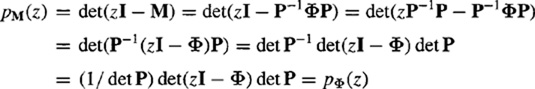
where we have used the following well-known facts about determinants: (1) the determinant of a product of matrices equals the product of the determinants of the matrices that comprise the product matrix, and (2) the determinant of a matrix inverse equals 1 divided by the determinant of the matrix.

Property 3. Let H_x (z) and H_z(z) denote Y(z)/U(z) for the x system in (D-70) and (D-71) and the z system in (D-72) and (D-73), respectively. Then

(D-74)

Proof. From (D-61),

(D-75)

Repeating the analysis that led to H_x(z), but for (D-72) and (D-73), we find that

(D-76)

Consequently,

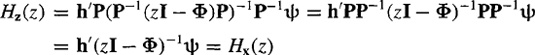
To arrive at this result, we have used the fact, from matrix theory, that (GHL)_–1 = L_-1H_-1G_-1.

Computation

See the discussion on computation in Lessons 15.

Summary Questions

1. A state-variable model:

(a) must be linear and time invariant

(b) occurs in the frequency domain

(c) is composed of a state equation and an output equation

2. Matrix Φ(t, τ) satisfies a linear:

(a) time-varying matrix differential equation

(b) time-invariant matrix differential equation

(c) time-varying matrix difference equation

3. An nth-order difference equation can be expressed as a vector first-order state equation with:

(a) n + m states, where m equals the number of measurements

(b) exactly n states

(c) less than n states

4. In a state-variable model, the choice of state variables is:

(a) unique

(b) done by solving an optimization problem

(c) not unique

5. The Jordan canonical form has a plant matrix that is:

(a) block diagonal

(b) always diagonal

(c) full

6. The semigroup property of state transition matrix Φ means that we can:

(a) stop at x(j) and return to starting point x(i)

(b) stop at x(j) and continue to x(i)

(c) return to starting point x(k) after having reached x(i)

7. The z-transform of a state equation:

(a) must be taken equation by equation

(b) does not exist

(c) does not have to be taken equation by equation

8. The poles of the system’s transfer function are the:

(a) eigenvalues of matrix Φ^–1

(b) eigenvalues of matrix Φ

(c) roots of det (zI – ψψ′)

9. For a linear transformation of state variables, i.e., z(k) = P^–1(k)x(k), which of the following are true?

(a) the z system’s eigenvalues are scaled versions of the x system’s eigenvalues

(b) the eigenvalues of P^-1ΦP are those of Φ

(c) if the x system is minimum phase, then the z system is nonminimum phase

(d) the transfer function remains unchanged

(e) if the x system is minimum phase, then the z system is minimum phase

Problems

D-l. Verify the state-variable model given in Example D-8 when a subsystem has a pair of complex conjugate poles.

D-2. Prove the truth of the identity property, semigroup property, and inverse property, given in (D-52), (D-53) and (D-54), respectively, for the state transition matrix. Provide a physical explanation for each of these important properties.

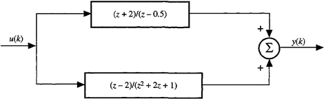
D-3. Determine a state-variable model for the system depicted in Figure PD-3.

Figure PD-3.

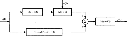
D-4. Determine a state-variable model for the system depicted in Figure PD-4.

Figure PD-4.

D-5. Determine a state-variable model for the system depicted in Figure PD-5.

Figure PD-5.

D-6. Determine a state-variable model for the system depicted in Figure PD-6.

Figure PD-6.

D-7. Determine a state-variable model for the system depicted in Figure PD-7.

Figure PD-7.

D-8. Depicted in Figure PD-8 is the interconnection of recording equipment, coloring filter, and band-pass filter to a channel model. Noise v(k) could be additive measurement noise or could be used to model digitization effects associated with a digital band-pass filter. Assume that the four subsystems are described by the following state vectors: S₁: x₁(n₁ × 1); S2: x₂(n₂ × 1); S₃: x₃(n₃ × 1); and S₄: x₄(n₄ × 1); Obtain a state-variable model for this system that is of dimension n1 + n2 + n3 + n4.

Figure PD-8.

D-9. Determine the eigenvalues of the system in:

(a) Problem D-3

(b) Problem D-4

(c) Problem D-5

(d) Problem D-6

(e) Problem D-7

D-10. (Computational Problem) For the system in Figure PD-4, compute y(k) in two different ways for 25 time units, one of which must be by solution of the system’s state equation. Sketch the results.

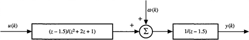
D-ll. Consider the system depicted in Figure PD-11. Note that a pole-zero cancellation occurs as a result of the cascade of the two subsystems. Explain whether or not this is a stable system.

Figure PD-11.