Lesson 3
Least-squares Estimation: Batch Processing
Summary
The main purpose of this lesson is the derivation of the classical batch formula of (weighted) least squares. The term batch means that all measurements are collected together and processed simultaneously. A second purpose of this lesson is to demonstrate that least-squares estimates may change in numerical value under changes of scale. One way around this difficulty is to use normalized data.
Least-squares estimates require no assumptions about the nature of the generic linear model. Consequently, the formula for the least-squares estimator (LSE) is easy to derive. We will learn in Lesson 8, that the price paid for ease in derivation is difficulty in performance evaluation.
The supplementary material at the end of this lesson contrasts least squares, total least squares, and constrained total least squares. The latter techniques are frequently more powerful than least squares, especially in signal-processing applications.
When you complete this lesson you will be able to (1) derive and use the classical batch formulas of (weighted) least squares; these are theoretical formulas that should not be programmed as is for digital computation; numerically well behaved linear algebra programs are commercially available for computational purposes; (2) explain the sensitivity of (weighted) least squares to scale change; and (3) explain the difference between least squares, total least squares, and constrained total least squares.
Introduction
The method of least squares dates back to Karl Gauss around 1795 and is the cornerstone for most estimation theory, both classical and modern. It was invented by Gauss at a time when he was interested in predicting the motion of planets and comets using telescopic measurements. The motions of these bodies can be completely characterized by six parameters. The estimation problem that Gauss considered was one of inferring the values of these parameters from the measurement data.
We shall study least-squares estimation from two points of view: the classical batch-processing approach, in which all the measurements are processed together at one time, and the more modern recursive processing approach, in which measurements are processed only a few (or even one) at a time. The recursive approach has been motivated by today’s high-speed digital computers; however, as we shall see, the recursive algorithms are outgrowths of the batch algorithms.
The starting point for the method of least squares is the linear model
(3-1)
![]()
where Z(k) = col (z(k), z(k – 1),…, z(k – N + 1)), z(k) = h′ (k)θ + v(k), and the estimation model for Z(k) is
(3-2)
![]()
We denote the (weighted) least-squares estimator of θ as [![]() ]
]![]() . In this lesson and the next two we shall determine explicit structures for this estimator.
. In this lesson and the next two we shall determine explicit structures for this estimator.
Gauss: A Short Biography
Carl Friederich Gauss was born on April 30, 1777, in Braunschweig, Germany. Although his father wanted him to go into a trade, his mother had the wisdom to recognize Gauss’s genius, which manifested itself at a very early age, and saw to it that he was properly schooled.
E.T. Bell (1937), in his famous essay on Gauss, refers to him as the “Prince of Mathematicians.” Courant (1969) states that “Gauss was one of the three most famous mathematicians in history, in company with Archimedes and Newton.”
Gauss invented the method of least squares at the age of 18. This work was the beginning of a lifelong interest in the theory of observation. He attended the University of Göttingen from October 1795 to September 1798. Some say that these three years were his most prolific. He received his doctor’s degree in absentia from the University of Helmstedt in 1799. His doctoral dissertation was the first proof of the fundamental theorem of algebra.
In 1801 he published his first masterpiece, Arithmetical Researches, which revolutionized all of arithmetic and established number theory as an organic branch of mathematics. In 1809 he published his second masterpiece, Theory of the Motion of Heavenly Bodies Revolving Round the Sun in Conic Sections, in which he predicted the orbit of Ceres. E.T. Bell felt that Gauss’s excursions into astronomical works was a waste of 20 years, during which time he could have been doing more pure mathematics. This is an interesting point of view (not shared by Courant); for what we take as very important to us in estimation theory, least squares and its applications, has been viewed by some mathematicians as a diversion.
In 1812 Gauss published another great work on the hypergeometric series from which developed many applications to differential equations in the nineteenth century. Gauss invented the electric telegraph (working with Wilhelm Weber) in 1833. He made major contributions in geodesy, the theories of surfaces, conformal mapping, mathematical physics (particularly electromagnetism, terrestrial magnetism, and the theory of attraction according to Newtonian law), analysis situs, and the geometry associated with functions of a complex variable.
Gauss was basically a loner. He published his results only when they were absolutely polished, which made his publications extremely difficult to understand, since so many of the details had been stripped away. He kept a diary throughout his lifetime in which he briefly recorded all of his “gems.” This diary did not become known until many years after his death. It established his precedence for results associated with the names of many other famous mathematicians (e.g., he is now credited with being one of the founders of non-Euclidean geometry). For discussions of an interesting feud between Gauss and Legendre over priority to the method of least squares, see Sorenson (1970).
Gauss died at 78 on February 23, 1855. As Bell says, “He lives everywhere in mathematics.”
Number of Measurements
Suppose that θ contains n parameters and Z(k) contains N measurements. If N < n, we have fewer measurements than unknowns and (3-1) is an underdetermined system of equations that does not lead to unique values for θ1, θ2,…, θn. If N = n, we have exactly as many measurements as unknowns, and as long as the n measurements are linearly independent, so that H–1 (k) exists, we can solve (3-1) for θ as
(3-3)
![]()
Because we cannot measure V(k), it is usually neglected in the calculation of (3-3). For small amounts of noise this may not be a bad thing to do, but for even moderate amounts of noise this will be quite bad. Finally, if N > n, we have more measurements than unknowns, so (3-1) is an overdetermined system of equations. The extra measurements can be used to offset the effects of the noise; i.e., they let us “filter” the data. Only this last case is of real interest to us. Some discussions on the underdetermined case are given in Lesson 4.
Objective Function and Problem Statement
A direct approach for obtaining ![]() is to choose it so as to minimize the sum of the squared errors between its components and the respective components of θ, i.e., to minimize
is to choose it so as to minimize the sum of the squared errors between its components and the respective components of θ, i.e., to minimize
The solution to this minimization problem is ![]() = θ which, of course is a useless result, because, if we knew θ ahead of time, we would not need to estimate it.
= θ which, of course is a useless result, because, if we knew θ ahead of time, we would not need to estimate it.
A less direct approach for obtaining ![]() is based on minimizing the objective function
is based on minimizing the objective function
(3-4)
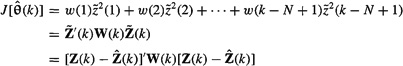
where
(3-5)
![]()
and weighting matrix W(k) must be symmetric and positive definite, for reasons explained later.
No general rules exist for how to choose W(k). The most common choice is a diagonal matrix such as
![]()
When |μ| < 1 so that 1/μ > 1, recent errors (and associated measurements) [![]() ] are weighted more heavily than past ones [
] are weighted more heavily than past ones [![]() ]. Such a choice for W(k) provides the weighted least-squares estimator with an “aging” or “forgetting” factor. When |μ| > 1, recent errors are weighted less heavily than past ones. Finally, if μ = 1, so that W(k) = I, then all errors are weighted by the same amount. When W(k) = I,
]. Such a choice for W(k) provides the weighted least-squares estimator with an “aging” or “forgetting” factor. When |μ| > 1, recent errors are weighted less heavily than past ones. Finally, if μ = 1, so that W(k) = I, then all errors are weighted by the same amount. When W(k) = I, ![]() , whereas for all other W(k),
, whereas for all other W(k), ![]() Note also that if W(k) = cI, where c is a constant, then
Note also that if W(k) = cI, where c is a constant, then ![]() (see Problem 3-2).
(see Problem 3-2).
Our objective is to determine the ![]() that minimizes
that minimizes ![]() .
.
Derivation of Estimator
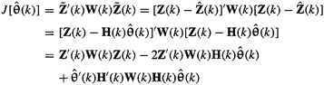
To begin, we express (3-4) as an explicit function of ![]() , using (3-2):
, using (3-2):
(3-6)
Next, we take the vector derivative of ![]() with respect to
with respect to ![]() , but before doing this recall from vector calculus, that:
, but before doing this recall from vector calculus, that:
If m and b are two n x 1 nonzero vectors, and A is an n x n symmetric matrix, then
(3-7)
![]()
and
(3-8)
![]()
Using these formulas, we find that
(3-9)
![]()
Setting ![]() , we obtain the following formula for
, we obtain the following formula for ![]() :
:
(3-10)
![]()
Note, also, that
(3-11)
![]()
By substituting (3-10) into (3-6), we obtain the minimum value of ![]() :
:
(3-12)
![]()
Comments
1. Matrix H’(k)W(k)H(k) must be nonsingular for its inverse to exist. Matrix H’(k)W(k)H(k) is said to be nonsingular if it has an inverse satisfying
![]()
If W(k) is positive definite, then it can be written uniquely as W(k) = L’(k)L(k), where L(k) is a lower triangular matrix with positive diagonal elements. Consequently, we can express H’(k)W(k)H(k) as
![]()
If A (k) has linearly independent columns, i.e., is of maximum rank, then A′(k)A(k) is nonsingular. Finally, rank [L(k)H(k)] = rank[H(k)], because L(k) is nonsingular. Consequently, if H(k) is of maximum rank, then A′(k)A(k) is nonsingular, so [A′(k)A(k)]–1 = [H′(k)W(k)H(k)]–1 exists. The two conditions that have fallen out of this analysis are that W(k) must be positive definite and H(k) must be of maximum rank.
2. How do we know that ![]() minimizes
minimizes ![]() We compute
We compute ![]() and see if it is positive definite [which is the vector calculus analog of the scalar calculus requirement that
and see if it is positive definite [which is the vector calculus analog of the scalar calculus requirement that ![]() minimizes
minimizes ![]() and
and ![]() is positive]. Doing this, we see that
is positive]. Doing this, we see that
![]()
because H′(k)W(k)H(k) is invertible.
3. Estimator ![]() processes the measurements Z(k) linearly; thus, it is referred to as a linear estimator. It processes the data contained in H(k) in a very complicated and nonlinear manner.
processes the measurements Z(k) linearly; thus, it is referred to as a linear estimator. It processes the data contained in H(k) in a very complicated and nonlinear manner.
4. When (3-9) is set equal to zero, we obtain the following system of normal equations:
(3-13)
![]()
This is a system of n linear equations in the n components of ![]() .
.
In practice, we do not compute ![]() using (3-10), because computing the inverse of H′(k)W(k)H(k) is fraught with numerical difficulties. Instead, the normal equations are solved using stable algorithms from numerical linear algebra. Golub and Van Loan (1989) have an excellent chapter, entitled “Orthogonalization and Least Squares Methods,” devoted to numerically sound ways for computing
using (3-10), because computing the inverse of H′(k)W(k)H(k) is fraught with numerical difficulties. Instead, the normal equations are solved using stable algorithms from numerical linear algebra. Golub and Van Loan (1989) have an excellent chapter, entitled “Orthogonalization and Least Squares Methods,” devoted to numerically sound ways for computing ![]() from (3-13) (see, also, Stewart, 1973; Bierman, 1977; and Dongarra, et al., 1979). They state that “One tactic for solution [of (3-13)] is to convert the original least squares problem into an equivalent, easy-to-solve problem using orthogonal transformations. Algorithms of this type based on Householder and Givens transformations… compute the factorization H′(k)W(k)H(k) = Q(k)t)R(k), where Q(k) is orthogonal and R(k) is upper triangular.”
from (3-13) (see, also, Stewart, 1973; Bierman, 1977; and Dongarra, et al., 1979). They state that “One tactic for solution [of (3-13)] is to convert the original least squares problem into an equivalent, easy-to-solve problem using orthogonal transformations. Algorithms of this type based on Householder and Givens transformations… compute the factorization H′(k)W(k)H(k) = Q(k)t)R(k), where Q(k) is orthogonal and R(k) is upper triangular.”
In Lesson 4 we describe how (3-10) can be computed using the very powerful singular-value decomposition (SVD) method. SVD can be used for both the overdetermined and underdetermined situations.
Based on this discussion, we must view (3-10) as a useful”theoretical” formula and not as a useful computational formula.
5. Using the fact that ![]() equation (3-13) can also be reexpressed as
equation (3-13) can also be reexpressed as
(3-14)
![]()
which can be viewed as an orthogonality condition between ![]() and W(k)H(k). Orthogonality conditions play an important role in estimation theory. We shall see many more examples of such conditions throughout this book. For a very lucid discussion on the least-squares orthogonality principle, see Therrien (1992, pp. 525-528). See, also, Problems 3-12 and 3-13.
and W(k)H(k). Orthogonality conditions play an important role in estimation theory. We shall see many more examples of such conditions throughout this book. For a very lucid discussion on the least-squares orthogonality principle, see Therrien (1992, pp. 525-528). See, also, Problems 3-12 and 3-13.
6. Estimates obtained from (3-10) will be random! This is because Z(k) is random, and in some applications even H(k) is random. It is therefore instructive to view (3-10) as a complicated transformation of vectors or matrices of random variables into the vector of random variables ![]() In later lessons, when we examine the properties of
In later lessons, when we examine the properties of ![]() , these will be statistical properties because of the random nature of
, these will be statistical properties because of the random nature of ![]() .
.
7. The assumption that θ is deterministic was never made during our derivation of ![]() ; hence, (3-10) and (3-11) also apply to the estimation of random parameters. We return to this important point in Lesson 13. If θ is random, then a performance analysis of
; hence, (3-10) and (3-11) also apply to the estimation of random parameters. We return to this important point in Lesson 13. If θ is random, then a performance analysis of ![]() is much more difficult than when θ is deterministic. See Lesson 8 for some performance analyses of
is much more difficult than when θ is deterministic. See Lesson 8 for some performance analyses of ![]() .
.
EXAMPLE 3-1 (Mendel, 1973, pp. 86–87)
Suppose we wish to calibrate an instrument by making a series of uncorrelated measurements on a constant quantity. Denoting the constant quantity as θ, our measurement equation becomes
(3-15)
![]()
where k = 1, 2,…, N. Collecting these N measurements, we have
(3-16)

Clearly, H = col (1, 1,…, 1); henced
(3-17)
![]()
which is the sample mean of the N measurements. We see, therefore, that the sample mean is a least-squares estimator.![]()
EXAMPLE 3-2 (Mendel, 1973)
Figure 3-1 depicts simplified third-order pitch-plane dynamics for a typical, high-performance, aerodynamically controlled aerospace vehicle. Cross-coupling and body-bending effects are neglected. Normal acceleration control is considered with feedback on normal acceleration and angle-of-attack rate. Stefani (1967) shows that if the system gains are chosen as
Figure 3-1 Pitch-plane dynamics and nomenclature: Ni, input normal acceleration along the negative Z axis; KNi gain on Ni; δ, control-surface deflection; Mδ, control-surface effectiveness; ![]() rigid-body acceleration; α, angle of attack; Mα, aerodynamic moment effectiveness; Kα, control gain on α; Zα, normal acceleration force coefficient; μ, axial velocity; Nα, system-achieved normal acceleration along the negative Z axis; KNa, control gain on Na (reprinted from Mendel, 1973, p. 33, by courtesy of Marcel Dekker, Inc.).
rigid-body acceleration; α, angle of attack; Mα, aerodynamic moment effectiveness; Kα, control gain on α; Zα, normal acceleration force coefficient; μ, axial velocity; Nα, system-achieved normal acceleration along the negative Z axis; KNa, control gain on Na (reprinted from Mendel, 1973, p. 33, by courtesy of Marcel Dekker, Inc.).

(3-18)
![]()
(3-19)

and
(3-20)
![]()
then
(3-21)
![]()
Stefani assumes Zα 1845/μ is relatively small, and chooses C1 = 1400 and C2 = 14, 000. The closed-loop response resembles that of a second-order system with a bandwidth of 2 Hz and a damping ratio of 0.6 that responds to a step command of input acceleration with zero steady-state error.
In general, Mα, Mδ, and Zα are dynamic parameters and all vary through a large range of values. Also, Mα may be positive (unstable vehicle) or negative (stable vehicle). System response must remain the same for all values of Mα, Mδ and Zα; thus, it is necessary to estimate these parameters so that KNi, Ka, and KNa can be adapted to keep C1 and C2 invariant at their designed values. For present purposes we shall assume that Mα, Mδ, and Zα are frozen at specific values.
From Figure 3-1,
(3-22)
![]()
and
(3-23)
![]()
Our attention is directed at the estimation of Mα and Mδ in (3-22). We leave it as an exercise for the reader to explore the estimation of Zα in (3-23).
Our approach will be to estimate Mα and Mδ from the equation
(3-24)
![]()
where ![]() denotes the measured value of
denotes the measured value of ![]() that is corrupted by measurement noise
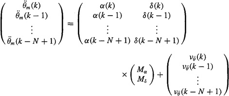
that is corrupted by measurement noise ![]() . We shall assume (somewhat unrealistically) that α(k) and δ(k) can both be measured perfectly. The concatenated measurement equation for N measurements is
. We shall assume (somewhat unrealistically) that α(k) and δ(k) can both be measured perfectly. The concatenated measurement equation for N measurements is
(3-25)
Hence, the least-squares estimates of Mα and Mδ are
(3-26)

Fixed and Expanding Memory Estimators
Estimator ![]() uses the measurements z(k – N + 1), z(k – N + 2),…, z(k). When N is fixed ahead of time,
uses the measurements z(k – N + 1), z(k – N + 2),…, z(k). When N is fixed ahead of time, ![]() uses a fixed window of measurements, a window of length N, and
uses a fixed window of measurements, a window of length N, and ![]() is then referred to as a fixed-memory estimator. The batch weighted least-squares estimator, obtained in this lesson, has a fixed memory.
is then referred to as a fixed-memory estimator. The batch weighted least-squares estimator, obtained in this lesson, has a fixed memory.
A second approach for choosing N is to set it equal to k; then ![]() uses the measurements z(l), z(2),…, z(k). In this case,
uses the measurements z(l), z(2),…, z(k). In this case, ![]() uses an expanding window of measurements, a window of length k, and
uses an expanding window of measurements, a window of length k, and ![]() is then referred to as an expanding-memory estimator. The recursive weighted least-squares estimator, obtained in Lesson 5, has an expanding memory.
is then referred to as an expanding-memory estimator. The recursive weighted least-squares estimator, obtained in Lesson 5, has an expanding memory.
Scale Changes and Normalization of Data
Least-squares (LS) estimates may not be invariant under changes of scale. One way to circumvent this difficulty is to use normalized data.
As long as the elements of Z(k), the z(k – j)’s (j = 0, 1,…, N – 1), are scalars, there is no problem with changes in scale. For example, if measurements of velocity are in miles per hour or are scaled to feet per second, we obtain the same weighted least-squares or unweighted least-squares estimates. Reasons for this are explored in Problems 3-7 and 3-8. If, on the other hand, the elements of Z(k), the z(k – j)’s (j = 0, 1,…, N – 1), are vectors (see the section in Lesson 5 entitled “Generalization to Vector Measurements”), then scaling of measurements can be a serious problem, as we now demonstrate.
Assume that observers A and B are observing a process; but observer A reads the measurements in one set of units and B in another. Let M be a diagonal matrix of scale factors relating A to B; ZA(k) and ZB(k) denote the total measurement vectors of A and B, respectively. Then
(3-27)
![]()
which means that
(3-28)
![]()
Let ![]() and
and ![]() denote the WLSEs associated with observers A and B, respectively, where
denote the WLSEs associated with observers A and B, respectively, where ![]() and
and ![]() or
or
(3-29)
![]()
It seems a bit peculiar though to have different weighting matrices for the two WLSEs. In fact, if we begin with ![]() then it is impossible to obtain
then it is impossible to obtain ![]() such that
such that![]() . The reason for this is simple. To obtain
. The reason for this is simple. To obtain ![]() , we set WA(k) = I, in which case (3-29) reduces to WB(k) = (M–1)2 ≠ I.
, we set WA(k) = I, in which case (3-29) reduces to WB(k) = (M–1)2 ≠ I.
Next, let NA and NB denote diagonal normalization matrices for ZA(k) and ZB(k), respectively. We shall assume that our data is always normalized to the same set of numbers, i.e., that
(3-30)
![]()
Observe that
(3-31)
![]()
and
(3-32)
![]()
From (3-30), (3-31), and (3-32), we see that
(3-33)
![]()
We now find that
(3-34)
![]()
and
(3-35)
![]()
Substituting (3-33) into (3-35), we then find
(3-36)
![]()
Comparing (3-36) and (3-34), we conclude that ![]() if WB(k) = WA(k). This is precisely the result we were looking for. It means that, under proper normalization,
if WB(k) = WA(k). This is precisely the result we were looking for. It means that, under proper normalization, ![]() and, as a special case,
and, as a special case, ![]() .
.
One way to normalize data is to divide all values by the maximum value of the data. Another way is to work with percentage values, since a percentage value is a ratio of numerator to denominator quantities that have the same units; hence, percentage value is unitless.
Computation
See Lesson 4 for how to compute ![]() or
or ![]() using the singular-value decomposition and the pseudoinverse.
using the singular-value decomposition and the pseudoinverse.
Total least squares estimates, which are described in the Supplementary Material at the end of this lesson, can be computed using the following M-file in Hi-Spec:
tls: Total least squares solution to an overdetermined system of linear equations.
Supplementary Material Least Squares, Total Least Squares, and Constrained Total Least Squares
Consider the overdetermined linear system of equations
(3-37)
![]()
which must be solved for x. Numerical linear algebra specialists (e.g., Stewart, 1973, and Golub and Van Loan, 1989) provide the following very interesting interpretation for the least-squares solution to (3-37). Suppose there are “errors” associated with the numbers that are entered into the vector b, i.e., b → b + Δ b, in which case (3-37) actually is
(3-38)
![]()
This equation can now be expressed as our generic linear model, as
(3-39)
![]()
Here b, A, x, and –Δb play the roles of Z(k), H(k), θ, and V(k), respectively. In our derivation of the least-squares estimator, we minimized ![]() , which, in the notation of (3-39) means that we minimized [b – Ax]′[b – Ax] = Δb′Δb; i.e., the least-squares solution of (3-38) finds the x that minimizes the errors in the vector b.
, which, in the notation of (3-39) means that we minimized [b – Ax]′[b – Ax] = Δb′Δb; i.e., the least-squares solution of (3-38) finds the x that minimizes the errors in the vector b.
Many signal-processing problems lead to a linear system of equations like (3-37). In these problems the elements of b must first be estimated directly from the data; e.g., they could be autocorrelations, cross-correlations, higher-order statistics, etc. As such, the estimated statistics are themselves in error; hence, in these problems there usually is an error associated with b. Unfortunately, in these same problems there usually are also errors associated with the numbers entered into matrix A (see Problem 2-8). These elements may also be autocorrelations or higher-order statistics; hence, in many signal-processing problems (3-37) actually becomes
(3-40)
![]()
Solving for x using least squares ignores the errors in A.
Equation (3-40) can be reexpressed as
(3-41)
![]()
Golub and Van Loan (1980, 1989) determined a solution x of (3-41) that minimizes the Frobenius norm of (ΔA|Δb). [Note that the Frobenius norm of the real L x P matrix M is defined by
They called this the “total least squares (TLS)” solution, XTLS. Their solution involves the singular-value decomposition of (ΔA|Δb). Van Huffel and Vandewalle (1991) provide a comprehensive treatise on TLS.
One major assumption made in TLS is that the errors in A are independent, as are the errors in b; i.e., the elements of ΔA, ΔAij are totally independent, as are the elements of Δb, Δbi. Unfortunately, this is not the situation in most signal-processing problems, where matrix A has a specific structure (e.g., Toeplitz, block Toeplitz, Hankel, block Hankel, and circulant). Additionally, b may also contain elements that also appear in A. Consequently, the errors ΔA and Δb are not usually independent in signal-processing applications. Yet, TLS is widely used in such applications and often (if not always) gives much better results than does least squares. Apparently, doing something to account for errors in both A and b is better than only accounting for errors in b.
Abatzoglou, Mendel, and Harada (1991) developed a variation of TLS that is appropriate for the just described situation in which elements of ΔA and Δb are dependent. The dependency can be represented as linear constraints among the elements of ΔA and Δb. They determine a solution x to (3-41) that in essence minimizes a norm of (ΔA|Δb) subject to linear constraints between the elements of ΔA and Δb. They called this the “constrained total least squares (CTLS)” solution XCTLS. Their solution requires mathematical programming; hence, it is computationally more intensive than the TLS solution; but examples demonstrate that it outperforms TLS.
When the signal-to-noise ratio is high, it is frequently true that elements of ΔA and Δb are very small, in which case XLS, XTLS, and XCTLS give essentially the same results. When the signal-to-noise ratio is low so that elements of ΔA and Δb are large, there will be a significant payoff when using TLS or CTLS.
Summary Questions
1. The method of least squares is credited to:
(a) Lagrange
(b) Rayleigh
(c) Gauss
2. A weighted least-squares estimator reduces to a least-squares estimator when:
(a) past measurements are weighted more heavily than present measurements
(b) past measurements are weighted the same as present measurements
(c) past measurements are weighted less heavily than present measurements
3. The normal equations:
(a) should be programmed for solution using a matrix inversion routine
(b) should be solved using Gaussian elimination
(c) should be solved using stable algorithms from numerical linear algebra that use orthogonal transformations
4. When N is set equal to k, then ![]() is known as a:
is known as a:
(a) fixed-memory estimator
(b) expanding-memory estimator
5. Least-squares estimates may not be invariant under scale change. One way to circumvent this difficulty is to use:
(a) normalized data
(b) squared data
(c) redundant data
6. Let NA and NB denote symmetric normalization matrices for ZA(k) and ZB(k), respectively. The condition that our data are always normalized to the same set of numbers is:
(a) NA ZA(k) = NB ZB(k)
(b) ZA (k)NB = NA ZB (k)
(c) ZA(k)NA = NB ZB(k)
7. Weighted least-squares estimates are:
(a) deterministic
(b) random
(c) a mixture of deterministic and random
8. Gauss was worried that his discovery of the method of least squares would be credited to:
(a) Laplace
(b) Legendre
(c) Lagrange
9. Consider the equation Ax = b. Which of the following statements are true?
(a) least-squares is associated with accounting for the errors in A, that is, ΔA
(b) least-squares is associated with accounting for the errors in b, that is, Δb
(c) TLS accounts for errors in both A and b, but it assumes all elements of ΔA are independent, as are all elements of Δb
(d) TLS accounts for errors in both A and b, but it assumes some elements of ΔA are dependent, as are some elements of Δb
(e) CTLS accounts for errors in both A and b, and it assumes elements of ΔA are nonlinearly related, as are some elements of Δb
(f) CTLS accounts for errors in both A and b, and it assumes elements of ΔA are linearly related, as are some elements of Δb
(g) TLS solution XTLS can be obtained using singular-value decomposition
Problems
3-1. Derive the formula for ![]() by completing the square on the right-hand side of the expression for
by completing the square on the right-hand side of the expression for ![]() in (3-6). In the calculus approach to deriving
in (3-6). In the calculus approach to deriving ![]() , described in the text, invertibility of H′(k)W(k)H(k) is needed in order to solve (3-9) for
, described in the text, invertibility of H′(k)W(k)H(k) is needed in order to solve (3-9) for ![]() . Is this condition still needed in this problem’s algebraic derivation? If so, how does it occur in the algebraic derivation of
. Is this condition still needed in this problem’s algebraic derivation? If so, how does it occur in the algebraic derivation of ![]() ? What is the main advantage of the algebraic derivation over the calculus derivation?
? What is the main advantage of the algebraic derivation over the calculus derivation?
3-2. In the text we stated that ![]() is obtained when the weighting matrix is chosen as W(k) = I. More generally,
is obtained when the weighting matrix is chosen as W(k) = I. More generally, ![]() is obtained when the weighting matrix is chosen as W(k) = cI, where c is a constant. Verify the truth of this statement. What happens to J
is obtained when the weighting matrix is chosen as W(k) = cI, where c is a constant. Verify the truth of this statement. What happens to J![]() in (3-12), and is it important?
in (3-12), and is it important?
3-3. (Prof. G. B. Giannakis) Show that weighted least squares can be interpreted as least squares applied to filtered versions of Z(k) and H(k). [Hint: Decompose W(k) as W(k) = L′(k)D(k)L(k), where L(k) is lower triangular and D(k) is diagonal.] What is the “filter”? What happens if W(k) is itself diagonal?
3-4. Here we explore the estimation of Z∞ in (3-23). Assume that N noisy measurements of Na (k) are available, i.e., ![]() . What is the formula for the least-squares estimator of Zα?
. What is the formula for the least-squares estimator of Zα?
3-5. Here we explore the simultaneous estimation of Mα, Mδ, and Zα in (3-22) and (3-23). Assume that N noisy measurements of ![]() are available, i.e.,
are available, i.e.,![]() Determine the least-squares estimator of Mα, Mδ, and Zα. Is this estimator different from
Determine the least-squares estimator of Mα, Mδ, and Zα. Is this estimator different from ![]() and
and ![]() obtained just from
obtained just from ![]() measurements and
measurements and ![]() obtained just from
obtained just from ![]() measurements?
measurements?
3-6. In a curve-fitting problem we wish to fit a given set of data z(l), z(2),…, z(N) by the approximating function (see, also, Example 2-3)
![]()
where φj (k) (j = 1, 2,…, n) are a set of prespecified basis functions.
(a) Obtain a formula for ![]() that is valid for any set of basis functions.
that is valid for any set of basis functions.
(b) The simplest approximating function to a set of data is the straight line. In this case, ![]() , which is known as the least-squares or regression line. Obtain closed-form formulas for
, which is known as the least-squares or regression line. Obtain closed-form formulas for ![]() .
.
3-7. Suppose z(k) = θl + θ2k, where z(1) = 3 miles per hour and z(2) = 7 miles per hour. Determine ![]() based on these two measurements. Next, redo these calculations by scaling z(1) and z(2) to the units of feet per second. Are the least-squares estimates obtained from these two calculations the same? Use the results developed in the section entitled “Scale Changes and Normalization of Data” to explain what has happened here.
based on these two measurements. Next, redo these calculations by scaling z(1) and z(2) to the units of feet per second. Are the least-squares estimates obtained from these two calculations the same? Use the results developed in the section entitled “Scale Changes and Normalization of Data” to explain what has happened here.
3-8. (a) Under what conditions on scaling matrix M is scale invariance preserved for a least-squares estimator?
(b) If our original model is nonlinear in the measurements [e.g., z(k) = θz2 (k - 1) + v(k)], can anything be done to obtain invariant WLSEs under scaling?
3-9. (Tony Hung-yao Wu, Spring 1992) Sometimes we need to fit data that are exponential in nature. This requires the approximating function to be of the form y = beax. An easy way to fit this model to data is to work with the logarithm of the model, i.e., ln y = In b + ax. Obtain least-squares estimates for a and b for the following data:
i |
x(i) |
y(i) |
i |
1.00 |
5.10 |
2 |
1.25 |
5.79 |
3 |
1.50 |
6.53 |
4 |
1.75 |
7.45 |
5 |
2.00 |
8.46 |
3-10. (Ryuji Maeda, Spring 1992) In an experiment to determine Planck's constant h using the photoelectric effect, the following linear relationship is obtained between retarding potential V and frequency of the incident light v:
![]()
where e is the charge of an electron (assume its value is known), nv is the measurement noise associated with measuring V, and hv0 is the work function.
(a) The following measurements are made: V1,…, VN, and v1,…, VN. Derive the formula for ![]() .
.
(b) Suppose the following data have been obtained from an experiment in which sodium is used as the “target”: V0 = 4.4 x 10¹⁴ Hz and e = 1.6 x 10⁻¹⁹.
v x 10-14 (Hz) |
V (V) |
6.9 |
1.1 |
9.0 |
1.8 |
12.1 |
3.1 |
Find the numerical value of ![]() for these data.
for these data.
3-11. (Liang-Jin Lin, Spring 1992) Supose that Y is modeled as a quadratic function of X, i.e.,
Y(X) = aX2 + bX + c
and the measurements of Y, denoted Z, are subject to measurement errors.
(a) Given a set of measurements {X(i), Z(i)}, i = 1,2,…,N, determine a formula for col ![]() .
.
(b) Calculate col ![]() for the following data. (Note: The actual values of parameters a, b, and c used to generate these data are 0.5, 1.5, and 3, respectively.)
for the following data. (Note: The actual values of parameters a, b, and c used to generate these data are 0.5, 1.5, and 3, respectively.)
![]()
3-12. Let H(k) be expressed as H(k) = (h1(k)|h2(k)|… |hn(k)).
(a) Show that, for least-squares estimates,
![]()
(b) Explain why ![]() lies in the subspace defined by the n vectors h1(k), h2 (k),…, hn(k).
lies in the subspace defined by the n vectors h1(k), h2 (k),…, hn(k).
(c) Does Z(k) lie in ![]() ’s subspace?
’s subspace?
(d) Provide a three-dimensional diagram to clarify parts (b) and (c) for n = 2.
(e) Explain why ![]() is the orthogonal projection of z(k) onto the subspace spanned by the hi(k)’s. Use your diagram from part (d) to do this.
is the orthogonal projection of z(k) onto the subspace spanned by the hi(k)’s. Use your diagram from part (d) to do this.
(f) How do the results from parts (a)-(e) assist your understanding of least-squares estimation?
3-13. The derivation of the least-squares estimator makes extensive use of the approximation of Z(k) as ![]() = H(k)
= H(k)![]() .
.
(a) Show that ![]() can be expressed as
can be expressed as ![]() = PH(k) (k)Z(k), where the matrix PH(k)(k) is called a projection matrix. Why is PH(k)(k) called a projection matrix? (Hint: See Problem 3-12.)
= PH(k) (k)Z(k), where the matrix PH(k)(k) is called a projection matrix. Why is PH(k)(k) called a projection matrix? (Hint: See Problem 3-12.)
(b) Prove that PH(k)(k) is an idempotent matrix.
(c) Showthat ![]() Matrix
Matrix ![]() is associated with the complementary (orthogonal) subspace to H(k) (see Problem 3-12). Prove that
is associated with the complementary (orthogonal) subspace to H(k) (see Problem 3-12). Prove that ![]() is also idempotent.
is also idempotent.
(d) Prove that ![]()
(e) How do the results from parts (a) - (d) further assist your understanding of least-squares estimation?
3-14. Consider the generic model in (2-1) subject to the restrictions (constraints) Cθ = r, where C is a J x n matrix of known constants and is of rank J, and r is a vector of known constants. This is known as the restricted least-squares problem (Fomby et al., 1984). Let ![]() denote the restricted least-squares estimator of θ. Show that
denote the restricted least-squares estimator of θ. Show that
![]()
(Hint: Use the method of Lagrange multipliers.)