Lesson 9
Best Linear Unbiased Estimation

Summary

The main purpose of this lesson is to develop our second estimator. It is both unbiased and efficient by design and is a linear function of the measurements Z(k). It is called a best linear unbiased estimator (BLUE).

As in the derivation of the WLSE, we begin with our generic linear model; but now we make two assumptions about this model: (1) H(k) must be deterministic, and (2) V(k) must be zero mean with positive definite known covariance matrix R(k). The derivation of the BLUE is more complicated than the derivation of the WLSE because of the design constraints; however, its performance analysis is much easier because we build good performance into its design.

A very remarkable connection exists between the BLUE and WLSE: the BLUE of θ is the special case of the WLSE of θ when W(k) = R^–1 (k). Consequently, all results obtained in Lessons 3, 4, and 5 for can be applied to by setting W(k) = R^–1(k).

In recursive WLSs, matrix P(k) has no special meaning. In recursive BLUE, matrix P(k) turns out to be the covariance matrix for the error between θ and . Recall that in Lesson 3 we showed that weighted least-squares estimates may change in numerical value under changes in scale. BLUEs are invariant under changes in scale.

The fact that H(k) must be deterministic limits the applicability of BLUEs.

When you complete this lesson you will be able to (1) explain and demonstrate how to design an estimator that processes the measurements linearly and has built into it the desirable properties of unbiasedness and efficiency; (2) connect this linear estimator (i.e., the BLUE) with the WLSE; (3) explain why the BLUE is insensitive to scale change; and (4) derive and use recursive BLUE algorithms.

Introduction

Least-squares estimation, as described in Lessons 3, 4, and 5, is for the linear model

(9-1)

where θ is a deterministic, but unknown vector of parameters, H(k) can be deterministic or random, and we do not know anything about V(k) ahead of time. By minimizing , where , we determined that is a linear transformation of Z(k), i.e., . After establishing the structure of , we studied its small and large-sample properties. Unfortunately, is not always unbiased or efficient. These properties were not built into during its design.

In this lesson we develop our second estimator. It will be both unbiased and efficient, by design. In addition, we want the estimator to be a linear function of the measurements Z(k). This estimator is called a best linear unbiased estimator (BLUE) or an unbiased minimum-variance estimator (UMVE). To keep notation relatively simple, we will use to denote the BLUE of θ.

As in least squares, we begin with the linear model in (9-1), where θ is deterministic. Now, however, H(k) must be deterministic and V(k) is assumed to be zero mean with positive definite known covariance matrix R(k). An example of such a covariance matrix occurs for white noise. In the case of scalar measurements, z(k), this means that scalar noise v(k) is white, i.e.,

(9-2)

where δ_kj is the Kronecker δ (i.e., δ_kj = 0 for k ≠ j and δkj = 1 for k = j). Thus,

(9-3)

In the case of vector measurements, z(k), this means that vector noise, v(k), is white, i.e.,

(9-4)

Thus,

(9-5)

i.e., R(k) is block diagonal.

Problem Statement and Objective Function

We begin by assuming the following linear structure for :

(9-6)

where, for notational simplicity, we have omitted subscripting F(k) as F_BLU(k). We shall design F(k) such that

a. is an unbiased estimator of θ, and

b. the error variance for each of the n parameters is minimized. In this way, will be unbiased and efficient, by design.

Recall, from Theorem 6-1, that unbiasedness constrains design matrix F(k), such that

(9-7)

Our objective now is to choose the elements of F(k), subject to the constraint of (9-7), in such a way that the error variance for each of the n parameters is minimized.

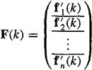
In solving for F_BLU(k), it will be convenient to partition matrix F(k) as

(9-8)

Equation (9-7) can now be expressed in terms of the vector components of F(k). For our purposes, it is easier to work with the transpose of (9-7), H′F′ = I, which can be expressed as

(9-9)

where e_i, is the ith unit vector,

(9-10)

in which the nonzero element occurs in the ith position. Equating respective elements on both sides of (9-9), we find that

(9-11)

Our single unbiasedness constraint on matrix F(k) is now a set of n constraints on the rows of F(k).

Next, we express in terms of f_i(i = 1, 2,…, N). We shall make use of (9-11), (9-1), and the following equivalent representation of (9-6):

(9-12)

Proceeding, we find that

(9-13)

Observe that the error variance for the ith parameter depends only on the ith row of design matrix F(k). We, therefore, establish the following objective function:

(9-14)

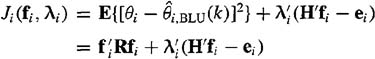
where λ_i, is the ith vector of Lagrange multipliers (see the Supplementary Material at the end of this lesson for an explanation of Lagrange’s method), which is associated with the ith unbiasedness constraint. Observe that the first term in (9-14) is associated with mean-squared error, whereas the second term is associated with unbiasedness. Our objective now is to minimize J_i, with respect to f_i and λ_i (i = 1, 2,…, n).

Why is it permissible to determine f_i and λ_i, for i = 1, 2,…, n by solving n independent optimization problems? Ideally, we want to minimize all J_i,(f_i, λ_i,)’s simultaneously. Consider the following objective function:

(9-15)

Observe from (9-14) that

(9-16)

Clearly, the minimum of J (f₁, f₂,…, f_n, λ₁, λ₂,…, λ_n) with respect to all f₁, f₂,…, f_n, λ₁, λ₂,…,λ_n is obtained by minimizing each J_i,(f_i, λ_i) with respect to each f_i, λ_i. This is because the J_i’s are uncoupled; i.e., J₁ depends only on f₁ and λ₁, J₂ depends only on f₂ and λ₂,…, and J_n depends only on f_n and λ_n.

Derivation of Estimator

A necessary condition for minimizing J_i,(f_i, λ_i,) is ∂, J_i (f_i, λ_i,)/∂f_i = 0(i = 1, 2,…, n); hence,

(9-17)

from which we determine f_i as

(9-18)

For (9-18) to be valid, R^–1 must exist. Any noise V(k) whose covariance matrix R is positive definite qualifies. Of course, if V(k) is white, then R is diagonal (or block diagonal) and R^–1 exists. This may also be true if V(k) is not white. A second necessary condition for minimizing J_i,(f_i, λ_i) is ∂ J_i(f_i, λ_i)/∂λ_i, = 0(i = 1, 2,…, n), which gives us the unbiasedness constraints

(9-19)

To determine λ_i, substitute (9-18) into (9-19). Doing this, we find that

(9-20)

whereupon

(9-21)

(i = 1, 2,…, n). Matrix F(k) is reconstructed from f_i(k), as follows:

(9-22)

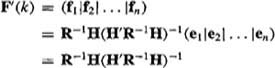
Hence,

(9-23)

which means that

(9-24)

Comparison of and

We are struck by the close similarity between and .

Theorem 9-1. The BLUE of θ is the special case of the WLSE of θ when

(9-25)

W(k) = R^-1(k)

If W(k) is diagonal, then (9-25) requires V(k) to be white.

Proof. Compare the formulas for in (9-24) and in (3-10). If W(k) is a diagonal matrix (which is required in the Lesson 5 derivation of the recursive WLSE), then R(k) is a diagonal matrix only if V(k) is white.

Matrix R^–1(k) weights the contributions of precise measurements heavily and de-emphasizes the contributions of imprecise measurements. The best linear unbiased estimation design technique has led to a weighting matrix that is quite sensible.

Corollary 9-1. All results obtained in Lessons 3, 4, and 5 for can be applied to by setting W(k) = R^–1 (k).

We leave it to the reader to explore the full implications of this important corollary by reexamining the wide range of topics that was discussed in Lessons 3, 4, and 5.

Theorem 9-2 (Gauss-Markov Theorem). If H(k) is deterministic and R(k) = I, then = .

Proof. Using (9-22) and the fact that R(k) = I, we find that

Comparison of and

Why is this a very important result? We have connected two seemingly different estimators, one of which, has the properties of unbiased and minimum variance by design; hence, in this case inherits these properties. Remember though that the derivation of required H(k) to be deterministic.

Some Properties of

To begin, we direct our attention at the covariance matrix of parameter estimation error .

Theorem 9-3. If V(k) is zero mean, then

(9-26)

Proof. We apply Corollary 9-1 to cov[] [given in (8-18)] for the case when H(k) is deterministic, to see that

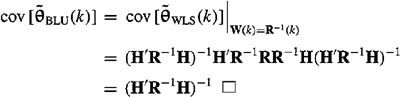
Observe the great simplification of the expression for cov, when . Note, also, that the error variance of given by the ith diagonal element of cov.

Corollary 9-2. When W(k) = R^–1(k), then matrix P(k), which appears in the recursive WLSE of θ equals cov, i.e.,

(9-27)

Proof. Recall Equation (4-13), that

(9-28)

When W(k) = R^–1(k), then

(9-29)

Hence, P(k) = cov because of (9-26).

Soon we will examine a recursive BLUE. Matrix P(k) will have to be calculated, just as it has to be calculated for the recursive WLSE. Every time P(k) is calculated in our recursive BLUE, we obtain a quantitative measure of how well we are estimating θ. Just look at the diagonal elements of P(k), k = 1, 2,…. The same statement cannot be made for the meaning of P(k) in the recursive WLSE. In the recursive WLSE, P(k) has no special meaning.

Next, we examine cov in more detail.

Theorem 9-4. is a most efficient estimator of θ within the class of all unbiased estimators that are linearly related to the measurements Z(k).

In the econometric’s literature (e.g., Fomby et al., 1984) this theorem is known as Aitken’s Theorem (Aitken, 1935).

Proof (Mendel, 1973, pp. 155–156). According to Definition 6-3, we must show that

(9-30)

is positive semidefinite. In (9-30), _a(k) is the error associated with an arbitrary linear unbiased estimate of θ. For convenience, we write Σ as

(9-31)

To compute Σ_a we use the facts that

(9-32)

and

(9-33)

Thus,

(9-34)

Because = F(k)Z(k) and F(k)H(k) = I,

(9-35)

Substituting (9-34) and (9-35) into (9-31) and making repeated use of the unbiasedness constraints H′F′ = H′F′_a = F_aH_a = I, we find that

(9-36)

Making use of the structure of F(k), given in (9-23), we see that Σ can also be written as

(9-37)

Some Properties of

To investigate the definiteness of Σ, consider the definiteness of a′Σa, where a is an arbitrary nonzero vector:

(9-38)

Matrix F (i.e., F_BLU) is unique; therefore, (F_a – F)′a is a nonzero vector, unless F_a – F and a are orthogonal, which is a possibility that cannot be excluded. Because matrix R is positive definite, a′Σa ≥ 0, which means that Σ is positive semidefinite.

These results serve as further confirmation that designing F(k) as we have done, by minimizing only the diagonal elements of cov, is sound.

Theorem 9-4 proves that is most efficient within the class of linear estimators. The cov [] is given in (9-26) as [H′(k)R^–1(k)H(k)]^–1; hence, it must be true that the Fisher information matrix [see (6-45)] for this situation is J(θ) = H′(k)R^–1 (k)H(k). We have been able to obtain the Fisher information matrix in this lesson without knowledge of the probability density function for Z(k), because our BLU estimator has been designed to be of minimum variance within the class of linear estimators.

Next, let us compare our just determined Fisher information matrix with the results in Example 6-4. In that example, J(θ) was obtained for the generic linear model in (9-1) under the assumptions that H(A:) and θ are deterministic and that generic noise V(k) is zero mean multivariate Gaussian with covariance matrix equal to R(k). The latter assumption then lets us determine a probability density function for Z(k), after which we were able to compute the Fisher information matrix, in (6-56), as J(θ) = H′(k)R^–1(k)H(k).

How is it possible that we have arrived at exactly the same Fisher information matrix for these two different situations? The answer is simple. The Fisher information matrix in (6-56) is not dependent on the specific structure of an estimator. It merely provides a lower bound for cov[(k)]. We have shown, in this lesson, that a linear estimator achieves this lower bound. It is conceivable that a nonlinear estimator might also achieve this lower bound; but, because linear processing is computationally simpler than nonlinear processing, there is no need to search for such a nonlinear estimator.

Corollary 9-3. If R(k) = I, then is a most efficient estimator of θ.

The proof of this result is a direct consequence of Theorems 9-2 and 9-4.

Note that we also proved the truth of Corollary 9-3 in Lesson 8 in Theorem 8-3. The proof of Theorem 8-3 is totally within the context of least squares, whereas the proof of Corollary 9-3 is totally within the context of BLUE, which, of course, is linked to least squares by the Gauss-Markov Theorem 9-2.

At the end of Lesson 3 we noted that may not be invariant under scale changes. We demonstrate next that is invariant to such changes.

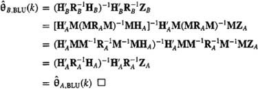
Theorem 9-5. is invariant under changes of scale.

Proof (Mendel, 1973, pp. 156–157). Assume that observers A and B are observing a process; but observer A reads the measurements in one set of units and B in another. Let M be a symmetric matrix of scale factors relating A to B (e.g., 5280 ft/mile, 454 g/lb, etc.), and Z_A(k) and Z_B(k) denote the total measurement vectors of A and B, respectively. Then

(9-39)

which means that

(9-40)

(9-41)

and

(9-42)

Let , and denote the BLUEs associated with observers A and B, respectively; then,

(9-43)

Here is an interesting interpretation of Theorem 9-5. Suppose we “whiten” the data by multiplying Z(k) by R^–1/2(k). Doing this, our generic linear model can be written as

(9-44)

where Z₁(k) = R^–1/2(k)Z(k), H₁(k) = R^–1/2(k)H(k), and V₁(k) = R^–1/2(k)V(k). Note that, when the data are whitened, cov V₁(k) = R₁ = I. If (9-44) is the starting point for BLUE, then

(9-45)

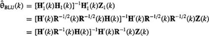
which is precisely the correct formula for . Creating R^–1/2(k)Z(k) properly normalizes the data. This normalization is not actually performed on the data in BLUE. It is performed by the BLUE algorithm automatically.

This suggests that we should choose the normalization matrix N in Lesson 3 as R^–1/2(k); but this can only be done if we know the covariance matrix of V(k), something that was not assumed known for the method of least squares. When R(k) is known and H(k) is deterministic, then use . When R(k) is known and H(k) is not deterministic, use with W(k) = R^–1 (k). We cannot use in the latter case because the BLUE was derived under the assumption that H(k) is deterministic.

Recursive BLUEs

Because of Corollary 9-1, we obtain recursive formulas for the BLUE of θ by setting 1/w(k + 1) = r(k + 1) in the recursive formulas for the WLSEs of θ, which are given in Lesson 5. In the case of a vector of measurements, we set (see Table 5-1) w^–1 (k + 1) = R(k + 1).

Theorem 9-6 (Information form of recursive BLUE). A recursive structure for is

(9-46)

where

(9-47)

and

(9-48)

These equations are initialized by and P^–1 (n) [where P(k) is cov, given in (9-26)] and are used for k = n, n + 1,…, N – 1. These equations can also be used for k = 0, 1,…, N – 1 as long as and P^–1(0) are chosen using Equations (5-21) and (5-20) in Lesson 5, respectively, in which w(0) is replaced by r^–1(0).

Theorem 9-7 (Covariance form of recursive BLUE). Another recursive structure/or is (9-46) in which

(9-49)

and

(9-50)

These equations are initialized by and P(n) and are used for k = n, n + 1,…, N – 1. They can also be used for k = 0, 1,…, N – 1 as long as and P(0) are chosen using Equations (5-21) and (5-20), respectively, in which w(0) is replaced by r^–1(0).

Recall that, in best linear unbiased estimation, . Observe, in Theorem 9-7, that we compute P(k) recursively, and not P^–1(k). This is why the results in Theorem 9-7 (and, subsequently, Theorem 5-2) are referred to as the covariance form of recursive BLUE.

See Problem 9-10 for a generalization of the recursive BLUE to a nondiagonal symmetric covariance matrix.

Computation

Because BLUE is a special case of WLSE, refer to Lessons 4 and 5 for discussions on computation. Of course, we must now set W(k) = R^–1(k) in batch algorithms, or w(k) = 1/r(k) in recursive algorithms.

Supplementary Material: Lagrange’s Method

Lagrange’s method for handling optimization problems with constraints was devised by the great eighteenth century mathematician Joseph Louis Lagrange. In the case of optimizing F(x) subject to the scalar constraint G(x) = g, Lagrange’s method tells us to proceed as follows: form the function

(9-51)

where λ. is a constant, as yet undetermined in value. Treat the elements of x as independent variables, and write down the conditions

(9-52)

Solve these n equations along with the equation of the constraint

(9-53)

to find the values of the n + 1 quantities x₁, x₂,…, x_n, λ. More than one point (x₁, x₂,…, x_n, λ) may be found in this way, but among the points so found will be the points of optimal values of F(x).

Equivalently, form the function

(9-54)

where λ is treated as before. In addition to the n equations ∂J(x, λ)/∂x_i = 0, write down the condition

(9-55)

Solve these n + 1 equations for x and λ.

The parameter λ is called a Lagrange multiplier. Multiple constraints are handled by introducing one Lagrange multiplier for each constraint. So, for example, the vector of n_c constraints G(x) = g is handled in (9-54) by replacing the term λ[G(x) – g] by the term λ′[G(x) – g].

Summary Questions

1. For a BLUE:

(a) H(k) and V(k) must be known

(b) H(k) may be random

(c) H(k) must be deterministic and V(k) may be zero mean

2. = if:

(a) R(k) = W(k)

(b) R(k) = wI

(c) R(k) = I

3. By design, a BLUE is:

(a) consistent and unbiased

(b) efficient and unbiased

(c) a least-squares estimator

4. is invariant under scale changes because:

(a) it was designed to be so

(b) W(k) = R^–1 (k)

(c) R_B(k) = MR_A(k)M

5. The name covariance form of the recursive BLUE (and, subsequently, recursive WLSE) arises, because:

(a) P(k) = cov and we compute P(k) recursively

(b) P(k) = cov and we compute P^–1(k) recursively

(c) P(k) = cov

6. The BLUE of θ is the special case of the WLSE of θ when W(k) equals:

(a) R(k)

(b) R^–1(k)

(c) wI

7. Check off the two design constraints imposed on the BLUE:

(a) is an unbiased estimator of θ

(b) is a linear function of the measurements

(c) the error variance of each of the n parameters is minimized

8. Recursive formulas for the BLUE of θ are obtained from the recursive formulas in Lesson 5 for the WLSE of θ by setting:

(a) w(k + 1) = constant

(b) 1/w(k + 1) = r(k + 1)

(c) w(k + 1) = r(k + 1)

9. When H(k) is random, computations in the derivation of break down in:

(a) the unbiasedness constraint

(b) computing the Lagrange multipliers

(c) computing the error variance

10. When W(k) = R^–1(k), then matrix P(k), which appears in the recursive WLSE of θ, equals:

(a) cov

(b) a diagonal matrix

(c) W(k)

Problems

9-1. (Mendel, 1973, Exercise 3-2, p. 175). Assume H(k) is random and that .

(a) Show that unbiasedness of the estimate is attained when E{F(k)H(k)} = I.

(b) At what point in the derivation of do the computations break down because H(k) is random?

9-2. Here we examine the situation when V(k) is colored noise and how to use a model to compute R(k). Now our linear model is

Z(k + 1) = H(k + 1)θ + v(k + 1)

where v(k) is colored noise modeled as

v(k + 1) = A_vv(k) + ξ(k)

We assume that deterministic matrix A_v is known and that ξ(k) is zero-mean white noise with covariance R_ξ,(k). Working with the measurement difference z^*(k + 1) = z(k + 1) – A_vz(k), write down the formula for in batch form. Be sure to define all concatenated quantities.

9-3. (Sorenson, 1980, Exercise 3-15, p. 130). Suppose and are unbiased estimators of θ with var and var . Let .

(a) Prove that is unbiased.

(b) Assume that and are statistically independent, and find the mean-squared error of .

(c) What choice of α minimizes the mean-squared error?

9-4. (Mendel, 1973, Exercise 3-12, pp. 176–177). A series of measurements z(k) is made, where z(k) = Hθ + v(k), H is an m × n constant matrix, E{v(k)} = 0, and cov[v(k)] = R is a constant matrix.

(a) Using the two formulations of the recursive BLUE, show that (Ho, 1963, pp. 152–154):

(i) P(k + 1)H′ = P(k)H′[HP(k)H′ + R]^–1 R, and

(ii) HP(k) = R[HP(k – 1)H′ + R]^–1HP(k – 1).

(b) Next, show that

(i) P(k)H′ = P(k – 2)H′[2HP(k – 2)H′ + R]^–1R;

(ii) P(k)H′ = P(k – 3)H′[3HP(k – 3)H′ + R]^–1R; and

(iii)P(k)H′ = P(0)H′[kHP(0)H′ + R]^–1R.

(c) Finally, show that the asymptotic form (k → ∞) for the BLUE of θ is (Ho, 1963, pp. 152–154)

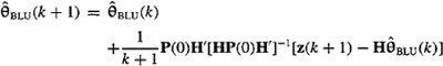
This equation, with its 1/(k + 1) weighting function, represents a form of multidimensional stochastic approximation.

9-5. (Iraj Manocheri, Spring 1992) We are given the BLUE of θ that is based on measurements Z₁(k), where Z₁(k) = H₁(k)θ + V₁(k), E{V₁(k)} = 0, and . Additional measurements Z₂ (k) = H₂(k)θ + V₂ (k), E{V₂ (k)} = 0, and are obtained, where V₂(k) is independent of V₁,(k).

(a) What are the formulas for and ?

(b) Find the batch BLUE of θ given both Z₁,(k) and Z₂ (k).

(c) Find the recursive BLUE of θ given Z₂(k) and .

9-6. (Bruce Rebhan, Spring 1992) One of your colleagues at Major Defense Corporation has come to you with an estimation problem.

(a) Two sets of sensors are used to provide an altitude measurement for the fighter radar you are developing. These sensors have the following covariance (R) matrices associated with their noises:

Your colleague tells you that he plans to take a BLUE estimate of the altitude from each set of sensors. You tell him that you don’t think that’s a good idea. Why not?

(b) Your colleague returns to you, again seeking your sage advice regarding BLUE estimates. This time he has two different sets of sensors with noise covariance matrices

He tells you that neither set of sensors is conducive to a BLUE estimate, since neither covariance matrix is “white.” Do you agree with him?

(c) Your colleague returns once more, this time with covariance matrices associated with another two sets of sensors:

He tells you that since both of the noise covariance matrices are of the form R = he may take BLUEs from both set of sensors. You agree with this much. He then says that, furthermore, since both BLUEs will reduce to the LSE (by the Gauss-Markov theorem), it makes no difference which BLUE is used by the radar processor. You disagree with his conclusion, and tell him to use the BLUE from the sensors associated with R₁. What is your reasoning?

9-7. (Richard S. Lee, Jr., Spring 1992) This computer-oriented problem is designed to explore the differences between the LS and BLU estimators. (a) Generate a set of measurement data, {z(k), k = 0, 1,…, 309}, where

z(k) = a + bk + v(k)

in which a = 1.0 and b = 0.5, v(k) is Gaussian zero-mean white noise with variance r(k), where r(k) = 1.0 for k = 0, 1,…,9, and r(k) is uniformly distributed between 1 and 100 for k = 10, 11,…, 309.

(b) Using the generated measurements [z(k), k = 0, 1,…, 9}, determine and using the batch LS estimator.

(c) For each value of k = 10, 11,…, 309, determine and using the recursive LS algorithm. Use the values of (9) and (9) determined in part (b) to initialize the recursive algorithm. Plot (k) and (k) versus k.

(d) Repeat part (b) using the BLUE. Compare your results to those obtained in part (b).

(e) Repeat part (c) using the BLUE. Compare your results to those obtained in part (c).

9-8. Suppose covariance matrix R is unknown and we decide to estimate it using least squares so that we can then use this estimate in the formula for the BLUE of θ; i.e., we estimate R as

Show that is rank 1 and is therefore singular; consequently, cannot be computed. Note that if R can be suitably parameterized (e.g., see Problem 9-9) it may be possible to estimate its parameters. Note, also, that if we know that H(k) is deterministic and V(k) is multivariate Gaussian (see Lesson 12) we can determine a maximum-likelihood estimator for R.

9-9. Consider the generic linear model Z(k) = H(k)θ + V(k), where the elements of V(k) are not white but rather are “colored,” in the sense that they satisfy the following first-order difference equation (for more extensive discussions about colored noise, see Lesson 22):

v(k) = ρv(k – 1)+ n(k), k = 1, 2,…, N

where ρ is a parameter that may or may not be known ahead of time, |ρ| < 1, and n(k) is zero mean, independent, and identically distributed with known variance (Fomby et al, 1984, pp. 206–208).

(a) Show that

(b) Show that Ω^–1 is a tridiagonal matrix with diagonal elements equal to (1, (1 + ρ²), (1 + ρ²),…, (1 + ρ²), 1), superdiagonal elements all equal to –ρ, and subdiagonal elements all equal to –ρ.

(c) Assume that ρ is known. What is ?

9-10. (Prof. Tom Hebert) In this lesson we derived the recursive BLUE under the assumption that R(k) is a diagonal matrix. In this problem we generalize the results to a nondiagonal symmetric covariance matrix (e.g., see Problem 9-9). This could be useful if the generic noise vector is colored where the coloring is known.

(a) Prove that:

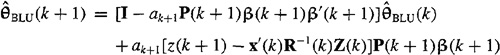
where

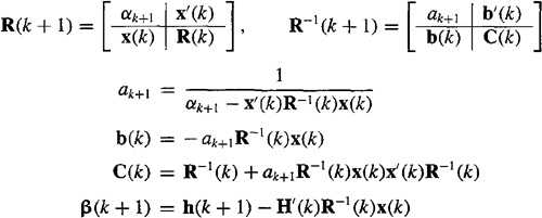
and

P^–1(k + 1) = P^–1(k) + a_k+1β(k + 1)β′(k + 1)

(b) Prepare a flow chart that shows the correct order of computations for this recursive algorithm.

(c) Demonstrate that the algorithm reduces to the usual recursive BLUE when R(k) is diagonal.

(d) What is the recursive WLSE for which W(k + 1) = R^–1(k + 1), when W(k + 1) is nondiagonal but symmetric?