Lesson 4
Least-squares Estimation: Singular-value Decomposition

Summary

The purpose of this lesson is to show how least-squares estimates can be computed using the singular-value decomposition (SVD) of matrix H(k). This computation is valid for both the overdetermined and underdetermined situations and for the situations when H(k) may or may not be of full rank. The SVD of H(k) also provides a practical way to test the rank of H(k).

The SVD of H(k) is also related to the pseudoinverse of H(k). When H(k) is of maximum rank, we show that the pseudoinverse of H(k) reduces to the formula that we derived for in Lesson 3.

When you complete this lesson you will be able to (1) compute using one of the most powerful algorithms from numerical linear algebra, the SVD, and (2) understand the relationship between the pseudoinverse of H(k) and the SVD of H(k).

Introduction

The singular-value decomposition (SVD) of a matrix is a very powerful tool in numerical linear algebra. Among its important uses are the determination of the rank of a matrix and numerical solutions of linear least-squares (or weighted least-squares) problems. It can be applied to square or rectangular matrices, whose elements are either real or complex.

According to Klema and Laub (1980), “The SVD was established for real square matrices in the 1870's by Beltrami and Jordan [see, e.g., MacDuffee (1933, p. 78)], for complex square matrices by Autonne (1902), and for general rectangular matrices by Eckart and Young (1939) (the Autonne-Eckart- Young theorem).” The SVD is presently one of the major computational tools in linear systems theory and signal processing.

As in Lesson 3, our starting point for (weighted) least squares is the generic linear model

(4-1)

Recall that by choosing such that is minimized, we obtained , as

(4-2)

where

(4-3)

Note that in (4-3) was derived using (4-2); hence, it requires H(k) to be of maximum rank. In this lesson we show how to compute even if H(k) is not of maximum rank.

In Lesson 3 we advocated obtaining [or by solving the normal equations . SVD does not obtain by solving the normal equations. When H(k) is of maximum rank, it obtains by computing [H′(k)H(k)]^-1 H′(k), a matrix that is known as the pseudoinverse [of H(k)]. Even when H(k) is not of maximum rank, we can compute using the SVD of H(k).

Some Facts from Linear Algebra

Here we state some facts from linear algebra that will be used at later points in this lesson [e.g., Strang (1988) and Golub and Van Loan (1989)].

[Fl] A unitary matrix U is one for which U′U = I. Consequently, U^-1 = U′.

[F2] Let A be a K x M matrix and r denote its rank; then r ≤ min(K, M).

[F3] Matrix A′A has the same rank as matrix A.

[F4] The eigenvalues of a real and symmetric matrix are nonnegative if that matrix is positive semidefinite. Suppose the matrix is M × M and its rank is r, where r < M; then the first r eigenvalues of this matrix are positive, whereas the last M – r eigenvalues are zero. If the matrix is of maximum rank, then r = M.

[F5] If two matrices V₁ and V₂ are orthogonal, then V₁V₂ = V′₂V₁ = 0.

Singular-Value Decomposition

Theorem 4-1 [Stewart, 1973; Golub and Van Loan, 1989; Haykin, 1991 (Chapter 11)]. Let A be a K × M matrix, and U and V be two unitary matrices. Then

(4-4)

where

(4-5)

and

(4-6)

The σ₁'s are the singular values of A. and r is the rank of A.

Before providing a proof of this very important (SVD) theorem, we note that (1) Theorem 4-1 is true for both the overdetermined (K > M) and underdetermined (K < M) cases, (2) because U and V are unitary, another way of expressing the SVD in (4-4) is

(4-7)

and, (3) the zero matrices that appear in (4-4) or (4-7) allow for matrix A to be less than full rank (i.e., rank deficient); if matrix A is of maximum rank, then U′AV = Σ, or A = UΣV′.

Proof of Theorem 4-1 (overdetermined case). In the overdetermined case K > M, we begin by forming the M × M symmetric positive semidefinite matrix A′A, whose eigenvalues are greater than or equal to zero (see [F4]). Let these eigenvalues be denoted as of, . where (see [F4])

(4-8)

Let v₁, v₂,…, V_M be the set of M × 1 orthonormal eigenvectors of matrix A′A that are associated with eigenvalues , respectively; i.e.,

(4-9)

Collect the M eigenvectors into the M × M matrix V; i.e.,

(4-10)

Matrix V is unitary.

From (4-9), (4-8), and (4-10), we can reexpress the complete system of M equations in (4-9) as

(4-11)

Note that the last M – r columns of A′AV are zero vectors, and, if A′A is of maximum rank so that r = M, then .

Next, form the matrix V′A′AV. In order to understand the structure of this matrix, we interrupt our proof with an example.

EXAMPLE 4-1

Consider the case when A′A is 3 × 3 and r = 2, in which case (4-11) becomes , so that

where we have made use of the orthonormality of the three eigenvectors.

Returning to the proof of Theorem 4-1, we can now express V′A′AV as

(4-12)

where

(4-13)

Σ² is r × r, and zero matrices O₁₂, 0₂₁ and 0₂₂ are r × (M – r), (M – r) × r, and (M – r) × (M – r), respectively.

Because the right-hand side of (4-12) is in partitioned form, we partition matrix V, as

(4-14)

where V₁ is M × r and V₂ is M × (M – r). Because the eigenvectors v_i are orthonormal, we see that

(4-15)

We now equate the left-hand side of (4-12), expressed in partitioned form, to its right-hand side to see that

(4-16a)

and

(4-16b)

Equation (4-16b) can only be true if

(4-17)

Defining the K × r matrix U₁ as

(4-18)

(4-16a) can be reexpressed as

(4-19)

which means that matrix U₁ is unitary.

Next, we create K × M matrix U, where

(4-20)

in which

(4-21a)

and

(4-21b)

From (4-19), (4-21a), (4-21b), and (4-20), we observe that the matrix U (just like matrix V) is unitary.

Now we are ready to examine the matrix U′AV, which appears on the left-hand side of (4-4):

(4-22)

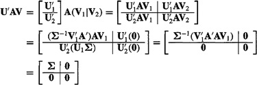
To obtain the first partitioned matrix on the second line of (4-22), we used (4-18) and its transpose and (4-17). To obtain the second partitioned matrix on the second line of (4-22), we used (4-2la). Finally, to obtain the third partitioned matrix on the second line of (4-22), we used (4-16a).

We leave the proof of this theorem in the underdetermined case as Problem 4-7.

Comments

1. The σ₁'s (i = 1, 2,…, r) are called the singular values of matrix A.

2. From (4-11), [F3] and [F4], we see that the rank of matrix A equals the number of its positive singular values; hence, SVD provides a practical way to determine the rank of a matrix.

3. If A is a symmetric matrix, then its singular values equal the absolute values of the eigenvalues of A (Problem 4-4).

4. Vectors v₁, v₂,…, V_M, which were called the set of orthonormal eigenvectors of matrix A′A, are also known as the right singular vectors of A.

5. Let U = (u₁|u₂|…|u_k). Problem 4-7 provides the vectors u₁, u₂,…, u_K with a meaning comparable to that just given to the vectors v₁, v₂,…, v_M.

Using SVD to Calculate

Here we show that can be computed in terms of the SVD of matrix H(k). To begin, we rederive in a waY that is much more general than the Lesson 3 derivation, but one that is only possible now after our derivation of the SVD of a matrix.

Theorem 4-2. Let the SVD of H(k) be given as in (4-4). Even if H(k) is not of maximum rank, then

(4-23)

where

(4-24)

and r equals the rank of H(k).

Proof. We begin with J[k)] from the second line of (3-6) (Stewart, 1973):

Let the SVD of H(k) be expressed as in (4-4). Using the unitary natures of matrices U(k) and V(k), we see that (for notational simplicity, we now suppress the dependency of all quantities on “k”)

(4-26)

Let

(4-27)

and

(4-28)

where the partitioning of m and c conform with the SVD of H given in (4-4). Substituting (4-4), (4-27), and (4-28) into (4-26), we find that

(4-29)

Clearly, for J() to be a minimum, in which case = , c₁ – Σm₁ = 0, from which it follows that

(4-30)

Notice in (4-29) that J() does not depend upon m₂; hence, the actual value of m₂ is arbitrary in relation to our objective of obtaining the smallest value of J(). Consequently, we can choose m₂ = 0. Using m₁ in (4-30) and this zero value of m₂ in (4-27), along with the unitary nature of V, we find that

(4-31)

where we have also used (4-28).

Equation (4-23) can also be written as

(4-32)

where H⁺(k) is the pseudoinverse of H(k):

(4-33)

For discussions about the pseudoinverse and its relationship to , see the Supplementary Material at the end of this lesson.

Theorem 4-3. In the overdetermined case, when N > n

(4-34)

Proof. Using the first term on the right-hand side of (4-31), we see that

(4-35)

But, from (4-18), we see that U′₁ = (HV₁Σ^-1)′; hence,

(4-36)

which can also be expressed as in (4-34).

A computational procedure for obtaining is now clear: (1) compute the SVD of H(k), and (2) compute using (4-34). The generalization of this procedure to is explored in Problem 4-10. Of course, when we know that we are in the overdetermined situation so that we can use (4-34), we only have to determine matrices V and Σ; matrix U does not have to be computed to determine

For numerical methods to accomplish step 1, see Golub and Van Loan (1989) or Haykin (1991). See also the section in this lesson entitled “Computation.”

EXAMPLE 4-2 (Todd B. Leach, Spring 1992)

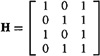
Here we compute using SVD for the overdetermined situation when

(4-37)

We begin by determining the eigenvalues of H'H, where

(4-38)

Observe that

(4-39)

so that the eigenvalues of H'H are at σ² = 6, 2, 0, which means that the rank of H is 2. Next, we determine only those right singular vectors of H'H that comprise V₁ by solving for v_i (i = 1,2) from (4-9). For example σ² = 6 we obtain

(4-40)

Additionally,

(4-41)

We are now able to use (4-34) to compute as

(4-42)

Computation

The following M-files are found directly in MATLAB and will let the end user perform singular-value decomposition, compute the pseudoinverse of a matrix, or obtain the batch WLS estimator.

svd: Computes the matrix singular-value decomposition.

pinv: Moore-Penrose pseudoinverse of a matrix A. Computation is based on svd(A).

Iscov: Least-squares solution in the presence of known covariance. Solves Ax = B using weighted least squares for an overdetermined system of equations, x = lscov(A, B, V), where V = W and W is our WLSE weighting matrix.

Supplementary Material Pseudoinverse

Pseudoinverse

The inverse of a square matrix is familiar to anyone who has taken a first course in linear algebra. Of course, for the inverse to exist, the square matrix must be of maximum rank. SVD can be used to test for this. The pseudoinverse is a generalization of the concept of matrix inverse to rectangular matrices. We use H⁺ to denote the n × N pseudoinverse of N × n matrix H. H⁺ is defined as the matrix that satisfies the following four properties:

(4-43)

Observe that if H is square and invertible, then H⁺ = H^-1. Matrix H⁺ is unique (Greville, 1959) and is also known as the “generalized inverse” of H. According to Greville (1960), the notion of the pseudoinverse of a rectangular or singular matrix (was) introduced by Moore (1920, 1935) and later rediscovered independently by Bjerhammar (1951a, 1951b) and Penrose (1955).

Theorem 4-4. When matrix H is of full rank and N > n (overdetermined case), so that r = min (N, n) = n, then

(4-44a)

When N < n (underdetermined case), so that r = min (N, n) = N, then

(4-44b)

Proof. Note that matrix H must be of full rank for (H′H)^–1 or (HH′)^–1 to exist. To prove this theorem, show that H⁺ in (4-44) satisfies the four defining properties of H⁺ given in (4-43).

We recognize the pseudoinverse of H in (4-44a) as the matrix that premultiplies Z(k) in the formula that we derived for , Eq. (3-11). Note that, when we express as , (4-44b) lets us compute the least-squares estimate in the underdetermined case.

Next we demonstrate how H⁺ can be computed using the SVD of matrix H.

Theorem 4-5. Given an N × n matrix H whose SVD is given in (4-7). Then

(4-45)

where

(4-46)

and r equals the rank of H.

Proof. Here we derive (4-45) for (4-44a); the derivation for (4-44b) is left as a problem. Our goals are to express (H′H)^–1 and H′ in terms of the quantities that appear in the SVD of H. Equation (4-45) will then follow directly from (4-44a).

Observe, from (4-16a) and the unitary nature of V₁, that matrix H′H can be expressed as

(4-47)

Hence,

(4-48)

where we have used [F₁]. Next, solve (4-18) for matrix H, again using the unitary nature of V₁, and then show that

(4-49)

Finally, substitute (4-48) and (4-49) into (4-44a) to see that

(4-50)

Summary Questions

1. The SVD of a full rank matrix A decomposes that matrix into the product:

(a) of three matrices, U′AV

(b) of three matrices UΣV′

(c) LL′

2. In the SVD of matrix A, which of the following are true?

(a) U and V are unitary

(b) A must be of full rank

(c) Σ is a diagonal matrix whose elements may be negative

(d) Σ is a diagonal matrix whose elements must all be positive

(e) The elements of Σ are the eigenvalues of A

(f) The elements of Σ are the singular values of A

3. The rank of matrix A equals:

(a) trace (A)

(b) the number of positive singular values of A′A

(c) the number of positive singular values of A

4. When A is symmetric, then:

(a) its singular values equal the absolute values of its eigenvalues

(b) A^-1 = A

(c) AB = BA

5. can be computed by computing the:

(a) inverse of H(k)

(b) SVD of H(k) and then using (4-34)

(c) the eigenvalues of H(k) and then using (4-34)

6. For the pseudoinverse of H, H⁺, which of the following are true? H⁺:

(a) is the same as H^-1, if H is invertible

(b) satisfies five properties

(c) can be computed using the SVD of H

(d) satisfies four properties

7. can be expressed in terms of H⁺ as:

(a) (HH⁺H)Z(k)

(b) (H⁺H)^-1 H⁺Z(k)

(c) (H⁺HH⁺)Z(k)

Problems

4-1. (David Adams, Spring 1992) Find the SVD of the matrix

4-2. Compute the SVD of the following observation matrix, H(k), and show how it can be used to calculate :

4-3. (Brad Verona, Spring 1992) Given the linear measurement equation Z(k) = H(k)θ + V(k), where Z(k) is a 3 × 1 measurement vector, θ is a 2 × 1 parameter vector, V(k) is a 3 × 1 noise vector, and H(k) is the 3 × 2 observation matrix

Find the least-squares estimator of θ using SVD and the pseudoinverse.

4-4. Prove that if A is a symmetric matrix then its singular values equal the absolute values of the eigenvalues of A.

4-5. (Chanil Chung, Spring 1992) Let A be an m × m Hermitian matrix with orthonormal columns that is partitioned as follows:

Show that if A₁, has a singular vector u with singular value γ, then u is also a singular vector of A₂ with singular value σ, where γ² + σ² = 1.

4-6. (Patrick Lippert, Spring 1992) Singular matrices have long been a source of trouble in the field of robotic manipulators. Consider the planar robot in Figure P4-6, which consists of a revolute joint and two translational joints (commonly known as an RTT arm).

Figure P4-6

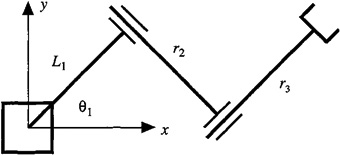
The following matrix P_r describes the position vector of the tip of the arm with respect to the base of the robot:

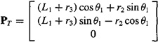
Here we have three degrees of freedom in a system that only has two degrees of freedom (i.e., the arm can only move in the x and y directions). The problem arises when we try to compute the necessary joint velocities to match a desired Cartesian velocity in the following equation:

where J(θ) is the Jacobian matrix of the position vector, dθ(t)/dt = col[[dθ₁(t)/dt, dr₂(t)/dt, dr₃(t)/dt] and v(t) = col [dx(t)/dt, dy(t)/dt, dz(f)/dt].

(a) Find the Jacobian matrix J(θ).

(b) Show that the pseudoinverse of J(θ) is singular.

4-7. Prove SVD Theorem 4-1 for the underdetermined case. Let U = (u₁|u₂|…|u_k); explain why the u_j’s are the left singular vectors of A and are also the eigenvectors of AA′.

4-8. State and prove the SVD theorem for complex data.

4-9. Let A denote a rectangular K × M matrix. For large values of K and M, storage of this matrix can be a serious problem. Explain how SVD can be used to approximate A and how the approximation can be stored more efficiently than storing the entire A matrix. This procedure is known as data compression.

4-10. Demonstrate how SVD can be used to compute the weighted least-squares estimate of θ in the generic linear model (4-1).

4-11. (Charles Pickman, Spring 1992) In many estimation problems that use the linear model Z(k) = H(k)θ + V(k), H(k) is assumed constant and full rank. In practice, the elements of H(k) are measured (or estimated) and include perturbations due to measurement errors. The effects of these perturbations on the estimates need to be determind.

(a) Determine _LS(k) given the following SVD of 4 × 3 matrix H(k)_{4 × 3} and a laboratory measurement of Z(k) = col(1, 1, 1, 1): where U(k)_{4 × 4}, , and V(k)_{3 × 3}, are given, respectively as:

(Hint: Carry the 1 and 1/2 terms throughout all the calculations until the final calculation.)

(b) If the perturbations are on the order of the Σ matrix diagonal values, σ_ii, and directly subtract from all diagonal values, then the H matrix may be rank deficient (a near zero diagonal term exists). What is a reasonable rank to use, given a measurement error on the order of 0.1, 1, 1.5, or 3?

(c) There is a certain amount of error associated with :

Decompose this error into a summation of inner products. Show the derivation and resulting equation.

(d) The error e_LS is a minimum given the available H(k) and Z(k). Calculate its value when the rank of H(k), ρ(H) = 3, using given in part (a). Then assume the H(k) matrix, σ_ii values are perturbed due to measurement errors. Recalculate e_LS when p(H) = 2 and p(H) = 1. Show results for all three cases. Compare the three cases.

4-12. Develop a formula for computing using SVD.

4-13. Prove the truth of the following pseudoinverse facts and related facts:

(a) H′HH⁺ = H′

(b) H⁺HH′ = H′

(c) H′H′⁺H⁺ = H⁺

(d) H⁺H′⁺H′ = H⁺

(e) H⁺⁺ =H

4-14. (Michiel van Nieustadt, Spring 1992) A standard problem in radar theory is the estimation of the number of independent sources in a signal. This is usually done by estimating the rank of a matrix.

Consider p sources and m sensors, where m > p and p is unknown. The jth source sends out a signal with unknown frequency f_j, i.e., S_j(k) = sin(f_jk). The ith sensor receives the sum of the p signals each combined with an unknown scaling factor a_ij. These signal sums are also corrupted by zero-mean Gaussian noise:

where k denotes discrete time, and n_i(k) are unity variance white noises. This equation can also be expressed in matrix form as

r(k) = As(k) + σn(k)

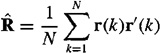
The number of signals can now be estimated as the rank of the matrix R = E{r(k)r′(k)}, which is approximated by the sample covariance

If S denotes the covariance matrix of the signals s, then

Assume that A has full rank p.

(a) Show that R has m – p eigenvalues equal to σ² and p eigenvalues greater than σ². Consequently, the rank of S equals p and can be estimated by looking at the smallest k equal eigenvalues of and estimating p = m – k.

(b) Let p = 2, m = 4, N = 20, f = (1, 2), and

Use SVD to find the eigenvalues of RR′ and then of R when σ = 0.1.

(c) Repeat part (b) when σ = 1.0. Comment on the effect of noise.