Lesson 21
State Estimation: Smoothing (General Results)

Summary

The purpose of this lesson is to develop general formulas for fixed-interval, fixed-point, and fixed-lag smoothers. The structure of our “most useful” fixed-interval smoother is very interesting, in that it is a two-pass signal processor. First, data are processed in the forward direction by a Kalman filter to produce the sequence of innovations Then these innovations are processed in a backward direction by a time-varying recursive digital filter that resembles a backward-running recursive predictor. The noncausal nature of the fixed interval smoother is very apparent from this two-pass structure.

One of the easiest ways to derive both fixed-point and fixed-lag smoothers is by a state-augmentation procedure. In this procedure, a clever choice of additional state variables is made and then a new “augmented” basic state-variable model is created by combining the original basic state-variable model with the state-variable model that is associated with these new states. A Kalman filter is then obtained for the augmented model. By partitioning this Kalman filter’s equations, we obtain the filtered estimates of the augmented states. These filtered estimates turn out to be smoothed estimates of the original states, because of the “clever” choice of these new states.

When you complete this lesson, you will be able to (1) describe a computationally efficient fixed-interval smoother algorithm, and (2) explain how to obtain fixed-point and fixed-lag smoothers by a state augmentation procedure.

Introduction

In Lesson 20 we introduced three general types of smoothers: fixed-interval, fixed-point, and fixed-lag smoothers. We also developed formulas for single- and double-stage smoothers and showed how these specialized smoothers fit into the three general categories. In this lesson we shall develop general formulas for fixed-interval, fixed-point, and fixed-lag smoothers.

Fixed-interval Smoothing

In this section we develop a number of algorithms for the fixed-interval smoothed estimator of x(k), . Not all of them will be useful, because we will not be able to compute with some. Only those with which we can compute will be considered useful.

Recall that

(21-1)

It is straightforward to proceed as we did in Lessons 20, by showing first that

(21-2)

where

(21-3)

and then that

(21-4)

and, finally, that other algorithms for x(kN) are

(21-5)

and

(21-6)

A detailed derivation of these results that uses a mathematical induction proof can be found in Meditch (1969, pp. 216-220). The proof relies, in part, on our previously derived results in Lessons 20, for the single- and double-stage smoothers. The reader, however, ought to be able to obtain (21-4), (21-5), and (21-5) directly from the rules of formation that can be inferred from the Lesson 20 formulas for M(kk + 1) and M(kk + 2) and and .

To compute for specific values of k, all the terms that appear on the right-hand side of an algorithm must be available. We have three possible algorithms for ; however, as we explain next, only one is “useful.”

The first value of k for which the right-hand side of (21-2) is fully available is k = N – 1. By running a Kalman filter over all the measurements, we are able to compute and , so that we can compute . We can now try to iterate (21-2) in the backward direction to see if we can compute , etc. Setting k = N - 2 in (21-2), we obtain

(21-7)

Unfortunately, , which is a single-stage smoothed estimate of , has not been computed; hence, (21-7) is not useful for computing . We, therefore, reject (21-2) as a useful fixed-interval smoother.

A similar argument can be made against (21-5); thus, we also reject (21-5) as a useful fixed-interval smoother.

Equation (21-6) is a useful fixed-interval smoother, because all its terms on its right-hand side are available when we iterate it in the backward direction. For example,

(21-8)

and

(21-9)

Observe how is used in the calculation .

Equation (21-6) was developed by Rauch et al. (1965).

Theorem 21-1. A useful mean-squared fixed-interval smoothed estimator of x(k), , is given by the expression

(21-10)

where matrix A(k) is defined in (20-15), and k = N–1, N – 2,…,0. Additionally, the error-covariance matrix associated with , P(k/N), is given by

(21-11)

where k = N- l.N-2,…,0.

Proof. We have already derived (21-10); hence, we direct our attention to the derivation of the algorithm for P(kN). Our derivation of (21-11) follows the one given in Meditch, 1969, pp. 222-224. To begin, we know that

(21-12)

Substitute (21-10) into (21-12) to see that

(21-13)

Collecting terms conditioned on W on the left-hand side and terms conditioned on k on the right-hand side, (21-13) becomes

(21-14)

Treating (21-14) as an identity, we see that the covariance of its left-hand side must equal the covariance of its right-hand side; hence [in order to obtain (21-15) we use the orthogonality principle to eliminate all the cross-product terms],

(21-15)

or

(21-16)

where . Note that is not a covariance matrix, because . We must now evaluate and Recall that ; thus,

(21-17)

Additionally, , so

(21-18)

Equating (21-17) and (21-18), we find that

(21-19)

Finally, substituting (21-19) into (21-16), we obtain the desired expression for P(kN), (21-11).

A proof of the fact that , k = N, N – 1,…, 0}, is a zero-mean second-order Gauss-Markov sequence is given in the Supplementary Material at the end of this lesson.

EXAMPLE 21-1

To illustrate fixed-interval smoothing and obtain at the same time a comparison of the relative accuracies of smoothing and filtering, we return to Example 19-1. To review briefly, we have the scalar system x(k + 1) = x(k) + w(k) with the scalar measurement z(k + 1) = x(k + 1) + v(k + 1) and p(0) = 50, q – 20, and r = 5. In this example (which is similar to Example 6.1 in Meditch, 1969, p. 225), we choose N = 4 and compute quantities that are associated with , where from (21-10)

(21-20)

k = 3,2, 1, 0. Because Φ = 1 and p(k + lk) = p(kk) + 20,

(21-21)

and, therefore,

(21-22)

Utilizing these last two expressions, we compute A(k) and p(k4) for k = 3,2, 1,0 and present them, along with the results summarized in Table 19-1, in Table 21-1. The three estimation error variances are given in adjacent columns for ease in comparison.

Table 21-1 Kalman Filter And Fixed-Interval Smoother Quantities

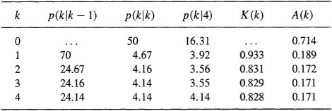
Observe the large improvement (percentage wise) of p(k4) over p(kk). Improvement seems to get larger the farther away we get from the end of our data; thus, p(0|4) is more than three times as small as p(0). Of course, it should be, because p(0) is an initial condition that is data independent, whereas p(0|4) is a result of processing z(l), z(2), z(3), and z(4). In essence, fixed-interval smoothing has let us look into the future and reflect the future back to time zero.

Finally, note that, for large values of k, A(k) reaches a steady-state value, A, where in this example

(21-23)

This steady-state value is achieved for k = 3.

Equation (21-10) requires two multiplications of n x n matrices, as well as a matrix inversion at each iteration; hence, it is somewhat limited for practical computing purposes. The following results, which are due to Bryson and Frazier(1963) and Bierman (1973b), represent the most practical way for computing and also P(kN).

Theorem 21-2. (a)A most useful mean-squared fixed-interval smoothed estimator of x(k), is

(21-24)

where k = N– 1, N – 2,…,1, and n x 1 vector r satisfies the backward-recursive equation

(21-25)

where j = N, N - 1,…, 1 and r(N + 1|N) = 0. Matrix Φ_p is defined in (21-33).

(b) The smoothing error-covariance matrix, P(k|N), is

(21-26)

where k = N–1, N – 2,…,1, and n x n matrix S(j|N), which is the covariance matrix r(j|N), satisfies the backward-recursive equation

(21-27)

where j = N, N - 1,…, 1 and S(N + 1|N) = 0.

Proof (Mendel, 1983, pp. 64-65). (a) Substitute the Kalman filter equation (17-11) for " into Equation (21-10), to show that

(21-28)

Residual state vector r(kN) is defined as

(21-29)

Next, substitute r(k|N and r(k + 1N), using (21-29), into (21-28) to show that

(21-30)

From (17-12) and (17-14) and the symmetry of covariance matrices, we find that

(21-31)

and

(21-32)

Substituting (21-31) and (21-32) into Equation (21-30) and defining

(21-33)

we obtain Equation (21-25). Setting k = N + 1 in (21-29), we establish r(N + l|N) = 0. Finally, solving (21-29) for , we obtain Equation (21-24).

(b) The orthogonality principle in Corollary 13-3 leads us to conclude that

(21-34)

because r(kN) is simply a linear combination of all the observations z(l), z(2),…, z(N). From (21-24) we find that

(21-35)

and, therefore, using (21-34), we find that

(21-36)

where

(21-37)

is the covariance-matrix of r(kN) [note that r(kN) is zero mean]. Equation (21-36) is solved for P(kN) to give the desired result in Equation (21-26).

Because the innovations process is uncorrelated, (21-27) follows from substitution of (21-25) into (21-37). Finally, S(N + lN) = 0 because r(N + lN) = 0.

Equations (21-24) and (21-25) are very efficient; they require no matrix inversions or multiplications of n x n matrices. The calculation of P(kN) does require two multiplications of n x n matrices.

Matrix Φ_p (k + 1, k) in (21-33) is the plant matrix of the recursive predictor (Lesson 16). It is interesting that the recursive predictor and not the recursive filter plays the predominant role in fixed-interval smoothing. This is further borne out by the appearance of predictor quantities on the right-hand side of (21-24). Observe that (21-25) looks quite similar to a recursive predictor [see (17-23)] that is excited by the innovations – one that is running in a backward direction.

Finally, note that (21-24) can also be used for k = N, in which case its right-hand side reduces to , which, of course, is

For an application of the results in Theorem 21-2 to deconvolution, see the Supplementary Material at the end of this lesson.

Fixed-point Smoothing

A fixed-point smoother, , where j = k + 1, k + 2,…, can be obtained in exactly the same manner as we obtained fixed-interval smoother (21-5). It is obtained from this equation by setting N equal to j and then letting j = k + 1, k + 2,…;thus,

(21-38)

where

(21-39)

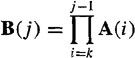
and j = k + 1, k + 2,…. Additionally, we can show that thefixed-point smoothing error-covariance matrix, P(k|j), is computed from

(21-40)

where j = k + l, k + 2,….

Equation (21-38) is impractical from a computational viewpoint, because of the many multiplications of n x n matrices required first to form the A(i) matrices and then to form the B(j) matrices. Additionally, the inverse of matrix P(i + l|i)is needed in order to compute matrix A(i). The following results present a “fast” algorithm for computing . It is fast in the sense that no multiplications of n xn matrices are needed to implement it.

Theorem 21-3. A most useful mean-squared fixed-point smoothed estimator of x(k), where I = 1,2,…, is given by the expression

(21-41)

where

(21-42)

and

(21-43)

Equations (21-41) and (21-43) are initialized byand D_x(k, 1) = P(k/k)Φ’(k +1, k), respectively. Additionally,

(21-44)

which is initialized by P(k|k).

We leave the proof of this useful theorem, which is similar to a result given by Fraser (1967), as an exercise for the reader.

EXAMPLE 21-2

Here we consider the problem of fixed-point smoothing to obtain a refined estimate of the initial condition for the system described in Example 21-1. Recall that p(0|0) = 50 and that by fixed-interval smoothing we had obtained the result p(0|4) = 16.31, which is a significant reduction in the uncertainty associated with the initial condition.

Using Equation (21-40) or (21-44), we compute p(0[l), p(0|2), and p(0|3) to be 16.69, 16.32, and 16.31, respectively. Observe that a major reduction in the smoothing error variance occurs as soon as the first measurement is incorporated and that the improvement in accuracy thereafter is relatively modest. This seems to be a general trait of fixed-point smoothing.

Another way to derive fixed-point smoothing formulas is by the following state augmentation procedure (Anderson and Moore, 1979). We assume that for k ≥ j

(21-45)

which means that x(k) is held constant at the value x(y’) for all k ≥ j. The state equation for state vector x_a(k) is

(21-46)

It is initialized at k = j by (21-45). Augmenting (21-46) to our basic state-variable model in (15-17) and (15-18), we obtain the following augmented basic state-variable model:

(21-47)

and

The following two-step procedure can be used to obtain an algorithm for

1. Write down the Kalman filter equations for the augmented basic state-variable model. Anderson and Moore (1979) give these equations for the recursive predictor; i.e., they find

(21-49)

where k ≥ j. The last equality in (21-49) makes use of (21-46) and (21-45), i.e., Observe that , the fixed-point smoother of x(j), has been found as the second component of the recursive predictor for the augmented model.

2. The Kalman filter (or recursive predictor) equations are partitioned in order to obtain the explicit structure of the algorithm for . We leave the details of this two-step procedure as an exercise for the reader.

Fixed-lag Smoothing

The earliest attempts to obtain a fixed-lag smoother led to an algorithm (e.g., Meditch, 1969) that was later shown to be unstable (Kelly and Anderson, 1971). The following state augmentation procedure leads to a stable fixed-interval smoother for

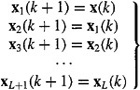
We introduce L + 1 state vectors, as follows: x₁(k + 1) = x(k), x₂(k + 1) = x(k – 1), x₃(k + 1) = x(k – 2),…, x_L+l(k + 1) = x(k – L) [i.e., x_i(k + 1) =x(k + 1 – i), i = 1, 2,…, L + 1]. The state equations for these L + 1 state vectors are

(21-50)

Augmenting (21-50) to our basic state-variable model in (15-17) and (15-18), we obtain yet another augmented basic state-variable model:

(21-51)

Using (21-51), it is easy to obtain the following Kalman filter:

(21-52)

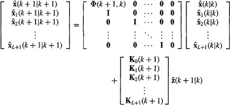
where, for the sake of simplicity, we have assumed that u(k) = 0. Using the facts that x₁(k + 1) = x(k), x₂ (k + 1) = x(k – 1),…, x_L+1 (k + 1) = x(k – L), we see that

(21-53)

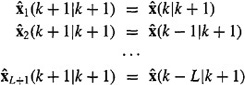
Consequently, (21-52) can be written out as

(21-54)

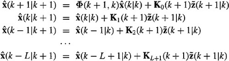
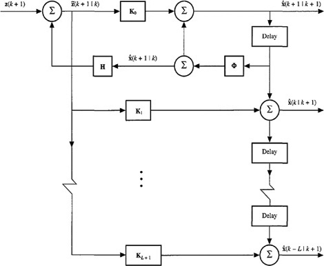
Values for K₀, K₁,…, K_L+1 are obtained by partitioning the Kalman gain matrix equation (17-12). The block diagram given in Figure 21-1 demonstrates that this implementation of the fixed-lag smoother introduces no new feedback loops other than the one that appears in the Kalman filter; hence, the eigenvalues of this smoother are those of the Kalman filter. Because the Kalman filter is stable [this is not only true for the steady-state Kalman filter, but is also true for the non-steady-state Kalman filter; see Kalman (1960) for a proof of this that uses Lyapunov stability theory], this fixedlag smoother is also stable.

Figure 21-1 Fixed-lag smoother block diagram.

Some additional aspects of this fixed-lag smoother are:

1. To compute , we must also compute the L – 1 fixed-lag estimates, , ,…, ; this may be costly to do from a computational point of view.

2. Computation can be reduced by careful coding of the partitioned recursive predictor equations.

Computation

No M-file exists in any toolbox for fixed-interval smoothers; hence, we have prepared the following M-file to do it:

fis: obtains the mean-squared fixed-interval smoothed estimate of the state vector of our basic state-variable model. This model can be time varying or nonstationary.

A complete listing of this M-file can be found in Appendix B.

In this lesson we have also shown how both fixed-point and fixed-lag smoothers can be obtained from a Kalman filter by using state augmentation techniques. The augmented basic state-variable model for fixed-point smoothing is given in (21-47), whereas the basic state-variable model for fixed-lag smoothing is given in (21-51). We can use the M-file kp described in Lesson 17 and listed in Appendix B to compute fixed-point and fixed-lag smoothers using the respective augmented models, or we can use existing M-files in the Control System Toolbox to generate steady-state fixed-point or fixed-lag smoothers, again using the respective augmented models. See Lesson 19 for discussions on the latter.

Supplementary Material

Second-order Gauss-Markov Random Sequences

Suppose we have a stochastic sequence {x(k), k = 0, 1,…} that is defined by the second-order linear vector difference equation

(21-55)

where x(0) and x(1) are jointly Gaussian and {w(k), k = 0, 1,…} is a Gaussian white sequence that is independent of x(0) and x(1).

Because all sources of uncertainty are Gaussian and (21-55) is linear, x(k) must be Gaussian. Additionally, because (21-55) is second order, the conditional probability density function of x at any time point, given the values of x at an arbitrary number of previous time points, depends only on its two previous values; hence, x(k) is a second-order Markov sequence. Note, also, that to go from input w(k) to the state at time k + 2 requires two delays.

Another situation that also leads to a second-order Gauss-Markov sequence is one in which our system is described by the two coupled first-order difference equations:

(21-56)

(21-57)

where, again, all sources of uncertainty are jointly Gaussian. In this case, w(k) is colored noise, a case that is covered more fully in Lessons 22. There are two delays in this system between the input ξ(k) and “output” x(k + 1); hence, the system is second order and is therefore Markov 2.

The state augmentation procedure that is described in Lesson 22 permits us to treat a Markov 2 sequence as an augmented Markov 1 sequence. For additional details, see Meditch (1969).

Next we explain why , is a second-order Markov sequence. We could present a number of detailed analyses to prove that can be expressed in terms of and ; but this is tedious and not very enlightening. Instead, we give a heuristic explanation.

First, we see from (21-24) that depends on both and r(k|N). The recursive predictor, which is given in (17-23), is a first-order Markov sequence, because depends only on . The recursive equation for residual state vector r(k|N), given in (21-25), is a first-order backward-Markovian sequence, because r(j|N) depends only on r(j + 1|N). Finally, as we just noted above, the interrelationship between two first-order coupled Markov sequences is that of a second-order Markov sequence. Note that, in this case, the coupling occurs in the equation for , which plays the role of an output equation for the and r(k|N) systems.

Minimum-variance Deconvolution (MVD)

Here, as in Example 2-6 and 13-1, we begin with the convolutional model

(21-58)

Recall that deconvolution is the signal-processing procedure for removing the effects of h(j) and v(j) from the measurements so that we are left with an estimate of μ(j). Here we shall obtain a very useful algorithm for a mean-squared fixed-interval estimator of μ(j).

To begin, we must convert (21-58) into an equivalent state-variable model.

Theorem 21-4 (Mendel, 1983, pp. 13-14). The single-channel state-variable model

(21-59)

(21-60)

is equivalent to the convolutional sum model in (21-58) when x(0) = 0, μ(0) = 0, h(0) = 0, and

(21-61)

Proof. Iterate (21-59) (see Equation D-49) and substitute the results into (21-60). Compare the resulting equation with (21-58) to see that, under the conditions x(0) = 0, μ(0) = 0, and h(0) = 0, they are the same.

The condition x(0) = 0 merely initializes our state-variable model. The condition μ(0) = 0 means there is no input at time zero. The coefficients in (21-61) represent sampled values of the impulse response. If we are given impulse response data {h(1), h(2),…, h(L)}, then we can determine matrices Φ, γ, and h as well as system order n by applying an approximate realization procedure, such as Kung’s (1978), to {h(1), h(2),…, h(L)}. Additionally, if h(0) ≠ 0, it is simple to modify Theorem 21-4.

In Example 13-1 we obtained a rather unwieldy formula for μ_MS(N). Note that, in terms of our conditioning notation, the elements of μ_MS(N) are μ_MS(k|N), k = 1, 2,…, N. We now obtain a very useful algorithm for μ_MS(kN). For notational convenience, we shorten μ_MS to μ.

Theorem 21-5 (Mendel, 1983, pp. 68-70)

a. A two-pass fixed-interval smoother for μ(k) is

(21-62)

where k = N – 1, N – 2,…, 1.

b. The smoothing error variance, , is

(21-63)

where k = N – 1, N – 2,…, 1. In these formulas r(k|N) and S(k|N) are computed using (21-25) and (21-27), respectively, and E{μ²(k)} = q(k) [here q(k) denotes the variance of μ(k) and should not be confused with the event sequence, which appears in the product model for μ(k)].

Proof

a. To begin, we apply the fundamental theorem of estimation theory, Theorem 13-1, to (21-59). We operate on both sides of that equation with E{·|Z(N)} to show that

(21-64)

By performing appropriate manipulations on this equation, we can derive (21-62) as follows. Substitute and from Equation (21-24) into Equation (21-64), to see that

(21-65)

Applying (17-11) and (16-4) to the state-variable model in (21-59) and (21-60), it is straightforward to show that

(21-66)

Hence, (21-65) reduces to

(21-67)

Next, substitute (21-25) into (21-67), to show that

(21-68)

Making use of Equation (17-12) for K(k), we find that the first and last terms in Equation (21-68) are identical; hence,

(21-69)

Combine Equations (17-13) and (17-14) to see that

(21-70)

Finally, substitute (21-70) into Equation (21-69) to observe that

γ(k|N) = γq(k)γ′r(k + 1|N)

which has the unique solution given by

(21-71)

which is Equation (21-62).

b. To derive Equation (21-63), we use (21-62) and the definition of estimation error ,

(21-72)

to form

(21-73)

Taking the variance of both sides of (21-73) and using the orthogonality condition

(21-74)

we see that

(21-75)

which is equivalent to (21-63).

Observe, from (21-62) and (21-63), that û(kN) and are easily computed once r(k|N) and S(k|N) have been computed.

The extension of Theorem 21-5 to a time-varying state-variable model is straightforward and can be found in Mendel (1983).

EXAMPLE 21-3

In this example we compute , first for a broadband channel IR, h₁(k), and then for a narrower-band channel IR, h₂(k). The transfer functions of these channel models are

(21-76)

and

(21-77)

respectively. Plots of these IRs and their squared amplitude spectra are depicted in Figures 21-2 and 21-3.

Measurements, z(k)(k = 1,2,…, 250, where T – 3 msec), were generated by convolving each of these IRs with a sparse and different spike train (i.e., a Bernoulli-Gaussian sequence) and then adding measurement noise to the results. These measurements, which, of course, represent the starting point for deconvolution, are depicted in Figure 21-4.

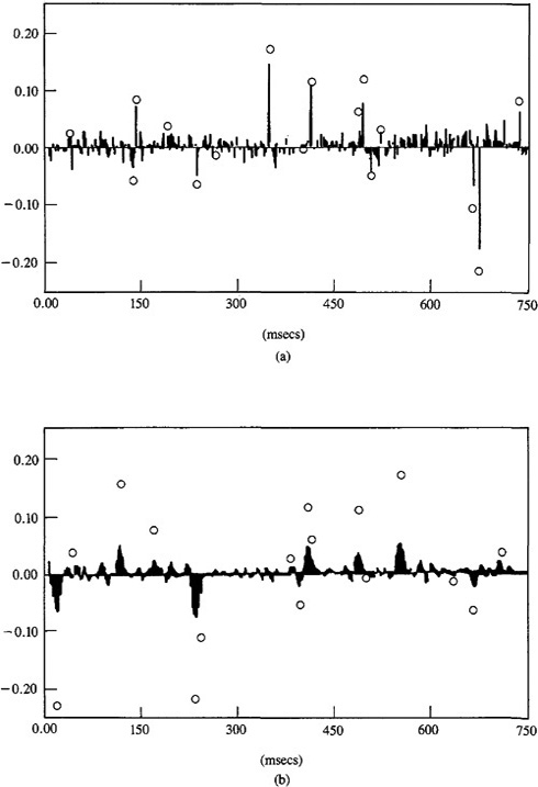
Figure 21-5 depicts . Observe that much better results are obtained for the broadband channel than for the narrower-band channel, even though data quality, as measured by , is much lower in the former case. The MVD results for the narrower-band channel appear “smeared out,” whereas the MVD results for the broadband channel are quite sharp. We provide a theoretical explanation for this effect below.

Observe, also, that tends to undershoot μ,(k). See Chi and Mendel (1984) for a theoretical explanation about why this occurs.

Steady-state MVD Filter

For a time-invariant IR and stationary noises, the Kalman gain matrix, as well as the error-covariance matrices, will reach steady-state values. When this occurs, both the Kalman innovations filter and anticausal μ-filter [(21-62) and (21-25)] become time invariant, and we then refer to the MVD filter as a steady-state MVD filter. In this section we examine an important property of this steady-state filter.

Let h_i(k) and h_μ(k) denote the IRs of the steady-state Kalman innovations and anticausal μ,-filters, respectively. Then

(21-78)

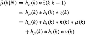
which can also be expressed as

(21-79)

where the signal component of , , is

(21-80)

Figure 21-2 (a) Fourth-order broadband channel IR, and (b) its squared amplitude spectrum (Chi, 1983).

Figure 21-3 (a) Fourth-order narrower-band channel IR, and (b) its squared amplitude spectrum (Chi and Mendel, 1984, © 1984, IEEE).

Figure 21-4 Measurements associated with (a) broadband channel ( = 10) and (b) narrower-band channel ( = 100) (Chi and Mendel, 1984, © 1984, IEEE).

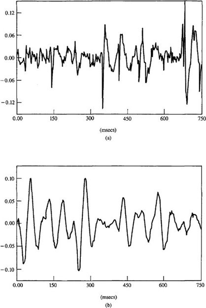
Figure 21-5 for (a) broadband channel ( = 10) and (b) narrower-band channel ( = 100). Circles depict true (k) and bars depict estimate of (k) (Chi and Mendel, 1984, © 1984, IEEE).

and the noise component of , n(kN), is

(21-81)

We shall refer to h_u(k) * h₁(k) as the IR of the MVD filter, h_MV (k); i.e.,

(21-82)

The following result has been proved by Chi and Mendel (1984) for the slightly modified model x(k + 1) = + rµ(k + 1 and x(k) [because of the µ(k +1) input instead of the µ(k) input, h(0) ≠ 0].

Theorem 21-6. In the stationary case:

a. The Fourier transform of h_MV(k) is

(21-83)

where H*(ω) denotes the complex conjugate of H(ωw); and

b. the signal component of , , is given by

(21-84)

where R(k) is the autocorrelation function

(21-85)

in which

(21-86)

Additionally,

(21-87)

We leave the proof of this theorem as an exercise for the reader. Observe that part (b) of the theorem means that is a zero-phase wave-shaped version of µ(k). Observe, also, that R(ω) can be written as

(21-88)

which demonstrates that q/r, and subsequently , is an MVD filter tuning parameter. As so that thus, for high signalto-noise ratios, . → (k) Additionally, when , and once again . Broadband IRs often satisfy this condition. In general, however, is a smeared-out version of µ(k); however, the nature of the smearing is quite dependent on the bandwidth of h(k) and .

EXAMPLE 21-4

This example is a continuation of Example 21-3. Figure 21-6 depicts R(k) for both the broadband and narrower-band IRs, h₁(k) and h₂(k), respectively. As predicted by (21-88), R₁(k) is much spikier than R₂(k) which explains why the MVD results for the broadband IR are quite sharp, whereas the MVD results for the narrower-band IR are smeared out. Note, also, the difference in peak amplitudes for R₁(k) and R₂(k). This explains why underestimates the true values of µ(k) by such large amounts in the narrower-band case (see Figs. 21-5a and b).

Relationship between Steady-State MVD Filter and an Infinite Impulse Response Digital Wiener Deconvolution Filter

We have seen that an MVD filter is a cascade of a causal Kalman innovations filter and an anticausal µ-filter; hence, it is a noncausal filter. Its impulse response extends from k = – ∞ to k = +∞, and the IR of the steady-state MVD filter is given in the time domain by h_MV (k) in (21-82) or in the frequency domain by H_MV (ω) in (21-83).

There is a more direct way for designing an IIR minimum mean-squared error deconvolution filter, i.e., an IIR digital Wiener deconvolution filter, as we describe next.

We return to the situation depicted in Figure 19-4, but now we assume that filter F(z) is an IIR filter, with coefficients {f(j), j = 0, ±1,±2,…};

(21-89)

where µ(k) is a white noise sequence; µ(k), v(k), and n(k) are stationary; and µ,(k) and v(k) are uncorrelated. In this case, (19-44) becomes

(21-90

Using (21-58), the whiteness of µ (k), and the assumptions that µ,(k) and v(k) are uncorrelated and stationary, it is straightforward to show that (Problem 21-13)

(21-91)

Substituting (21-91) into (21-90), we have

(21-92)

We are now ready to solve (21-92) for the deconvolution filter’s coefficients. We cannot do this by solving a linear system of equations because there are a doubly infinite number of them. Instead, we take the discrete-time Fourier transform of (21-92), i.e.,

(21-93)

but, from (21-58), we also know that (Problem 21-13)

Figure 21-6 R(k) for (a) broadband channel ( = 10) and (b) narrower-band channel ( = 100) (Chi and Mendel, 1984, © 1984, IEEE).

(21-94)

Substituting (21-94) into (21-93), we determine F(ω), as

(21-95)

This IIR digital Wiener deconvolution filter (i.e., two-sided least-squares inverse filter) was, to the best of our knowledge, first derived by Berkhout (1977).

Theorem 21-7 (Chi and Mendel, 1984). The steady-state MVD filter, whose IR is given by h_Mv(k), is exactly the same as Berkhout’s IIR digital Wiener deconvolution filter.

The steady-state MVD filter is a recursive implementation of Berkhout’s infinite-length filter. Of course, the MVD filter is also applicable to time-varying and nonstationary systems, whereas his filter is not.

Maximum-likelihood Deconvolution

In Example 14-2 we began with the deconvolution linear model Z(N) = H(N – 1)µ + V(N), used the product model for (i.e.,µ =Q_qr), and showed that a separation principle exists for the determination of and . We showed that first we must determine , after which can be computed using (14-34). Equation (14-34) is terribly unwieldy because of the N x N matrix, that must be inverted. The following theorem provides a more practical way to compute the elements of , where is short for These elements are , k = 1, 2, 3,……N

Theorem 21-8 (Mendel, 1983). Unconditional maximum-likelihood (i.e., MAP) estimates off can be obtained by applying MVD formulas to the state-variable model

(21-96)

(21-97)

where (k) is a MAP estimate q(k).

Proof. Example 14-2 showed that a MAP estimate of q can be obtained prior to finding a MAP estimate of r. By using the product model for µ(k) and , our state-variable model in (21-59) and (21-60) can be expressed as in (21-96) and (21-97). Applying (14-22) to this system, we see that

(21-98)

But, by comparing (21-96) and (21-59) and (21-97) and (21-60), we see that can be found from the MVD algorithm in Theorem 21-5 in which we replace µ(k) by r(k), , and set .

Summary Questions

1. By a “useful” fixed-interval smoother, we mean one that:

(a) runs efficiently

(b) can be computed

(c) is stable

2. By a “most useful” smoother, we mean one that:

(a) can be computed

(b) can be computed with no multiplications of n x n matrices

(c) is stable

3. Smoother error-covariance matrix P(kN):

(a) must be computed prior to processing data

(b) satisfies a forward-running equation

(c) does not have to be calculated at all in order to process data

4. The plant matrix in the backward-running equation for the residual state vector is:

(a) that of the recursive predictor

(b) that of the recursive filter

(c) time invariant

5. In deriving the fixed-lag smoother, we augmented _________versions of x(k) to x(Jfc)?

(a) advanced and delayed

(b) advanced

(c) delayed

6. Deconvolution is the signal-processing procedure for removing the effects of:

(a) h(j) and µ,(j) from the measurements so that we obtain an estimate of v(j)

(b) h(j) and v(j) from the measurements so that we obtain an estimate of µ(j)

(c) µj,(j) and v(j) from the measurements so that we obtain an estimate of h(j)

7. Smoothing error variance shows that MVD:

(a) may not reduce the initial uncertainty q

(b) may sometimes increase initial uncertainty

(c) reduces initial uncertainty

8. The coefficients of a FIR WF are found by solving the normal equations. The coefficients of an IIR WF cannot be found by solving the normal equations, because they:

(a) are a doubly infinite system of equations

(b) are no longer linear

(c) cannot be expressed in matrix form

9. The eigenvalues of the fixed-lag smoother:

(a) are those of the recursive predictor

(b) may lie outside the unit circle

(c) include new stable elements in addition to those of the recursive predictor

10. A second-order Gauss-Markov random sequence is associated with a system that has:

(a) two states

(b) two delays

(c) two moments

11. The IIR digital Wiener deconvolution filter is:

(a) zero phase

(b) causal

(c) all-pass

Problems

21-1. Derive the formula for in (21-5) using mathematical induction. Then derive in (21-6).

21-2. Derive the formula for the fixed-point smoothing error-covariance matrix P(kj) given in (21-40).

21-3. Prove Theorem 21-3, which gives formulas for a most useful mean-squared fixed-point smoother x(k), ,l = 1, 2,….

21-4. Using the two-step procedure described at the end of the section entitled Fixed-point Smoothing, derive the resulting fixed-point smoother equations. Be sure to explain how (jk) and P(jk) are initialized.

21-5. (Kwan Tjia, Spring 1992) Show that, for l = 2, the general result for the mean-squared fixed-point smoothed estimator of x(k), given in Theorem 21-3, reduces to the expression for the double-stage smoother given in Theorem 20-2.

21-6. (Meditch, 1969, Exercise 6-13, p. 245). Consider the scalar system x(k + 1) = 2^-k x(k) + w(k), z(k + 1) = x(k + 1), k = 0, 1,…, where x(0) has mean zero and variance and w(k), k = 0, 1,… is a zero mean Gaussian white sequence that is independent of x(0) and has a variance equal to q.

(a) Assuming that optimal fixed-point smoothing is to be employed to determine x(0j), j = 1,2,…, what is the equation for the appropriate smoothing fiter?

(b) What is the limiting value of p(0j) as j →. ∞

(c) How does this value compare with p(0|0)?

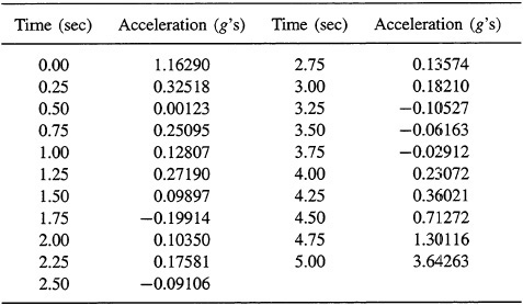
21-7. (William A. Emanuelsen, Spring 1992) (Computation Problem) The state equation for the g accelerations experienced by a fighter pilot in a certain maneuver is

g(k + i) = o.11(k + i)g(k) + w(k)

where w(k) is a noise term to account for turbulence experienced during the maneuver. It is possible to measure g(k) during the maneuver with an accelerometer:

z(k+i) = g(k+l) + v(k+l)

where v(k) is measurement noise in the accelerometer. Given the test data in Table P21-7, and that all noises are zero mean, white, and Gaussian, with variances = 0.04 and = 0.01, determine the fixed-interval smoothed mean-squared estimate of g(k). The mean initial g acceleration is 1.0g and the variance about the mean is unknown.

Table P21-7 Accelerometer Data(z(k)}

21-8. (Mike Walter, Spring 1992) (Computation Problem) Consider the following model:

x₁(k+1) = x₁(k)+x₂(k)

x₂(k + 1) = x₂(k)

z(k + l) = x₁(k + 1) + v(k + 1)

where v(k) is zero-mean white Gaussian noise with = 20, x₁(0) and x₂ (0) are uncorrelated, E{x,(0)} = E{x₂(0)} = 0, and .

(a) Give equations for P(k + 1|k), P(k|k), P(k|N), and

(b) Use a computer to simulate this model for k = 0 to k = 50. Initialize your model with x₁(0) = 1 and x₂ (0) = 1. Produce the following plots: (l)x₁(k) and z(k); (2) P₁₁(k|k) and P₁₁(k|k) for x₁; (3) P₂₂(k|50) and P₂₂(k|50) for x₂; (4) and ; and (5) and

(c) Discuss your results.

21-9. (Richard S. Lee, Jr., Spring 1992) Consider the following linear model that represents a first-order polynomial: Z = H + V, where Z = col (z(0), z(l),…, z(N)), V = col(v(0), v(l),…, v(N)), in which v(k) is zero-mean Gaussian white noise, 0 = col (a, b) and

The values a and b correspond to the parameters in the equation of the line y = a+bx.

(a) Reexpress this model in terms of the basic state-variable model.

(b) Show that the mean-squared fixed-interval smoothed estimator of x(k),, is equal to the mean-squared filtered estimator of x(N),, for all k = 0, 1,…, N. Explain why this is so.

21-10.(Lance Kaplan, Spring 1992) Consider the system

x(k + 1) = Φ(k + 1, k)x(k)

z(k + 1) = H(k + 1)x(k + 1) + v(k + 1)

where (k + 1, k) is full rank for all k.

(a) Show that, when calculating for l = 1, 2,…, then Equation (21-41) yields N_x(k|k + l) = ^-1(k + l, k)K(k + l), where (k + l, k) = (k + l, k + l -1)(k + l - 1, k + l - 2)… (k + 1, k).

(b) Let y(k) = ^-1 (k, 0)x(k) for l = 1, 2, Rewrite the state equations in terms of the new state vector y(k).

(c) Show that N_y(kk + 1) =K(k + 1).

(d) How do the smoothed estimates (kk + e) relate to the filtered estimates (k + lk + e

(e) How do the smoothed estimates relate to the filtered estimates x(k + lk + e)?

21-11. Prove Theorem 21-6. Explain why part (b) of the theorem means that is a zero-phase wave-shaped version of (k).

21-12. This problem is a memory refresher. You probably have either seen or carried out the calculations asked for in a course on random processes.

(a) Derive Equation (21-92).

(b) Derive Equation (21-95).

21-13. (James E. Leight, Fall 1991) Show the details of the proof of Theorem 21-4.

21-14. (Constance M. Chintall, Fall 1991) Determine H_MV(ω) and R(ω) when H(ω) = l/(α + jω). Do this for α = 10 and SNR = 1 and α = 100 and SNR = 0.01. Discuss your results.

21-15. (Gregg Isara and Loan Bui, Fall 1991) Write the equations for (kN) for the following single-channel state-variable model:

x(k + 1) = 0.667x(k) + 3r(k)

z(k + 1) = 0.25x(k + 1) + v(k + 1)

where the variance of r(k) is 4, m_v (k) = 0, and Draw a flow chart for the implementation of