Lesson 24
Iterated Least Squares and Extended Kalman Filtering

Summary

This lesson is devoted primarily to the extended Kalman filter (EKF), which is a form of the Kalman filter “extended” to nonlinear dynamical systems of the form described in Lessons 23. We show that the EKF is related to the method of iterated least squares (ILS), the major difference being that the EKF is for dynamical systems, whereas ILS is not.

We explain ILS for the model z(k) = f(θ, k) + v(k), k = 1, 2,…, N, where the objective is to estimate θ from the measurements. A four-step procedure is given for ILS, from which we observe that in each complete cycle of this procedure we use both the nonlinear and linearized models and that ILS uses the estimate obtained from the linearized model to generate the nominal value of θ about which the nonlinear model is relinearized.

The notions of relinearizing about a filter output and using both the nonlinear and linearized models are also at the very heart of the EKF. The EKF is developed in predictor-corrector format. Its prediction equation is obtained by integrating the nominal differential equation associated with x*(t), from t_k to t_k+1. To do this, we learn that , whereas . The corrector equation is obtained from the Kalman filter associated with the discretized perturbation state-variable model derived in Lessons 23. The gain and covariance matrices that appear in the corrector equation depend on the nominal x*(t) that results from prediction, .

An iterated EKF is an EKF in which the correction equation is iterated a fixed number of times. This improves the convergence properties of the EKF, because convergence is related to how close the nominal value of the state vector is to its actual value.

When you have completed this lesson, you will be able to (1) explain the method of iterated least squares (ILS); (2) derive and use the extended Kalman filter (EKF); (3) explain how the EKF is related to ILS; and (4) apply the EKF to estimate parameters in a state-variable model.

Introduction

This lesson is primarily devoted to the extended Kalman filter (EKF), which is a form of the Kalman filter “extended” to nonlinear dynamical systems of the type described in Lessons 23. We shall show that the EKF is related to the method of iterated least squares (ILS), the major difference being that the EKF is for dynamical systems, whereas ILS is not.

Iterated Least Squares

We shall illustrate the method of ILS for the nonlinear model described in Example 2-5, i.e., for the model

(24-1)

where k = 1,2,…, N.

Iterated least squares is basically a four-step procedure.

1. Linearize f (θ, k) about a nominal value of θ, θ*. Doing this, we obtain the perturbation measurement equation

(24-2)

where

(24-3)

(24-4)

and

(24-5)

2. Concatenate (24-2) and compute using our Lesson 3 formulas.

3. Solve the equation

(24-6)

for , i.e.,

(24-7)

4. Replace θ* with and return to step 1. Iterate through these steps until convergence occurs. denote estimates of θ obtained at the ith and (i + 1)st iterations, respectively. Convergence of the ILS method occurs when

(24-8)

where ∈ is a prespecified small positive number.

We observe, from this four-step procedure, that ILS uses the estimate obtained from the linearized model to generate the nominal value of θ about which the nonlinear model is relinearized. Additionally, in each complete cycle of this procedure, we use both the nonlinear and linearized models. The nonlinear model is used to compute z*(k) and subsequently δz(k), using (24-3).

The notions of relinearizing about a filter output and using both the nonlinear and linearized models are also at the very heart of the EKE.

Extended Kalman Filter

The nonlinear dynamical system of interest to us is the one described in Lessons 23. For convenience to the reader, we summarize aspects of that system next. The nonlinear state-variable model is

(24-9)

(24-10)

Given a nominal input u*(t) and assuming that a nominal trajectory x*(t) exists, x*(t) and its associated nominal measurement satisfy the following nominal system model:

(24-11)

(24-12)

Letting δx(t) = x(t) – x*(t), δu(t) = u(t) – u*(t), and δz(t) = z(t) – z*(t), we also have the following discretized perturbation state-variable model that is associated with a linearized version of the original nonlinear state-variable model:

(24-13)

(24-14)

In deriving (24-13) and (24-14), we made the important assumption that higher-order terms in the Taylor series expansions of f[x(t), u(t), t] and h[x(t), u(t), t] could be neglected. Of course, this is only correct as long as x(t) is “close” to x*(t) and u(t) is “close” to u*(t).

As discussed in Lessons 23, if u(t) is an input derived from a feedback control law, so that u(t) = u[x(t), t], then u(t) can differ from u*(t), because x(t) will differ from x*(t). On the other hand, if u(t) does not depend on x(t), then usually u(t) is the same as u*(t), in which case δu(t) = 0. We see, therefore, that x*(t) is the critical quantity in the calculation of our discretized perturbation state-variable model.

Suppose x*(t) is given a priori; then we can compute predicted, filtered, or smoothed estimates of δx(k) by applying all our previously derived estimators to the discretized perturbation state-variable model in (24-13) and (24-14). We can precompute x*(t) by solving the nominal differential equation (24-11). The Kalman filter associated with using a precomputed x*(t) is known as a relinearized KF.

A relinearized KF usually gives poor results, because it relies on an open-loop strategy for choosing x*(t). When x*(t) is precomputed, there is no way of forcing x*(t) to remain close to x(t), and this must be done or else the perturbation state-variable model is invalid. Divergence of the relinearized KF often occurs; hence, we do not recommend the relinearized KF.

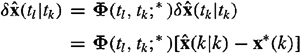
The relinearized KF is based only on the discretized perturbation state-variable model. It does not use the nonlinear nature of the original system in an active manner. The extended Kalman filter relinearizes the nonlinear system about each new estimate as it becomes available; i.e., at k = 0, the system is linearized about . Once z(1) is processed by the EKF, so that is obtained, the system is linearized about . By “linearize about ,” we mean is used to calculate all the quantities needed to make the transition from to and subsequently . This phrase will become clear later. The purpose of relinearizing about the filter’s output is to use a better reference trajectory for x*(t). Doing this, will be held as small as possible, so that our linearization assumptions are less likely to be violated than in the case of the relinearized KF.

The EKF is developed in predictor-corrector format (Jazwinski, 1970). Its prediction equation is obtained by integrating the nominal differential equation for x*(t). from t_k to t_k+1. To do this, we need to know how to choose x*(t) for the entire interval of time t ∈ [t_k, t_k+1]. Thus far, we have only mentioned how x*(t) is chosen at t_k, i.e., as .

Theorem 24-1. As a consequence of relinearizing about (k = 0, 1,…),

(24-15)

This means that

(24-16)

Before proving this important result, we observe that it provides us with a choice of x*(t) over the entire interval of time t ∈ [t_k, t_k+1], and it states that at the left-hand side of this time interval , whereas at the right-hand side of this time interval . The transition from to will be made using the EKF’s correction equation.

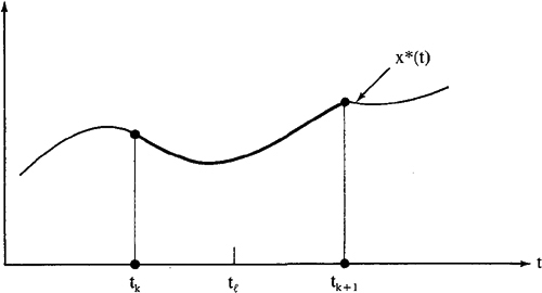
Proof. Let t₁ be an arbitrary value of t lying in the interval between t_k and t_k+1 (see Figure 24-1). For the purposes of this derivation, we can assume that δu(k) = 0 [i.e., perturbation input δu(k) takes on no new values in the interval from t_k to t_k+1; recall the piecewise-constant assumption made about u(t) in the derivation of (23-38)]; i.e.,

Figure 24-1 Nominal state trajectory x*(t).

(24-17)

Using our general state-predictor results given in (16-14), we see that (remember that k is short for t_k, and that t_k+1 – t_k does not have to be a constant; this is true in all of our predictor, filter, and smoother formulas)

(24-18)

In the EKF we set ; thus, when this is done,

(24-19)

and, because t_l ∈ [t_k, t_k+1],

(24-20)

which is (24-15). Equation (24-16) follows from (24-20) and the fact that .

We are now able to derive the EKF. As mentioned previously, the EKF must be obtained in predictor-corrector format. We begin the derivation by obtaining the predictor equation for .

Recall that x*(t) is the solution of the nominal state equation (24-11). Using (24-16) in (24-11), we find that

(24-21)

Integrating this equation from t = t_k to t = t_k+1, we obtain

(24-22)

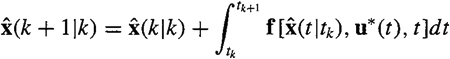
which is the EKF prediction equation. Observe that the nonlinear nature of the system’s state equation is used to determine The integral in (24-22) is evaluated by means of numerical integration formulas that are initialized by .

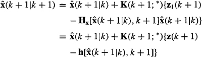
The corrector equation for is obtained from the Kalman filter associated with the discretized perturbation state-variable model in (24-13) and (24-14) and is

(24-23)

As a consequence of relinearizing about , we know that

(24-24)

(24-25)

and

(24-26)

Substituting these three equations into (24-23), we obtain

(24-27)

which is the EKF correction equation. Observe that the nonlinear nature of the system’s measurement equation is used to determine . One usually sees this equation for the case when δu = 0, in which case the last term on the right-hand side of (24-27) is not present.

To compute , we must compute the EKF gain matrix K(k + 1;*). This matrix, as well as its associated P(k + 1|k;*) and P(k + 1|k + 1;*) matrices, depend on the nominal x*(t) that results from prediction, Observe, from (24-16), that x*(k + 1) = and that the argument of K in the correction equation is k + 1; hence, we are indeed justified to use as the nominal value of x* during the calculations of K(k + 1;*), P(k + 1|k;*), and P(k + 1|k + 1;*). These three quantities are computed from

(24-28)

(24-29)

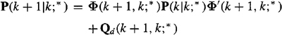
(24-30)

Remember that in these three equations * denotes the use of .

The EKF is very widely used, especially in the aerospace industry; however, it does not provide an optimal estimate of x(k). The optimal estimate of x(k) is still E{x(k)|Z(k)}, regardless of the linear or nonlinear nature of the system’s model. The EKF is a first-order approximation of E{x(k)|Z(k)} that sometimes works quite well, but cannot be guaranteed always to work well. No convergence results are known for the EKF; hence, the EKF must be viewed as an ad hoc filter. Alternatives to the EKF, which are based on nonlinear filtering, are quite complicated and are rarely used.

A flow chart for implementation of the EKF is depicted in Figure 24-2.

Figure 24-2 EKF flow chart.

The EKF is designed to work well as long as δx(k) is “small”. The iterated EKF (Jazwinski, 1970), depicted in Figure 24-3, is designed to keep δx(k) as small as possible. The iterated EKF differs from the EKF in that it iterates the correction equation L times until . Corrector 1 computes K(k + 1;*), P(k + 1|k;*), and P(k + 1|k + 1;*) using x* = ; corrector 2 computes these quantities using ; correctors computes these quantities using ; etc.

Figure 24-3 Iterated EKF. All the calculations provide us with a refined estimate of x(k + 1), starting with

Often, just adding one additional corrector (i.e., L = 2) leads to substantially better results for than are obtained using the EKF.

Application to Parameter Estimation

One of the earliest applications of the extended Kalman filter was to parameter estimation (Kopp and Orford, 1963). Consider the continuous-time linear system

(24-31a)

(24-31b)

Matrices A and H contain some unknown parameters, and our objective is to estimate these parameters from the measurements z(t_i) as they become available.

To begin, we assume differential equation models for the unknown parameters, i.e., either

(24-32a)

(24-32b)

or

(24-33a)

(24-33b)

In the latter models n_i(t) and n_j(t) are white noise processes, and we often choose c_t = 0 and d_j = 0. The noises n_i(t) and n_j(t) introduce uncertainty about the “constancy” of the a_t and h_j parameters.

Next, we augment the parameter differential equations to (24-31a) and (24-31b). The resulting system is nonlinear, because it contains products of states [e.g., a_i(t)x_i(t)]. The augmented system can be expressed as in (24-9) and (24-10), which means we have reduced the problem of parameter estimation in a linear system to state estimation in a nonlinear system.

Finally, we apply the EKF to the augmented state-variable model to obtain .

Ljung (1979) has studied the convergence properties of the EKF applied to parameter estimation and has shown that parameter estimates do not converge to their true values. He shows that another term must be added to the EKF corrector equation in order to guarantee convergence. For details, see his paper.

EXAMPLE 24-1

Consider the satellite and planet Example 23-1, in which the satellite’s motion is governed by the two equations

(24-34)

and

(24-35)

We shall assume that m and y are unknown constants and shall model them as

(24-36)

(24-37)

Defining we have

(24-38)

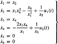
Now,

(24-39)

We note, finally, that the modeling and augmentation approach to parameter estimation, just described, is not restricted to continuous-time linear systems. Additional situations are described in the exercises.

Computation

There is no M-file available to do extended Kalman filtering. Using the flow chart that is given in Figure 24-2, it is straightforward to create such an M-file. It is best, in practice, to use an iterated EKF, with at least one iteration. Remember, though, that both the EKF and IEKF use a linearized and discretized system, which is time varying. See Lesson 17 for a Kalman filter for such a system.

Supplementary Material
EKF for a Nonlinear Discrete-time System

Sometimes we begin with a description of a system directly in the discrete-time domain. An EKF can also be developed for such a system. Consider the nonlinear discrete-time system

(24-40)

(24-41)

where wk and v(k) are Gaussian random sequences. Because this is already a discrete-time system, we only have to linearize it prior to obtaining the EKF formulas. We linearize the state equation about because we will go from the filtered estimate, to the predicted estimate . We linearize the measurement equation about because we will go from the just-computed predicted value of x(k + 1) to its filtered value, .

The linearized state and measurement equations are

(24-42)

(24-43)

The predictor equation is obtained by applying E{-|Z(k)}, to the linearized state equation, i.e.,

(24-44)

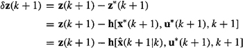
The correction equation is obtained by first reexpressing the linearized measurement equation as

(24-45)

were

(24-46)

and then applying the regular KF correction equation to the linearized system, i.e.,

(24-47)

Equations (24-44) and (24-47) constitute the EKF equations for the original nonlinear discrete-time system. Note that F_x[, k] plays the role of Φ and H_x[, k + 1] plays the role of H in the matrix equations for K(k + 1;*), P(k + l|k;*), and P(k + 1|k + 1;*). Matrices Q and R do not change for this system because it is already a discrete-time system.

Summary Questions

1. The Kalman filter associated with precomputed x*(r) is known as a:

(a) nominal KF

(b) extended KF

(c) relinearized KF

2. The extended KF relinearizes the nonlinear system:

(a) about each new estimate as it becomes available

(b) only about filtered estimates

(c) only about predicted estimates

3. The prediction equation of the EKF is obtained by:

(a) applying the KF prediction equation to the perturbation state-variable model

(b) integrating the nominal differential equation for x*(t), from t_k to t_k+l

(c) setting for all t ∈ [t_k, t_k+1]

4. The corrector equation of the EKF is obtained by:

(a) integrating the measurement equation from t_k to t_k+1

(b) setting for all t ∈ [t_k, t_k+1]

(c) applying the KF corrector equation to the perturbation state-variable model

5. When some parameters that appear in the plant matrix of a linear system are unknown, and they are modeled by linear state equations:

(a) the EKF converges to true values of the unknown parameters

(b) the resulting augmented system is nonlinear

(c) a KF can be used to estimate the parameters

6. In ILS, the nonlinear model is used to compute:

(a) θ*

(b) z*(k)

(c) θ* and z*(k)

7. In the iterated EKF, the:

(a) corrector equation of the EKF is iterated

(b) prediction equation of the EKF is iterated

(c) prediction and correction equations of the EKF are iterated

Problems

24-1. In the first-order system, x(k + 1) = ax(k) + w(k), and z(k + 1) = x(k + 1) + v(k + l), k =1, 2,…, N, a is an unknown parameter that is to be estimated. Sequences w(k) and v(k) are, as usual, mutually uncorrelated and white, and w(k) ∼ N(w(k); 0, 1) and v(k) ∼ N(v(k); 0, ). Explain, using equations and a flow chart, how parameter a can be estimated using an EKF. (Hint: Use the EKF given in the Supplementary Material at the end of this lesson.)

24-2. Repeat the preceding problem where all conditions are the same except that now w(k) and v(k) are correlated, and .

24-3. The system of differential equations describing the motion of an aerospace vehicle about its pitch axis can be written as (Kopp and Orford, 1963)

where , which is the actual pitch rate. Sampled measurements are made of the pitch rate, i.e.,

Noise v(t_i) is white and Gaussian, and is given. The control signal u(t) is the sum of a desired control signal u*(t) and additive noise, i.e.,

The additive noise δu(t) is a normally distributed random variable modulated by a function of the desired control signal, i.e.,

where w₀(t) is zero-mean white noise with intensity . Parameters a₁(t), a₂(t) and a₃(t) may be unknown and are modeled as

In this model the parameters α_i(t) are assumed given, as are the a priori values of a_i(t) , and w_i(t) are zero-mean white noises with intensities .

(a) What are the EKF formulas for estimation of x₁, x₂, a₁, and a₂, assuming that a₃ is known?

(b) Repeat part (a) but now assume that a₃ is unknown.

24-4. Refer to Problem 23-7. Obtain the EKF for:

(a) Equation for the unsteady operation of a synchronous motor, in which C and p are unknown,

(b) Buffing’s equation, in which C, α, and β are unknown,

(c) Van der Pol’s equation, in which ∈, is unknown,

(d) Hill’s equation, in which a and b are unknown.

24-5. (Richard W. Baylor, Spring 1992) Obtain the EKF for a series RLC network in which noisy measurements are made of current, i(t), and we wish to estimate R, L, and C as well as the network’s usual states. The equation for this system is

where v(t) is voltage. Be sure to include the discretization of this continuous-time system.

24-6. (Patrick Lippert, Spring 1992) Given the RTT robotic arm with r₃ = L₂ (see also Problem 4-6, by Lippert), where L₂ is a constant length, we can use the theory of differential kinematics to relate the angular velocities of the robot arm to the Cartesian velocities of the tip of the robot arm. The equations of motion are

Assume that we have sampled measurements of the actuator signals θ_i(t) and r₂(t). Define the state-variable model and the necessary quantities needed for computation by an EKF.