Harmonic distortion and inter-modulation

In the recognition of sounds, our ears use both the fundamental and its harmonics. Harmonics, as already explained, are integer multiples of the fundamental, and thus the two are closely related. By emphasizing harmonics, we increase the definition of sounds. Lower harmonics are louder than higher harmonics. For example, the second harmonic is louder than the 20th harmonic. Due to their relatively loud level, the few low-order harmonics have some extra importance. The second harmonic is an octave above the fundamental, and the fourth harmonic is two octaves above the fundamental. Being octave-related to the fundamental, both harmonics are considered musical—emphasizing them tends to give appealing results. The third and fifth harmonics are also important, but neither is octave-related to the fundamental—both tend to produce a slightly more colorful sound.

A linear device is one that has perfect proportionality between input and output. The transfer curve of such a device is one straight line. An example of a nonlinear device is a compressor with any ratio other than 1:1. When a signal passes through a nonlinear system, different kinds of distortion are produced. The less linear the system, the more profound the distortion. One type of distortion is harmonic distortion—essentially, added harmonics. Analog components are incapable of being perfectly linear. A specification called total harmonic distortion (THD) measures the harmonic distortion content produced by an analog device under standard test conditions. There are different flavors to analog distortion. The ratio between the low-order harmonics produced by a tube is different from that produced by a transistor. This is a major contributor to the different sounds that a tube and solid-state equipment produce. Although technically speaking the lower the distortion the better, harmonic distortion is an intimate part of the analog sound in general and the charac teristics of analog gear in particular. Digital systems are capable of being perfectly linear and thus might not produce harmonic distortion. Although it is technically superior, many find the digital sound lifeless and pale.

Another type of distortion is inter-modulation. Like total harmonic distortion, it can be measured and the specification given is simply called inter-modulation (IMD). Just like harmonic distortion, inter-modulation distortion involves additional frequencies, but unlike harmonic distortion these are not necessarily harmonically related to the sound. Therefore, inter-modulation is often considered harsh and it is mostly unwanted. Yet, it is an inseparable part of any nonlinear system.

The problem with distortion in the digital domain

Often distortion produced within an analog system is more musical than that produced within a digital system. The reason for this originates from the fact that analog systems do not have a frequency limit like digital systems do. The highest frequency a digital system can accommodate is called the Nyquist frequency, and it is always half the sample rate. The problem with digital systems is that any content produced within the system that exceeds the Nyquist frequency mirrors around it. For example, say we have a system running at a sample rate of 44,100 Hz. The highest frequency such a system can accommodate is 22,050 Hz (the Nyquist frequency). Then, say an 8 kHz sine wave is distorted. The resultant harmonic distortion would include a second harmonic at 16 kHz and a fourth harmonic at 32 kHz—both have an octave relationship with the fundamental. However, since the 32 kHz harmonic is higher than the Nyquist frequency, it will mirror around it, resulting in an alias frequency at 12.1 kHz. This frequency is not harmonically related to the 8 kHz fundamental and will produce a harsh sound. On the same basis, any distortion content that exceeds the Nyquist frequency creates aliasing frequencies below it. On an analog system, no such thing happens—any distortion content above 20 kHz is simply unheard.

We can minimize the harsh aliasing phenomenon of digital processing by using higher sample rates. If, for example, the sample rate of the system above was 88.2 kHz, the Nyquist frequency would be 44.1 kHz. This means that the 32 kHz harmonic would not alias—it simply would not be heard. Even content that does alias might do so into the inaudible range between 20 and 44.1 kHz. With 88.2 kHz, only content above 68.2 kHz would alias back into the audible frequency range. The problem with using higher sample rates is that more samples have to be processed. Compared to a sample rate of 44.1 kHz, an 88.2 kHz audio will require twice the samples processed, which essentially halves the processing capabilities of the CPU (or any other digital processor, for that matter). In practice, the actual processing overhead in using higher sample rates can be more than initially expected—some plugins will need to perform substantially more calculations in order to operate at higher sampling rates.

High-quality plugin developers take this aliasing problem into account in their designs by implementing internal upsampling and then downsampling. Essentially, even if the project’s sample rate is 44.1 kHz, the plugin upsamples the audio to, say, 176.4 kHz (4×). This results in a new Nyquist frequency of 88.2 kHz, and only content above 150.4 kHz will alias back into the audible frequency range. The plugin then performs its processing, which might produce content above the original Nyquist frequency—22.05 kHz. Then any content above 20 kHz is removed using an anti-aliasing filter (essentially a high-quality LPF) and the audio is downsampled back to the original project’s sample rate. This way, any content that would otherwise alias back into the audible range is simply removed.

Parallel distortion

Just like the parallel compression technique, where a compressed version is layered underneath the original, signals are sometimes distorted and then layered below the original. This gives us added control over the amount of distortion being added. Consequently, this lets us drive the distortion harder to produce a stronger effect, but then layer it underneath at lower levels so it is not too obvious or crude.

Gain controls

As already described in Chapter 10, a boost on the gain control, affecting the signal early in the signal path, can overload successive components. In the analog domain, we usually speak first of overloading, which mostly adds subtle distortion, and only then saturation, which can produce drastic distortion. The nature of solid-state components is that they provide increasing distortion with gain. Tube equipment tends to produce a very appealing distortion up to a specific point, where the system seems to “break” and produce very undesired clicks. Tapes can be overloaded using the same principle by boosting the input signal. Bipolar transistors, FET, tube, and tape distortion all have different qualities as they all produce different harmonic content. Also, the more each system overloads, the more compression occurs, which makes the overall effect even more appealing.

Digital clipping

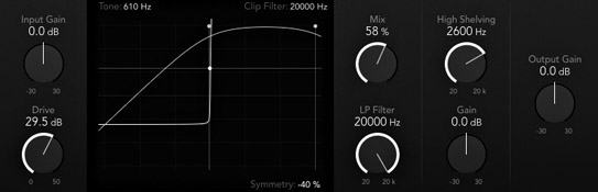
Figure 25.1 The Logic Clip Distortion plugin.

Of all the types of distortion, digital clipping is probably the least appealing. The harsh limiting of audio exceeding the 0 dB threshold on a digital system can produce extremely unpleasant sound, especially if the added content aliases. There are also different types of digital clipping, where differences are dependent on what happens to signals that exceed the system limit. On most floating-point systems, these signals are trimmed to the highest possible value (simply hard-limiting). However, different integer notations can produce different results, where exceeding signals can alias around the highest sample value; they can be displaced to the bottom of the value range or displaced across the zero line.

Generally speaking, clipping tends to produce the strongest type of distortion. Some plugins try to imitate the clipping sound of analog devices by introducing additional processing along with the basic digital clipping. The clip distortion in Figure 25.1 is one of them. It is worth noting the “Mix” control, which lets us blend the undistorted and distorted sounds.

Short attack and release on dynamic range processors

In Chapter 17, which covered compressors, we saw that a short attack and release can act within the cycle of low frequencies, thus altering the shape of the waveform and producing distortion (refer to Figure 17.29 for a demonstration of this). This type of distortion is not reserved solely for compressors and can be produced by short time constants on any dynamic range processor. We can use this type of distortion to add some warmth and definition to instruments with low-frequency content, notably basses.

Wave shapers

A wave shaper is a pure implementation of a transfer curve. Essentially, the signal passes through a transfer characteristics function over which we have some control. This is somewhat similar to a dynamic range processor with no time constants and an unrestricted transfer curve. Wave shapers are not very common and might be a sub-facility within a different effect. However, they can produce extremely interesting results that can be used in subtle amounts for gentle enhancements or in a drastic form for creative effect.

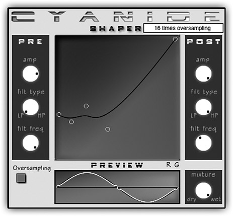
Figure 25.2 The Smartelectronix Cyanide 2 plugin (donationware).

Bit reduction

Early digital samplers that emerged around the early 1980s had low specs compared with those used today—in addition to low sample rates, they were designed around 8-bit (and later 12-bit) samples. Even now, the 8-bit sound is much sought after in genres such as hip-hop, where many find the lo-fi sound of drum samples appealing.

When we discussed software mixers in Chapter 11, we discussed the importance of dither, which rectifies the distortion caused by bit reduction. Unsurprisingly, like many other areas in mixing where we are after the “technically wrong” and the less precise sound, bit reduction can also have an appealing effect. Essentially, a bit reduction process simply reduces the bit depth of digital audio. Although within the audio sequencer the audio is still represented by 32-bit float numbers, sample values are quantized to the steps of the target bit depth. For example, reduction to 1 bit would produce 32-bit float values of 1.0 and –1.0 only (in practice, however, most processors also output 0.0 as a possible sample value). This process produces quantization distortion, where the lower the target bit depth is, the more the distortion. Clearly, we wish to keep this distortion, so no dither is applied. Just like with drum samples, bit reduction can be used to give a lo-fi sense to various instruments. It can also be used as a creative effect.

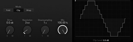
Figure 25.3 The Logic BitCrusher. This plugin combines bit reduction, three-mode clipping distortion, and digital downsampling. In this screenshot, only the reduction to three bits is utilized. The eight quantization steps that would affect a sine waveform are visible on the display.

Amp simulators

A famous mixing practice in the analog domain is called re-amping—feeding a guitar recording during mixdown back into a guitar amp so a different sound texture and distortion can be created. Mostly, the signal sent to the amps during mixdown is the direct recording (before any pedals or amp). Many plugins nowadays are designed to imitate the sound of classic guitar cabinets, and usually these plugins also include other guitar processors such as tremolos, compressors, gates, echo engines, and guitar reverbs. When there is a direct recording of a guitar, we can easily choose the final guitar sound during mixdown (together with the cabinet recording, perhaps replacing it).

Even before the digital age, re-amping was not limited to guitars. Sometimes engineers sent vocals, drums, or other tracks into a guitar amplifier (or guitar pedals), using the amp as a distortion or effects unit. Using the same principle, an amp simulator plugin can be used to distort any type of material. Like any other type of distortion, subtle settings can be useful for gentle enhancements and more trashy settings for more drastic results.

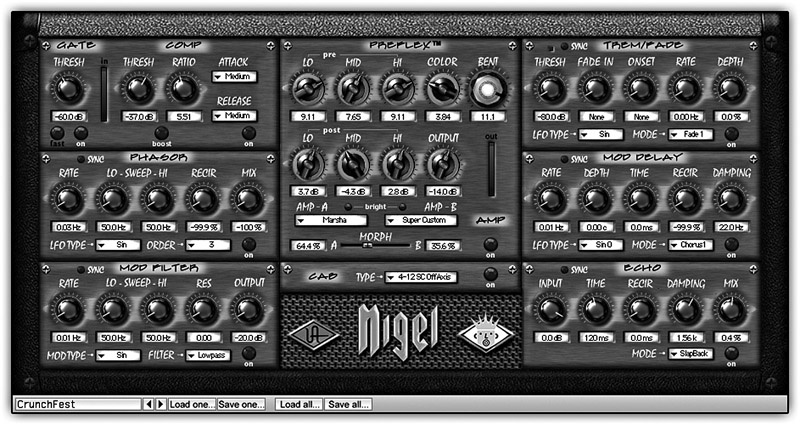
Figure 25.4 The Universal Audio Nigel. The center blocks on this plugin are the amp simulator where different amps and cabinets can be chosen. The side blocks provide additional effects such as tremolo and delay.

Dedicated units or plugins

As distortion becomes more popular, more dedicated units and even more plugins are appearing in the market. The Culture Vulture by Thermionic Culture is one respected hardware unit. The Soundtoys Decapitator, shown in Figure 25.5, is an analog saturation modeler plugin that can produce a variety of distortion options.

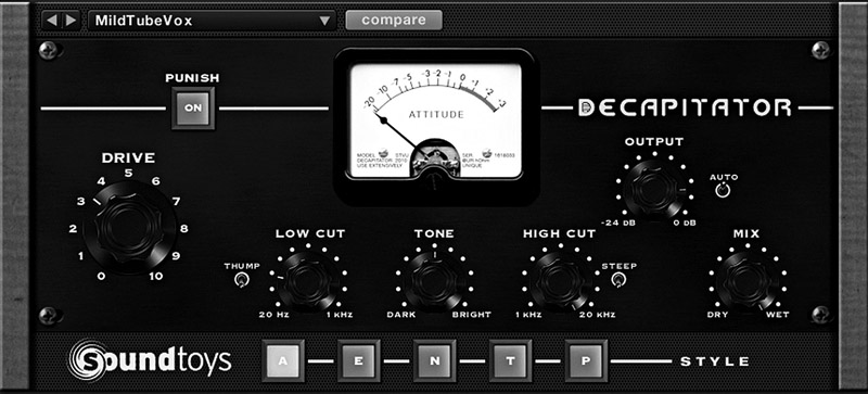
Figure 25.5 Soundtoys Decapitator plugin.