CHAPTER 7
Large Wire Loop Antennas
Loop antennas are characterized as small or large depending on the dimensions of the loop relative to the wavelength of the operating frequency. These two types of loops have different characteristics, work according to different principles, and serve different purposes. Small loops are those in which the current flowing in the wire has approximately the same phase and amplitude at every point in the loop (which fact implies a very short wire length, i.e., less than about 0.2λ). Such loops respond to the magnetic field component of the electromagnetic radio wave. A large loop antenna has a wire length greater than 0.2λ, with most being λ/2, 1λ, or 2λ. The current in a large loop varies along the length of the wire in a manner similar to other wire antennas whose length is comparable to λ/2. In particular, the direction of current flow reverses in each λ/2 section— a fact that is especially useful in the simplified analyses of loops we will use in the following sections.
λ/2 Large Loops
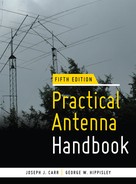
The radiation pattern of a large wire loop antenna is strongly dependent on its size. Figure 7.1 shows a half-wavelength loop (i.e., one in which each of the four sides is λ/8 long). Assuming S1 is in its closed position, the real part of the feedpoint (X1 – X2) impedance is on the order of 3 kΩ because it occurs at a voltage maximum. Unfortunately, the imaginary, or reactive, part of the impedance is closer to 20,000 Ω! This is an antenna that few antenna couplers can match, and one that has little to recommend it compared to a bent dipole in the same physical configuration with a 6-in insulator inserted in the midpoint of the wire segment opposite the feedpoint (corresponding to S1 being open).
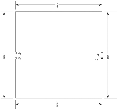
FIGURE 7.1 Half-wave square loop antenna.
The fundamental difficulty with the λ/2 loop is that the two ends of the wire appearing at the terminals of S1, each λ/4 from the feedpoint, carry high voltages that are out of phase with each other in normal operation of a half-wave dipole. Tying the ends together (by closing S1) forces the wire into an “unnatural” mode, resulting in abnormally high resistive and reactive components of feedpoint impedance.
Nonetheless, a simple trick can “tame” the difficult input impedance of the λ/2 loop. In Fig. 7.2, an inductor (L1 or L2) is inserted into the circuit at the midpoint of each wire segment adjacent to the driven segment. These inductors should have an inductive reactance XL of about 370 Ω at the center of the chosen operating band. The inductance of each coil is

FIGURE 7.2 Inductive loading improves λ/2 loop.
![]()
![]()
Example 7.1 Find the inductance for each coil in a loaded half-wavelength closed-loop antenna that must operate in a band centered on 10.125 MHz.
Solution Use Eq. (7.1).
(Note: 10.125 MHz = 10,125,000 Hz.)
![]()
The coils add lumped circuit inductive loading to the loop, giving it a greater effective length in a small space. The currents flowing in the antenna can be quite high, so, when making the coils, be sure to use a size that is sufficient for the power and current levels anticipated. The 2- to 3-in-diameter B&W Air-Dux style coils are sufficient for most amateur radio use. Smaller coils are available on the market, but their use should be limited to low-power situations.
1λ Large Loops
If space constraints are not forcing you to a λ/2 loop, then a 1λ loop might be just the ticket. Such a loop has many desirable features, including a manageable feedpoint impedance, more gain than a dipole in favored directions, and ease of analysis.
The simplest way to analyze the 1λ loop of Fig. 7.3 is to treat it as two horizontal half-wave “bent” dipoles whose outer halves are bent toward each other and connected together electrically. As we have seen in an earlier chapter, the center half of a λ/2 dipole is responsible for most of the radiated field strength; the ends establish resonance, minimize feedpoint reactance, and help raise the input or feedpoint impedance to a reasonable value. Thus, bending the outer halves of the dipoles 90 degrees has limited effect on the operation of the elements.

FIGURE 7.3 One-wavelength square loop (single-element quad).
Only one of the two dipoles is fed directly from the transmission line, and a short circuit is placed across the feedpoint of the other. Remember that current reverses direction in adjacent half-wave sections of a collinear array of dipoles. Thus, after an even number of half-wave segments, the drive current naturally wants to be in phase with the current coming around the full periphery of the loop. At the resonant operating frequency, the current goes to zero at what would be each end of the driven dipole and then reverses direction in the second dipole. This results in the currents in the horizontal sections of the two dipoles being in phase spatially—that is, they both point in the same direction (left or right in Fig. 7.3) at all times. In free space the 1λ loop is a two-element driven array, whereby the λ/2 section opposite the dipole connected to the feed-line is driven at its high-impedance ends, rather than at its center, from voltages set up by the fed dipole.
The 1λ loop of Fig. 7.3 produces a bidirectional gain of about +2 dB over a dipole in directions perpendicular to the plane of the loop—that is, into and out of the page. The elevation pattern formed by this loop is somewhat “squashed” because the top and bottom horizontal sections are in quadrature phasing straight up and down.
The loop of Figure 7.4 also contains one wavelength of wire, but the square has been put into a diamond orientation so that only one tall support is needed. In effect, we have replaced two bent dipoles with two inverted-vees facing each other, one above the other. Note that the connection to the feedline is no longer in the center of a leg but at a vertex joining two legs. Broadside to the loop (in and out of the page), the horizontal components of their radiation are in phase, but since the effective spacing of the two antennas is somewhat less than λ/2, they interact a bit differently from the square loop of Fig. 7.3, and the net gain compared to a single inverted-vee is compromised a bit. The vertically polarized component of radiation cancels out completely broadside to the loop and creates a weak cloverleaf in the plane of the loop (to the left and right on the page).

FIGURE 7.4 Bottom-fed diamond loop.
Broadside patterns of both the square and diamond loops look quite good in free space, showing 2- to 3-dB gain over a single dipole or inverted-vee, respectively. However, the presence of real ground beneath them compromises their array gain, especially on the lower HF bands, where few users will be able to raise the bottom of the loop much higher than λ/8 above ground, and array gains of 1 to 2 dB are more likely.
Delta Loop
The delta loop antenna, like the Greek uppercase letter “delta” (Δ) from which it draws its name, is triangular (Fig. 7.5). Although delta loops for VHF frequencies are often oriented point-down (as shown in the figure) to put the horizontally polarized radiating portion of the loop as high as possible, HF delta loops are far more often erected point-up so as to require only one high support. The wire required to form a delta loop is a full wavelength, with elements approximately 2 percent longer than the natural wavelength (like the quad). The actual length will be a function of the proximity and nature of the underlying ground, so some experimentation is necessary. For the isosceles triangle of Fig. 7.5, the approximate preadjustment lengths of the sides are found from:
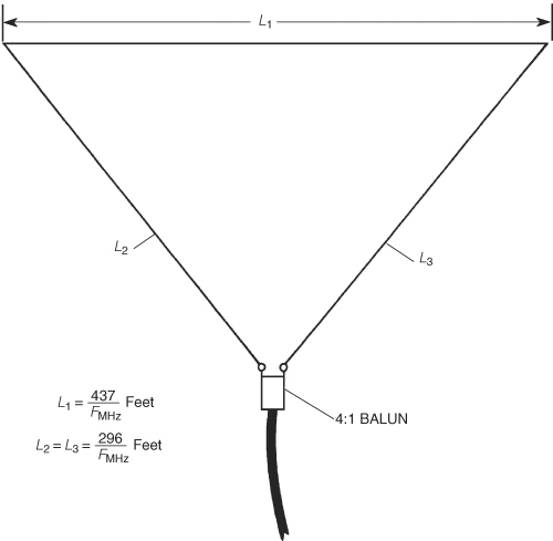
FIGURE 7.5 Delta loop antenna.
![]()
![]()
There is no reason, however, why your delta loop can’t be an equilateral triangle, in which case the starting point for each side is
![]()
Delta loops for 14 Mhz and above can be constructed from either copper wire or aluminum tubing, and are usually mounted on rotatable masts. Delta loops for 7 MHz and below are too large to be easily rotated, but fixed wire versions are popular with many amateurs.
The sharpness of the included angles on the delta loop is not particularly desirable and results in the antenna having less broadside gain than the square (quad) loop, but the triangular shape allows it to be suspended from a single high support. In all cases, maximum gain is in the two directions perpendicular to the plane of the loop.
The overall length of wire needed to build any of the preceding three 1λ loop antennas is
The polarization of the loop antennas fed as shown in Figs. 7.3 through 7.5 is horizontal because of the location of the feedpoint. That is because the highest-current sections of a 1λ loop are the two λ/8 sections that straddle the feedpoint, and the corresponding continuous λ/4 section halfway around the loop from the feedline. But there is nothing magic about that particular feedpoint location. On the square loop, moving the feedpoint to the middle of either vertical side will change the polarization to vertical. Similarly, on the diamond loop, vertical polarization is realized by moving the feedpoint to either of the two side vertices. On the delta loop, placing the feedpoint at either of the two other vertices produces a diagonal polarization that offers approximately equal vertical and horizontal polarization components, but vertical polarization is easily attained by moving the feedpoint one-fourth of the way up (or down, as the case may be) either side.
The feedpoint impedance of a 1λ loop is the vector combination of three components:
• Baseline feedpoint impedance of a simple λ/2 “bent” dipole or inverted-vee in free space
• Effect of radiated fields from the second λ/2 section on the fed section
• Ground reflection effects, if too close to ground to use free-space assumptions
The resulting input impedance for the array is around 110 Ω for any reasonable height above ground, so it provides a slight mismatch to 75-Ω coax and a 2:1 mismatch to 52-Ω coax. A very good matching to 52-Ω coax can be produced using the scheme of Fig. 7.6. Here, a quarter-wavelength coaxial cable matching section (see Chap. 4) is made of 75-Ω coaxial cable. The length of this cable should be

FIGURE 7.6 Quarter-wavelength coaxial matching section.
![]()

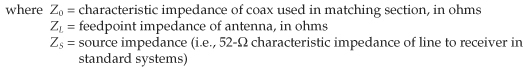
The impedance Z0 of the cable used for the matching section should be
![]()
When Eq. (7.4) is applied to a system having Zs = 52 Ω and ZL = 110 Ω:
![]()
This is a very good application of 75-Ω coaxial cable or CATV hardline.
Half-Delta Sloper (HDS)
The half-delta sloper (HDS) antenna (Fig. 7.7) is similar to the full delta loop, except that (like the quarter-wavelength vertical) half of the antenna is in the form of an “image” in the ground. Gains of 1.5 to 2 dB are achievable. The HDS antenna consists of two elements: a λ/3-wavelength sloping wire and a λ/6 vertical wire on an insulated mast (or a λ/6 metal mast). Because the ground currents are very important, much like the vertical antenna, either an extensive radial system at both ends is needed or a base ground return wire must be provided.

FIGURE 7.7 Half-delta loop (HDS) antenna.
The HDS will work on its design frequency, plus harmonics of the design frequency. For a fundamental frequency of 5 MHz, a vertical segment of 33 ft and a sloping section of 66 ft are needed. The approximate lengths for any frequency are found from
![]()
![]()
The HDS is fed at one corner, close to the ground. If only the fundamental frequency is desired, then you can feed it with 52-Ω coaxial cable. But at harmonics, the feedpoint impedance changes to as high as 1000 Ω. If harmonic operation is intended, then an antenna tuning unit (ATU) is needed at point A to match these impedances.
As with the delta loop, the “sharp” interior angle (i.e., <90 degrees) of the HDS is not ideal because components of the radiated fields from the different sections of the antenna will cancel in directions where other components are reinforcing.
2λ Bisquare Loop Antenna
When the size of the basic large loop is again doubled—this time to 2λ—loop analysis and patterns are no longer quite so clean and simple. As a general guideline, loops larger than 1λ have most gain in the main lobe (relative to a simple dipole) and “reasonable” feedpoint impedances only when the number and arrangement of λ/2 sections are such that the fields from multiple sections consistently reinforce each other in a few specific directions. One way to ensure this is to make sure the physical configuration of the loop results in currents on opposing sides of the loop being in phase with each other. Unfortunately, this becomes much more complicated for 2λ loops.
As an example, let’s return to the 1λ loop of Fig. 7.3. When fed at the center of the bottom horizontal λ/4 element, the horizontally polarized radiation of the top element reinforces that of the bottom element, and the primary gain is broadside to the plane of the loop, and horizontally polarized. Radiation from the upper half of each side element is canceled by out-of-phase radiation from the bottom half. So the predominant mode of operation for this antenna with the feedpoint located as shown is as a two-element horizontally polarized array.
If we now increase the length of each side to λ/2, we can consider this larger loop as comprised of four λ/2 dipoles, one on each side of the square, connected end to end and fed, as before, at the center of the bottom element. Noting that the current reverses in adjacent dipoles, we see that the current in the top element is now exactly out of phase spatially with the current in the bottom element. The same situation is true for the vertical currents in the two side elements. Because the top and bottom are λ/2 apart, as are the two sides, maximum horizontally polarized radiation is straight up and down (a cloud burner, in other words) and maximum vertically polarized radiation is to the left and right on the page. Thus, this loop antenna radiates best as a vertically polarized two-element array in the plane of the loop! Of course, in free space there is no such thing as “vertical” or “horizontal” and it doesn’t matter which side of the loop is fed—no matter what, it radiates end fire, not broadside. Unfortunately, the peak gain of the main vertically polarized lobe is only about 0.6 dB greater than for a single λ/2 vertical dipole. In the presence of a nearby ground, some small horizontally polarized lobes appear, but over any kind of real ground up to a height of 1.25λ for the top wire, the antenna does best as an end-fire vertically polarized array. If its overall length is adjusted for minimum reactance at the feedpoint, a 4:1 balun will make it a decent match to either 52-Ω or 75-Ω transmission line.
The 2λ bisquare antenna, shown in Fig. 7.8, is built like the diamond loop shown earlier (i.e., it is a large square loop fed at a vertex located at the bottom of the assembly) except that each side is now λ/2 in length. If the reactance is canceled out through slight shortening or lengthening of the total loop, the feedpoint impedance is a good match for either 52-Ω or 75-Ω cable directly. The difference in feedpoint impedances between the 2λ diamond loop and the 2λ quad loop is a direct result of changing the location of the feedpoint from the midpoint of a side to the corner between two sides.
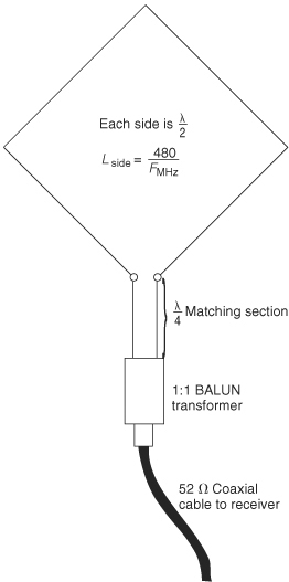
FIGURE 7.8 Bisquare 2λ square loop antenna.
When operated at its design frequency and fed as shown in Fig. 7.8, the bisquare antenna offers maximum horizontally polarized radiation in free space at a 45-degree elevation angle broadside to the plane of the antenna (42 degrees when the feedpoint is λ/4 above ground). The peaks of the vertically polarized radiation pattern are as before—that is, in the plane of the wire (to the left and right on the page), but the gain is 2 dB or so less than that of a single vertical λ/2 dipole, thus proving that “more” is not always “better”!
In general, there is little to recommend the added mechanical complexity of a 2λ loop unless the phase relationship between opposing sections is “corrected” with the use of phasing lines or inductors.
Near-Vertical Incidence Skywave (NVIS) Antenna
The preceding descriptions of large loop operation in the presence of ground are based on hanging each loop from one or two high supports. However, these loop antennas can instead be suspended so that the plane of the loop of wire is parallel to the ground beneath it. When that is done, at practical heights above ground these loops will send most of their radiation straight up in the air, since the innate array pattern of the 1λ loops generates maximum radiation at right angles to the plane of the loop.
Given the high-angle horizontal polarization of the bisquare loop, which favors short-haul communications links, comparable results can be obtained by laying the same amount of wire “on its side”, supported at a more practical height. A 2λ loop of wire arranged in a diamond of uniform height λ/8 or more can provide nearly the same gain as the bisquare, albeit in a more omnidirectional pattern. Actually, the pattern of the 2λ NVIS antenna consists of two separate four-lobed cloverleafs: one with horizontally polarized lobes at right angles to the four wires, and the other with vertically polarized lobes midway in between.