CHAPTER 22
Radio Astronomy Antennas
For centuries astronomers have scanned the heavens with optical telescopes. But today, astronomers have many more tools in their bag, and one of them is radio astronomy. The field of radio astronomy emerged in the 1930s and 1940s through the work of Grote Reber and Carl Jansky. Even during World War II, progress was made as many tens of thousands of operators were listening to frequencies from “dc to daylight” (well, actually, the low end of the microwave bands). British radar operators noted during the Battle of Britain that the distance at which they could detect German aircraft dropped when the Milky Way was above the horizon.
Although there is a lot of amateur radio astronomy being done, most of it requires microwave equipment with low-noise front ends and is beyond the scope of this book. For example, most deep space (beyond our solar system) radio sources will require the use of high-gain configurations—such as long baseline arrays—that are far beyond any one individual’s ability to implement. However, there are several things that almost anyone can do as an introduction to this “hobby within a hobby”.
Radio astronomy antennas can assume nearly all forms. It is common to see Yagis, ring Yagis, cubical quads, and other antennas for lower-frequency use (18 to 1200 MHz). Microwave gain antennas, such as parabolic reflectors, can be used for higher frequencies. Indeed, many amateur radio astronomers employ TV receive-only (TVRO) satellite dish antennas for astronomy work. In this chapter we limit our coverage to some antennas that are not discussed in other chapters—at least, not in this present context.
General Considerations
The strongest extraterrestrial radio sources we can typically detect are from our own sun. These emissions are very broadband and so our receivers typically detect only a small portion of the total radiated spectrum at any one time. When we listen on a receiver, using conventional heterodyne reception feeding a loudspeaker, what we hear is noise that varies in amplitude—sometimes slowly, sometimes in bursts.
As a rule, we are restricted to monitoring the sun and other astronomical bodies at frequencies higher than those blocked by earth’s ionosphere. The low end of the useable frequency range varies with the sunspot cycle, time of day, etc., but frequencies above 18 MHz, as mentioned, should work virtually all the time. Many radio astronomers, both amateur and professional, concentrate on the region around 20.1 MHz, but the author has heard the sun on 28 MHz many times with a simple three-element Yagi. Of course, if these bands are open for HF skip propagation, or if many local ground-wave signals are present, other frequencies may contain fewer interfering terrestrial signals.
So what do you need to chase DX throughout our solar system? All it takes is a receiver that works well over the range from 18 to 30 MHz—most modern communications receivers are fine for the purpose—and a relatively simple antenna tuned to some portion of that frequency span. Any automatic gain control (AGC) or automatic volume control (AVC) should be turned off, the audio volume control set to a comfortable level, and the RF gain control advanced at least to the point where external noise overrides the internal noise of the receiver. Set your receiver to the single sideband (SSB) mode and select the widest filter bandwidth(s) available.
Today, of course, inexpensive PCs and software applications allow us to “listen” with our eyes, as well. Spectrograms and other displays of the received signals allow us to see and print out evidence of these astronomical noise bursts. A simple Internet search should return a host of how-to articles, blogs, and discussion groups.
Listening to “Ol’ Sol”
Even a dipole has directivity, so it’s helpful to orient even the simplest of antennas with the peak response of its pattern in the direction of the source. Since the sun’s path for many of us covers such a broad range of both azimuth and elevation angles, it’s probably smartest to zero in on its location for those hours of the day that we’re most apt to be able to listen for it.
Of course, for dipoles at 18 MHz and above, rotating them is a relatively simple task, whether done manually or with an antenna rotator.
At some point, you may wish to add greater gain and directivity to improve your ability to pull extraterrestrial signals out of your background noise environment, especially if you are in an urban neighborhood. Even then, rotating a two- or three-element Yagi at 20 MHz and higher is not an insurmountable task. Best yet, antenna height is not a factor—especially if you stick to listening periods when the sun is well above the horizon.
Signals from Jupiter
Second only to the sun, Jupiter is a strong radio source. It produces noiselike signals from VLF to 40 MHz, with peaks between 18 and 24 MHz. One theory attributes the radio signals to massive storms on the largest planet’s surface, apparently triggered by the transit of the Jovian moons through the planet’s magnetic field. The signals are plainly audible on the upper HF bands any time Jupiter is above the horizon, day or night. However, in order to eliminate the possibility of both local and terrestrial skip signals from interfering, Jupiter DXers prefer to listen only when the maximum useable frequency (MUF) drops significantly below 18 MHz—typically the darkness hours. In preparation, listen to the amateur 17- or 15-m bands; if you hear no skip-distance activity, then it’s a good bet that the MUF has dropped enough to make listening worthwhile. Even during the day, however, it is possible to hear Jovian signals, but differentiating them from other signals and solar noise can be difficult.
Jupiter emits two distinctly different types of radio noises. Listening in SSB mode, one form can be heard as “swooshing” noises that rise and fall in amplitude over a relatively long interval. The second type of noise from the planet is heard as a more rapid-fire “popping” sound.
Unlike the sun, Jupiter does not often rise high in our sky. Its transit, as viewed at midlatitudes in the northern hemisphere, is typically close to the horizon—rising in the southeast and setting in the southwest. In that respect, Jupiter is an excellent target for a typical HF Yagi or cubical quad whose height has been optimized for low elevation angles. Also, Jupiter is visible (and audible) at times totally unrelated to our day and night periods. As a result, there may be periods when Jupiter’s emissions may be difficult to hear because the sun is also “in your face”. Search the Internet for detailed calendars of Jupiter’s transits.
For monitoring Jupiter, a good beginning antenna can be a simple dipole cut for the middle of the 18- to 24-MHz band, which happens to coincide with the 15-m amateur radio band. The antenna should be installed in the normal manner for any dipole, except that if it is fixed in one position the wire should run east-west in order to maximize pickup from this southerly rising planet.
Figure 22.1 shows a broadband dipole that covers the entire frequency span of interest (18 to 24 MHz) by paralleling three different dipoles: one cut for 18 MHz, one cut for 21 MHz, and one cut for 24 MHz. The dimensions are

FIGURE 22.1 Wideband HF dipole for Jupiter reception.

As discussed in the chapter on multiband wires (Chap. 8), there are several approaches to making this type of antenna. One is to use three-conductor wire and cut the wires to the lengths indicated here. Another is to use a homemade spacer to spread the wires apart.
Ring Antenna
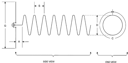
Another popular Jovian radio antenna is the ring radiator, two versions of which are shown in Fig. 22.2. This antenna is made of a 5-ft-diameter loop of ½-in-diameter soft-drawn copper plumbing pipe found in any local hardware or plumbing supply store. The single-ended version is shown in Fig. 22.2A. In this form the far end of the loop is unterminated (i.e., open-circuited). The center conductor of the coaxial cable feedline is connected to the near end of the ring radiator, while the coax shield is connected to the chicken wire ground plane. The balanced version (Fig. 22.2B) has an RF transformer (T1) at the feedpoint.

FIGURE 22.2A Ring radiator: single-ended.

FIGURE 22.2B Ring radiator: balanced.
The ring radiator antenna should have a bandpass-filtered preamplifier—needed because of the antenna’s low output levels. The preamp should be mounted as close as possible to the antenna. The intent is to minimize the likelihood of strong terrestrial signals in the adjacent bands desensing the preamp or receiver. Even a 5W CB transmitter a few blocks away can drive the preamplifier into saturation, so it’s wise to eliminate the undesired signals before they get into the preamplifier. In the case of the single-ended amplifier, a single-ended preamplifier is used. But for the balanced version (Fig. 22.2B) a differential preamplifier is appropriate.
Either version of the loop or ring is mounted about 7 or 8 in above a ground plane made of chicken wire, metal window screen, copper sheeting, or copper foil. (Copper sheeting or foil is best but costs a lot of money and turns ugly green after a couple weeks in the elements.) If you use screening, make sure that it is metallic. Some window and porch screening material is made of synthetic materials that are insulators.
Figure 22.3A is a mechanical side view of the ring radiator antenna, while Fig. 22.3B is a top view. The antenna is mounted above the screen with insulators. These can be made of wood, plastic, or any other insulating material. The frame holding the ground-plane screen (Fig. 22.3B) can be made from 1- × 2-in lumber. Note that the frame is strengthened by interior crosspieces that also support the antenna. The larger outer perimeter is needed because the screen ground plane should extend beyond the diameter of the radiator element by at least 10 to 15 percent of that dimension.
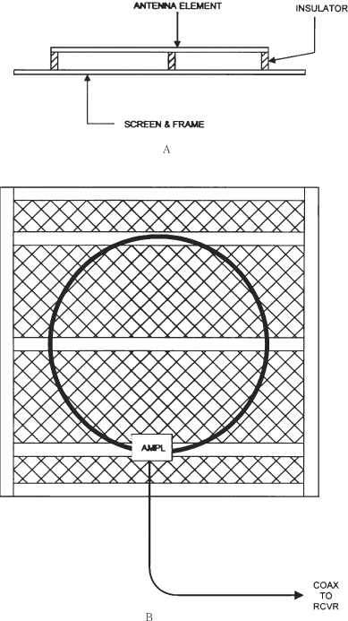
FIGURE 22.3 Ring radiator mounted over a ground screen.
DDRR
The directional discontinuity ring radiator (DDRR) antenna is shown in Fig. 22.4A, while a side view showing the mounting scheme is shown in Fig. 22.4B. The DDRR is typically mounted about 1 ft off the ground (H = 12 in). It consists of two sections, one vertical and one horizontal. The short vertical section has a length equal to the height H of the antenna above the ground, and the lower end of the vertical segment is grounded.

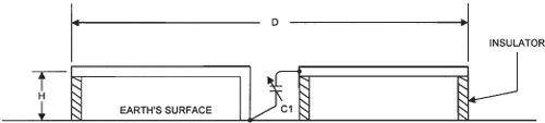
FIGURE 22.4B DDRR antenna: side view.
The horizontal section is an open-circuited loop of diameter D, which varies with frequency.
The optimum conductor diameter E for the DDRR is at least 0.5 in at 28 MHz, increasing to 4 in at 4 MHz. Thus, for monitoring Jupiter, a diameter of 1 in or slightly less is appropriate.
Because of the loop, some people call this the hula hoop antenna. One author recommends using a 2-in automobile exhaust pipe bent into the correct shape by a cooperative automobile muffler mechanic. The far end of the loop is connected to ground through a small-value tuning capacitor C1. The actual value of C1, which is used to resonate the antenna at a particular operating frequency, is found experimentally.
The feedline of the DDRR antenna is coaxial cable; its shield is grounded at the bottom end of the vertical section. The center conductor is connected to the ring radiator a distance F from the vertical section in a circular variant of the autotransformer or gamma match. The length F is determined by the impedance that must be matched. The radiation resistance is approximated by
![]()

H and λ must be in the same units.
The approximate values for the various dimensions of the DDRR are given as follows in general terms, with examples in Table 22.1:
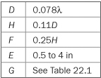

TABLE 22.1 Examples of Dimensions for DDRR
The construction details of the DDRR are so similar to those of the ring radiator that the same diagram can be used (see Fig. 22.3 again).
The normal attitude of the DDRR for communications is horizontal. However, for maximum signal when monitoring Jupiter, the entire antenna assembly, including the ground-plane screen, can be tilted to track Jupiter’s position in the sky.
Helical Antennas
The helical antenna (Fig. 22.5) provides moderately wide bandwidth and circular polarization. Thanks to the latter, some find the helical antenna particularly well suited to radio astronomy reception. The antenna (of diameter D) will have a circumference C of 0.75λ to 1.3λ. The pitch of the helix (S) is the axial length of a single turn, while the overall length L = NS (where N is the number of turns). The ratio S/C should be 0.22λ to 0.28λ. At least three turns are needed to produce axial-mode main lobe maxima.
The diameter or edge of the ground plane G should be on the order of 0.8λ to 1.1λ if the conducting surface is circular or square, respectively. The offset between the ground plane and the first turn of the helix is 0.12λ.
The approximate gain of the helical antenna is found from
![]()
The pitch angle ϕ and turn length γ for the helical antenna are given by
![]()
and
![]()
The beamwidth of the helical antenna is
![]()

K is 52 for the –3-dB beamwidth and 115 for the beamwidth to the first null in the pattern.
The short section between the helix and the ground plane is terminated in a coaxial connector, allowing the antenna to be fed from the rear of the ground plane. The feedpoint impedance is approximately 140 Ω.
Multiple Helical Antennas
Stacking helical antennas allows a radiation pattern that is much cleaner than the normal one-antenna radiation pattern. It also provides a good way to obtain high gain with only a few turns in each helix. If two helixes are stacked, then the gain will be the same as for an antenna that is twice the length of each element, while for four stacked antennas the gain is the same as for a single antenna four times as long. Figure 22.6 shows a side view of the stacked helixes.
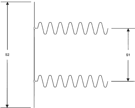
FIGURE 22.6 Dual/quad helical antenna.
The feed system for stacked helixes is more complicated than for a single helix. Figure 22.7A shows an end view of a set of four stacked helical antennas. Tapered lines (TL) are used to carry signal from each element and the coaxial connector (B). In this case, the coaxial connector is a feed-through barrel or back-to-back SO-239 device at the center of the ground plane (B). A side view of the tapered line system is shown in Fig. 22.7B. The length of the tapered lines is 1.06λ, while the center-to-center spacing between the helical elements is 1.5λ. The length of each side of the ground plane is 2.5λ. In the case of Fig. 22.7, the antenna is fed from the front of the ground plane.

FIGURE 22.7 Front view of quad helical antenna.
Interferometer Antennas
The resolution of an antenna is a function of its dimensions relative to the wavelength λ of the received signal. Better resolution can be achieved by increasing the size of the antenna, but that is not always the best solution and beyond a certain point is totally impractical. Figure 22.8 shows a summation interferometer array. Two antennas, each with aperture a, are spaced S wavelengths apart. The radiation pattern is a fringe pattern (Fig. 22.9), consisting of a series of maxima and minima. The resolution angle ϕ to the first null is
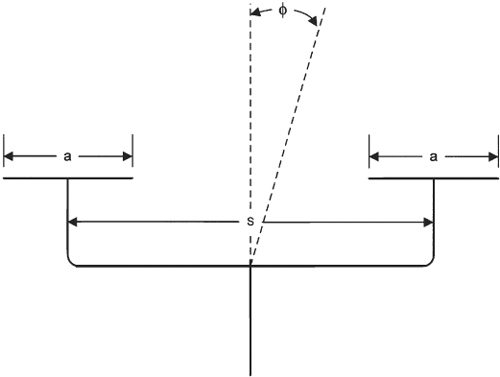
FIGURE 22.8 Interferometer array.

FIGURE 22.9 Interferometer pattern.
![]()
The interferometer can be improved by adding antennas to the array. Professional radio astronomers use very long or wide baseline antennas. With modern communications it is possible to link radio telescopes on different continents to make the widest or longest possible terrestrial baseline.