CHAPTER 11
Vertical Arrays
Despite its longevity, the vertical antenna is either praised or cursed by its users, depending upon their experiences with it. At HF in particular, “DXability” is often the criterion for judging the antenna’s performance. As amateurs and others have come to appreciate the importance of a good RF ground system to the vertical’s performance, in recent years the vertical has come into its own on the 1.8- and 3.5-MHz bands because it provides superior low-angle radiation compared to the low dipoles that are the only alternative for most users.
But a vertical antenna is omnidirectional in its azimuthal (compass rose) coverage; that is, it transmits and it “hears” equally well in all directions. Thus, a single vertical exhibits two weaknesses:
• It puts far more RF energy out in directions that are of no use (at that particular moment, at least) than it does in the desired direction.
• It does not have any way of eliminating noise coming from all 360 degrees around the compass when trying to receive a weak signal from a specific heading.
With respect to the first point, there are only three things the user with a single vertical can do to improve his/her signal at a specific faraway receiving location:
• Increase the transmitter power to the antenna.
• Improve the antenna efficiency by reducing resistive losses, especially by making sure an adequate system of radials is installed at the base of the antenna.
• Increase the electrical length of the vertical radiator (up to a maximum of 5 λ/8). This causes the low-angle field strength for a given transmitter power to increase because high-angle radiation is being reduced as the vertical is lengthened.
With respect to the second point, we note:
• Atmospheric band noise arrives from compass headings where the band is “open”. That is, if it’s shortly after sunset at the site of the vertical antenna, atmospheric noise on the MF and lower HF bands is likely coming only from points east of the antenna, where darkness and ionospheric propagation are prevalent. To the west, daylight absorption in the lower layers of the ionosphere substantially reduces the noise levels at the vertical. This is true of the noise (“QRN” in the long-established radio shorthand known as Q-signals) from distant thunderstorms.
• Nearby thunderstorms, on the other hand, can be heard equally well regardless of their location relative to the vertical, since the propagation mode is likely direct line of sight from clouds in the region to the antenna.
• Man-made noise (“QRM”) is usually (but not always) nearby and unaffected by ionospheric propagation conditions. Today most man-made QRM originates in the high-speed microprocessors and digital circuits that infest all the appliances and electronics gear in our homes and offices or those of our neighbors. In general, we have little or no control over the direction of these sources from our vertical, so we can assume that their compass headings are likely to be randomly distributed.
Directivity and Phasing
We can improve our ability to hear and to be heard on any frequency—but especially on the MF and lower HF bands—where we are using a vertical antenna by operating two or more in an array. As we saw in Chap. 5, arrays can provide increased field strength in some directions at the expense of strength in other directions. This holds for both transmitting and receiving, so an array of vertical antennas can help overcome all but one of the limitations itemized in the preceding bullet list. (An array will not help us reduce atmospheric noise or QRM coming from the same direction as a weak signal we are trying to copy.)
Most AM broadcast stations have used arrays of vertical antennas for decades. Consequently, the best radio engineers of the past century have collectively designed and evaluated far more combinations of verticals than any one author could do on his or her own in a lifetime, and there is much to be learned and borrowed from the AM broadcast band favorites. Many standard patterns for two-, three-, four-, and five-vertical arrays dating from before World War II exist in the literature. Most of the more complicated ones are irrelevant to anything other than the AM broadcast band, but the simpler combinations have many virtues useful to amateurs and others.
Of course, amateurs and shortwave or broadcast band listeners usually have a requirement that AM broadcast stations do not: Most arrays must be designed so they can be switched or steered to more than one compass heading.
To do the subject of vertical arrays full justice would require a separate book at least as big as this one. So this chapter will serve primarily as an overview of some simple but effective arrays that can be formed with the proper placement and feed systems.
In general, an array of verticals involves two or more antennas in close proximity, each fed at a specified phase angle and amplitude relative to a common reference in order to produce the desired radiation pattern. Often the common reference is simply the RF applied to one of the antennas in the array that has been selected to serve as the reference point.
Two-Element Array
Figure 11.1 shows the possible patterns for a pair of vertical antennas spaced a half-wavelength (180 degrees) apart and fed in phase or (180 degrees) out of phase. Although other phasing relationships between the drive currents to the two antennas are possible, we’ll stick with these because of the simplicity of the networks required to feed them.
When the two verticals (A and B) are fed in phase with equal currents, the radiation pattern of Fig. 11.1A (idealized here) results. It is a bidirectional figure eight that is maximum broadside to a line drawn between the two antennas. If there are no nearby obstructions and the ground around the two verticals is reasonably flat and featureless, and if the drive currents to the two antennas are well matched in both amplitude and phase, a deep null is formed along the axis of the array—i.e., along the line drawn between the elements A and B.
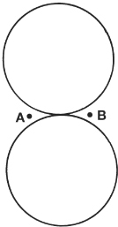
FIGURE 11.1A Pattern of two radiators fed in phase, spaced a half-wavelength apart.
If the phase of the drive current to one of the elements is shifted by 180 degrees, the pattern rotates 90 degrees (a quarter of the way around the compass) and now exhibits directivity along the line of the centers (A-B), as depicted in Fig. 11.1B. This is often called an end-fire pattern or an end-fire array.
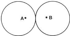
FIGURE 11.1B Pattern of two radiators fed out of phase, spaced a half-wavelength apart.
Note that the forward gains and the exact shapes of the broadside and end-fire patterns are seldom the same.
The simplest way to make sure the amplitudes of the feed currents to the two array elements are identical is to bring a common feedline from the transmitter to a point midway between the two elements and then feed each element from there. Figure 11.2A shows the feedline configuration for driving the array elements in phase; note, in particular, that lengths L1 and L2 must be the same, and ideally they should be cut from the same roll of coaxial cable or hardline so that their impedances and velocities of propagation are as closely matched as possible.
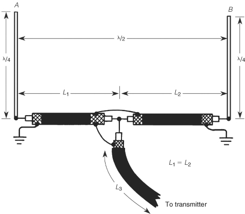
FIGURE 11.2A Feeding a phased array antenna in phase.
To switch the two-element array to its end-fire mode of Fig. 11.1B an extra 180-degree phase shift must be added to the drive signal delivered to one or the other (but not both) of the two elements. Although this phase shift can be provided with a discrete component LC network, a simple solution is to add an extra λ/2 section of the same cable in the line to one element. When doing so, it’s important to include the velocity factor (vF) of the cable in the calculation. vF is a decimal fraction on the order of 0.66 to 0.90, depending upon the specific transmission line used. Its effect is to cause a line that is electrically λ/2 to be much shorter than λ/2 physically. In particular:
Example 11.1 Assuming the use of standard RG-8U coaxial cable with a velocity factor of 0.67, a half-wavelength section of cable for 3.6 MHz is
![]()
If we are interested only in the end-fire pattern of Fig. 11.1B, we can feed the array as shown in Fig. 11.2B, where it is understood that the lengths shown for the segments of coaxial cable are electrical lengths, not physical lengths. If, instead, we wish to be able to switch back and forth easily between broadside and end-fed modes, we can use the circuit of Fig. 11.3. Here two convenient, but equal, lengths of coaxial cable (L1 and L2) are used to carry RF power to the antennas. One segment (L1) is fed directly from the transmitter’s coaxial cable (L3), while the other is fed from a phasing switch. The phasing switch is used to either bypass or insert a phase-shifting length of coaxial cable (L4).
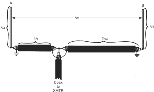
FIGURE 11.2B Minimum length feed for a phased array antenna.

FIGURE 11.3 Phase-shifting antenna circuit.
In principle this technique allows the selection of varying amounts of phase shift from 45 degrees to 270 degrees. However, at other than 0 degrees and 180 degrees, the currents no longer split equally between the two elements because the element feedpoint impedances are not the same. In general, for angles other than 0 degrees or 180 degrees, more complicated feed systems, including current-forcing techniques, are employed.
When unequal lengths of transmission line go to the elements of an array, unequal amplitudes are a likely by-product. The most noticeable effect for small differences, such as would occur when adding a λ/2 section of cable to implement the end-fire mode, will be to cause the nulls to fill in and lose some of their depth.
With the addition of a phasing transformer, a two-element vertical array can be remotely switched between broadside and end-fire modes while preserving balanced drive currents at the two elements. Figure 11.4 shows how a two-element array is fed through such a two-port phasing transformer. The phase-reversing switch S1 can, of course, consist of coaxial relays controlled from the transmitter end of the transmission line. The transformer itself is made from a 1:1 toroidal balun kit such as those available from Amidon Associates and others.
Wind the three coils in trifilar style, according to the kit instructions. The dots in Fig. 11.4A show the “sense” of the coils, and they are important for correct phasing; call one end the “dot end” and the other end the “plain end”—and mark them differently—to keep track of them. If the dot end of the first coil is connected to J3 (where the feedline from the transmitter or receiver attaches), connect the dot end of the second coil to the 0-degree output (J1, which goes to array element A). The third coil is connected to J2 through a DPDT low-loss RF relay or switch rated for the power levels involved. Although the transformer adds a small amount of loss, it is applied equally to both elements, so the amplitudes of their drive currents remain equal regardless of which mode the array is operated in.
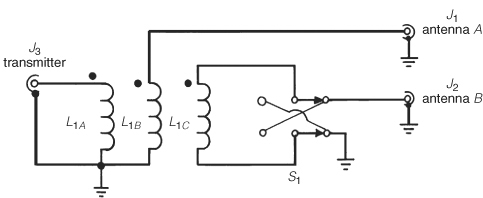
FIGURE 11.4A Phasing transformer circuit.
Be very sure, as shown in Fig. 11.4B, the coaxial cables to the individual elements are identical lengths from the point where they connect to J1 and J2 on the transformer housing to the base of either element.

FIGURE 11.4B Connection to antennas.
360-Degree Directional Array
The phased vertical antenna concept can be used to provide round-the-compass steering of the antenna pattern. Figure 11.5 shows how three λ/4 verticals (arranged in a triangle that is a half-wavelength on each side) can be used to provide unidirectional and bidirectional patterns through combinations of in-phase, out-of-phase, and grounded elements. For a specific pattern, any given element (A, B, or C) is grounded (“passive”), fed at 0-degree phase, or fed with 180-degree phase shift.
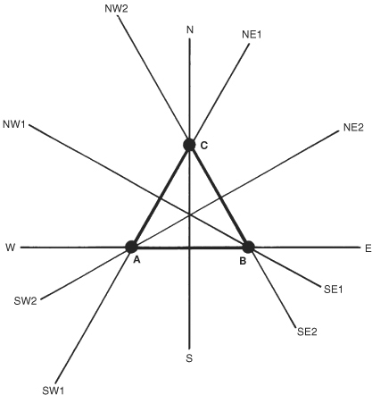
FIGURE 11.5 Three-element phased array.
Table 11.1 lists for each compass direction the drive to each of the three elements, the maximum forward gain of that configuration and the elevation angle at which it occurs, and a rough front-to-back (F/B) number. The figures in Table 11.1 are specifically for a three-element 80-m array with identical 66-ft verticals spaced 136 ft (λ/2) apart. The design frequency is 3.6 MHz. Each element has fifteen 65-ft radials at its base. Any time an element is labeled “Passive” in the table, it is unfed and directly grounded to the radial field beneath it.

TABLE 11.1 Pattern Gains for Three-Element Equilateral Array of Fig. 11.5.
In practice, at any specific location the triangular footprint of the three verticals can be rotated up to 60 degrees in either direction relative to the compass headings shown to orient the best patterns where they can be of most help. (Notice that each type of pattern repeats every 120 degrees.) Some of the patterns listed in the table have little to recommend them, but, as a general rule, most amateur DXers on the MF and HF bands find that breaking the 360-degree compass rose into six 60-degree directions is more than adequate.
If space is at a premium, or if multiband operation of an array of trap verticals is desired, the same equilateral triangle can be used with shorter spacings between the verticals. For years, Hy-Gain published an application note that detailed how to feed three of their 18-AVQ trap verticals spaced λ/8 apart at the lowest frequency (80 m) they covered. One of the difficulties with spacing other than λ/2 is that 180-degree phase shifts in drive current are no longer matched by the phase shift undergone by the radiated wave as it heads from one element to another; instead, spatial phase shifts of 45 degrees and 90 degrees are involved on 80 m and 40 m, respectively, and multiples of 360 degrees (i.e., in phase) on bands above 20 m. Nonetheless, directivity and gain are possible with such a system.
Four-Square Array
Another popular way to obtain directivity that can be switched to multiple compass headings is the four-square (or 4-square) array. In its original implementation, four λ/4 vertical monopoles are located at the corners of a square that is λ/4 on a side. Drive currents of equal amplitudes are applied to all four elements, but with three different phases. To develop maximum gain along a diagonal of the square, if the rear vertical on the diagonal is defined to have zero phase shift, the front vertical (i.e., the one in the direction of maximum gain) is –180 degrees and the two side verticals are both –90 degrees. Obviously, all aspects of the array’s performance can be identical every 90 degrees around the compass, simply by switching the phase of the drive current going to each specific vertical.
An amateur DXer in the northeastern United States would likely orient his or her 4-square so as to put the center of the four switchable pattern lobes at 60-, 150-, 240-, and 330-degree compass headings to favor Europe/North Africa, South America, Australia/New Zealand, and the Far East, respectively.
Other variations of the 4-square utilize somewhat different combinations of phase shifts and/or smaller spacings between elements. In most cases, 4-squares are constructed with ground-mounted monopoles and extensive radial fields, but today many employ elevated radial systems. If the user has the means to “force” drive currents of arbitrary phase and amplitude relationships to the four elements, there’s virtually no limit to the number of customized azimuth patterns that can be obtained.
Receive-Only Vertical Arrays
Much work has been done in the past few years on phased arrays for receiving at MF and the lower HF bands. In stark contrast to the challenges of weak signal reception at VHF and above, the abundance of atmospheric noise below, say, 10 MHz gives the system designer additional leeway in selecting techniques for digging weak signals out of the background noise. At these low frequencies, receive-only arrays can differ from their transmitting antenna counterparts in two important ways:
• Because receive-only arrays are not used for transmitting, antenna efficiency is of only secondary importance; as a result, array elements much shorter than λ/4 and having very low feedpoint impedances as well as inexpensive tubing and support requirements can be employed, and preamplifiers (if needed) added at the array.
• Because no transmitted RF energy is directly applied to the elements, there is no need for high-voltage or high-current components that are normally required for transmit applications.
Over the past decade or two, leading 160-m and 80-m DXers fortunate enough to have the necessary acreage have designed and built six-circle and eight-circle arrays for these bands. Typical of these arrays, which provide outstanding receive directivity and signal-to-noise ratio (SNR) on these notoriously weak-signal frequencies, is the eight-circle for 160 m designed by Tom Rauch, W8JI. In this design, the output signals from four of eight short vertical elements equispaced around the circumference of a circle are combined with appropriate relays and phasing lines to provide more than 7 dB gain in the desired direction, relative to a single such element. Because the circle of elements is eight-way symmetrical around the compass rose, the main lobe can be switched in 45-degree increments.
At any given switch position (i.e., compass heading), only four of the eight elements are active: Two adjacent elements on one side of the circle form an end-fire two-element array, as do two adjacent elements directly opposite, on the far side of the circle. These two end-fire arrays are then combined in a two-element broadside array, thus enjoying high forward gain and deep nulls to the rear, thanks to the principle of pattern multiplication. Both the eight-circle and the four-element combined end-fire/broadside array building block are described in detail by John Devoldere in his excellent book ON4UN’s Low-Band DXing, published by ARRL.
Although circle arrays for a given frequency range require less acreage than four bidirectional Beverage antennas, an absolute minimum for a 1.8-MHz eight-circle is about three acres, assuming ideally shaped property. Recently, John Kaufman, W1FV, has designed and published (through ARRL) a compact dual-band version of a nine-circle array requiring a very modest 140-ft-diameter footprint (corresponding to slightly more than a half-acre). The W1FV array consists of eight elements around the periphery of the circle, surrounding a single element at its center. It functions as a three-element in-line array that—just like the eight-circle—can be switched in 45-degree heading increments. The 160-m design acquits itself quite nicely on 80 m, as well, thus eliminating the need for the added costs (and acreage,) of a separate 80-m receiving array.
As we have said many times throughout this book, there is no “free lunch”. High-performance arrays of short receiving elements are precision designs, requiring close matching of signal amplitudes and differential phase shifts from element to element. Poor feedline installations and sloppy grounding techniques, among other things, can lead to common-mode signal pickup and other ills that will easily nullify the directivity and SNR improvements possible with these antennas.
Grounding
It goes without saying that no ground-mounted or ground-plane vertical will perform very well without an adequate ground system beneath it. This is especially true for arrays of verticals, as well. Each element of an array of vertical monopoles should have its own extensive ground system (the W1FV array is an exception to this), whether composed of sheets of copper flashing, two dozen or more radials each generally as long as the vertical is tall, or saltwater. If radials or other conductors are employed, they should not be allowed to overlap unless they are insulated or unless all points of possible contact have been soldered or mechanically joined. Intermittent or oxidized joints can raise the background noise level when receiving and result in the radiation of spurious out-of-band signals when transmitting. Refer to the grounding information in Chaps. 9 and 30 for a more extensive discussion of grounding techniques.